The Economic Case for a Pandemic Fund

Abstract

The rapid urban spread of Ebola virus in West Africa in 2014 and consequent breakdown of control measures led to a significant economic impact as well as the burden on public health and wellbeing. The US government appropriated $5.4 Billion for FY2015 and WHO proposed a $100 Million emergency fund largely to curtail the threat of future outbreaks. Using epidemiological analyses and economic modeling, we propose that the best use of these and similar funds would be to serve as global insurance against the continued threat of emerging infectious diseases. An effective strategy would involve the initial investment in strengthening mobile and adaptable capacity to deal with the threat and reality of disease emergence, coupled with repeated investment to maintain what is effectively a ‘national guard’ for pandemic prevention and response. This investment would create a capital stock that could also provide access to safe treatment during and between crises in developing countries, lowering risk to developed countries.

Introduction

The 2013–2015 West African Ebola virus disease outbreak (hereinafter termed “W. African Ebola outbreak”) lasted more than 1 year and was longer and larger (65 times the next largest historical outbreak) than any prior outbreak, with 27,678 reported cases in 10 countries and 11,276 reported deaths as of July 15, 2015 (World Health Organization 2015a, b; Table 1). Most previous outbreaks have been localized to a single country, and only 7 have caused more than 100 known cases prior to 2013, with the largest of these affecting 425 people (Centers for Disease Control and Prevention 2014; Table 1). The unprecedented scale of the 2013–2015 outbreak highlights a critical weakness in our global battle against the threat of pandemics—the lack of a well-funded, long-term strategy to pre-empt pandemic emergence. Pandemics originate from sporadic, but frequent emerging disease events that are caused largely by socioeconomic and environmental changes (Morse et al. 2012). As prior pandemics have occurred, societal response has included initiatives designed specifically to thwart their origin and spread, e.g., broadening of the International Health Regulations (IHR) following the SARS outbreak (Orellana 2005; Heymann et al. 2015). These initiatives are often coupled with surges of funding for basic and applied research to reduce future threats. However, these are often subject to waning public interest in the inter-pandemic intervals between perceived threats. For example, in the USA, the 2001 anthrax attacks led to a surge of funding to counter potential bioterrorism agents (‘select agents’) much of which supported strategies of value to other pandemic pathogens (Morens et al. 2004; Khan 2011). The emergence of H5N1 avian flu and H1N1 pandemic flu each led to funding for the development and purchase of medical countermeasures (vaccines and drugs) and for basic science and capacity building in countries of high prevalence (Collin et al. 2009; Walley and Davidson 2010). Following the largest ever Ebola outbreak in 2013–2015, the US President requested $6.18 billion and Congress allocated emergency funding of $5.4 Billion for control and prevention programs (The White House Office of the Press Secretary 2014; Mikulski 2015). The World Health Organization (WHO) announced a $100 million emergency fund to avoid impacts of future emerging diseases (Reuters 2015). Here we use epidemiological and economic analyses to examine whether this could be considered another step in a boom-bust cycle of pandemic threat and response, or the beginning of a new strategy to pre-empt the repeated emergence of pathogens with pandemic potential. We then examine how these funds could be spent to best reduce the opportunity for future global health emergencies of the same scale as the 2013–2015 West African Ebola outbreak.

Table 1.

Outbreak Data.

Outbreak	Initial region	Region area	Region population	Region density	Initial date	Initial cases	Initial deaths	Cases	Deaths
ebov1	Nzerekore, Faranah	148,555.0	5,933,479	39.9	2014-03-22	80	59	27,678	11,276
ebov2	Northern	85,391.7	5,148,882	60.3	2000-10-08	51	31	425	224
ebov3	Equateur	403,292.0	4,789,307	11.9	1976-10-19	17	11	318	280
ebov4	Bandundu	295,658.0	4,907,673	16.6	1995-05-10	100	56	315	250
ebov5	Western Equatoria	79,342.7	359,056	4.5	1976-10-29	NA	NA	284	151
ebov6	Kasai-Occidental, Bas-Congo	208,662.0	6,172,000	29.6	2007-09-11	372	166	264	187
ebov7	Western	55,276.6	8,229,800	148.9	2007-11-30	50	16	149	37
ebov8	Cuvette-Ouest	26,600.0	72,999	2.7	2003-02-05	61	48	143	128

Data collected for Ebola outbreaks with > 100 cases (including the 2013–2015 outbreak). Columns document the initial location of emergence, area, population, and population density of region; date of initial report, initial number of cases and deaths reported; and total number of cases and deaths.

Methods

Our analysis consists of two components: an epidemiological analysis of factors that may have led to the unprecedented scale of the West African Ebola virus disease outbreak, and an economic analysis that uses this information to examine optimal self-insurance-cum-protection (SICP) funding strategies.

Epidemiological Framework

We conducted a basic epidemiological analysis to test two hypotheses on why the 2013–2015 W. African Ebola outbreak became so large: (1) it originated in a region that was significantly more densely populated than prior Ebola outbreaks; or (2) it was already significantly larger than other Ebola outbreaks at the time of its discovery.

We gathered data on all Ebolavirus outbreaks with over 100 cases (n = 8, including the 2013–2015 outbreak). For each outbreak, where available (International Commission 1978; WHO/International Study Team 1978; Khan et al. 1999; Okware et al. 2002; World Health Organization 2004; Kaput 2007; MacNeil et al. 2011), we recorded the initial location of emergence, date of initial report, initial number of cases and deaths reported, and total number of cases and deaths (for the ongoing outbreak, we recorded current cases and deaths; Table 1). Initial location was taken either from papers describing the history of the outbreak, from contemporaneous situation reports, or from ProMED-mail posts about the outbreak. For each location, where available, we recorded information on population density, using a variety of gazetteers and publicly available censuses. This information was only available for all outbreaks on the level of regional administrative divisions; many outbreaks occurred in small towns without a definitive “area” listed to calculate population density, or in villages too small to have population counts. We used population counts or estimates closest to the date of the epidemic. We recorded the initial cases and deaths reported from the first ProMED-mail posting for each outbreak which contained specific numbers of cases and deaths. For all outbreaks except one (2007, DRC), these numbers were below final counts. The first two outbreaks of Ebola occurred in 1976, before ProMED-mail was active. For one of these, we obtained the initial case count from the paper describing the outbreak; for the other, no such number could be obtained. Finally, we examined models of the 2013–2015 epidemic’s early growth dynamics (Kiskowski 2014) to determine whether we should expect a linear association between population density and final outbreak size.

Economic Framework

Our economic analysis is based on a mathematical model of public risk management in response to the threat of a pandemic. We describe the general modeling framework here, with further mathematical details and some analytical results in an “Appendix”. We examine the economic tradeoffs associated with investments in preventing a disease outbreak and apply the model to the Ebola case. Unlike prior analyses that distinguish between ex ante disease prevention and ex post disease control, e.g. (Berry et al. 2015), we recognize that investments in preventing an outbreak (e.g., healthcare capacity) may also be useful in controlling an outbreak should it occur. Investments like these that reduce both the likelihood of a bad state of nature (self-protection) and the severity of the bad state (self-insurance) have been termed self-insurance-cum-protection (SICP; Lee 1998). Our analysis examines the economically optimal investment strategy in SICP to address future major disease outbreaks and assess whether there are likely to be significant benefits to such investments in the case of Ebola-like outbreaks. To do this, we examine the dynamics and economic impacts of the West African Ebola outbreak, and use this to analyze the economics of its prevention.

Our model makes the preliminary assumption that urban areas are currently free from an Ebola outbreak, although the occasional random infection may generate a risk of a major outbreak in one or more areas that could then spread quickly. The expected economic costs of this outbreak are referred to as economic damages and denoted JX(N(t)), which consist of both human health expenditures and lost productivity and commerce. Damages are decreasing in a stock of SICP capital $N\left(t\right),$ i.e., JX_N(N(t)) < 0 (Subscripts denote derivatives with respect to the indicated variable). The capital stock represents the capacity to reduce the chances of a major outbreak (self-protection), and to also react rapidly to reduce the economic costs of any outbreak that does arise (self-insurance). SICP capital, which will last in the long-term if appropriately maintained, includes hospitals, lab facilities and equipment, vehicles, surveillance networks, and knowledge and human capital.

Following (Berry et al. 2015), we model uncertainty about a major outbreak event by assuming the outbreak occurs at some random future date τ, which may or may not materialize. Investments in SICP reduce the likelihood that τ arises. The probability an outbreak occurs at a particular time t, given it has not yet occurred, is given by the hazard rate

$$\psi \left(b\left(t\right),N\left(t\right)\right)=\underset{\mathrm{\Delta }t\to 0}{lim}\frac{Pr\left(t\le \tau <t+\mathrm{\Delta }t\left|\tau \ge t\right.\right)}{\mathrm{\Delta }t}.$$

The stock of SICP capital reduces the hazard rate, ψ_N < 0, effectively delaying the timing of an epidemic or pandemic. The term b(t) denotes the background hazard rate, which is the hazard rate of an outbreak if there is no investment in N(t), i.e., ψ(b(t),0,0) = b(t). Increases in b(t) increase the hazard rate, ψ_b > 0. The value of b(t) increases over time to a steady-state value b^* according to an exogenous process

$$\dot{b}\left(t\right)=\sigma \left(b\left(t\right)\right),$$ 1

where σ(b(t)) > 0 for b(t) < b^*, σ(b) < 0 for b(t) > b^*, and σ(b^*) = 0 (The “dot” notation represents a time derivative, e.g., $\dot{b}\left(t\right)=\text{d}b\left(t\right)/\text{d}t)$. These increases in b(t) are exogenous, reflecting outside factors such as increasing population densities in urban areas at risk of Ebola, greater population mobility, and land use changes and other anthropogenic factors.

Investments in the SICP stock are denoted n(t), so that the SICP stock changes over time according to

$$\dot{N}\left(t\right)=n\left(t\right)-\delta N\left(t\right).$$ 2

where δ represents the depreciation rate. Investments in SICP, n(t), are expressed in terms of expenditures and have a unit cost of one. SICP includes a flow of operating costs related to the existing stock, given by the increasing, convex function C(N(t)). Operating costs do not include expenses to offset depreciation, as these are captured by n(t).

Optimization Problem

We now present the optimization problem from which we will derive the cost-minimizing SICP investment strategy with non-constant outbreak risks. Given the economic values described above, the expected present value (or discounted value) of control costs and expected damages are given by

$$J=E_{\tau }\left\{\underset{0}{\overset{\tau }{\int }}\left(n\left(t\right)+C\left(N\left(t\right)\right)\right)e^{-rt}\text{d}t+e^{-r\tau }JX\left(N\left(\tau \right)\right)\right\}$$ 3

Following the transformation used in Reed and Heras (1992) and Berry et al. (2015), we can write Eq. (3) as the following deterministic expression evaluated over an infinite horizon

$$J=\underset{0}{\overset{\infty }{\int }}\left(n\left(t\right)+C\left(N\left(t\right)\right)+\psi \left(b\left(t\right),N\left(t\right)\right)JX\left(N\left(t\right)\right)\right)e^{-rt-y\left(t\right)}\text{d}t$$ 4

where y(t) is known as the cumulative hazard (i.e., aggregated over time), with

$$\dot{y}\left(t\right)=\psi \left(b\left(t\right),N\left(t\right)\right).$$ 5

The cumulative hazard modifies the discount factor e^−rt−y(t) so that the time derivative of the exponent, r + ψ(b(t), N(t)), represents a risk-adjusted rate of return.

The cost minimization problem involves choosing a time path for n(t) to minimize J subject to the dynamic Eqs. (1), (2) and (5). This problem is solved using the method of optimal control. This method involves minimizing the conditional current value Hamiltonian

$$\begin{array}{cc}\hfill H& =n\left(t\right)+C\left(N\left(t\right)\right)+\left[JX\left(N\left(t\right)\right)+{\rho }_2\left(t\right)\right]\psi \left(N\left(t\right),b\left(t\right)\right)\hfill \\ \hfill & +{\rho }_1\left(t\right)\left[n\left(t\right)-\delta N\left(t\right)\right]+\lambda \left(t\right)\sigma \left(b\left(t\right)\right),\hfill \\ \hfill \end{array}$$ 6

the minimized value of which is proportional to the minimum present value of costs, J. The Hamiltonian includes three implicit prices or values known as conditional costate variables: ρ₁(t) represents the value of an additional unit of SICP capital, ρ₂(t) represents the value of a slight increase in the cumulative hazard on the discounted value of costs, and λ(t) is value of a slight increase in the exogenous background hazard. Each of these values is measured in terms of the impact on costs, so that a positive value reflects a cost and a negative value reflects a reduction in costs (i.e., a benefit). For instance, in “Appendix” we show that ρ₁(t) < 0 because SICP reduces costs; the marginal benefit of investments in SICP, − ρ₁(t), optimally equals unity in an interior solution, thereby balancing this marginal benefit with the marginal cost of investment. We also show in “Appendix” that − ρ₂(t) is positive and equals discounted expected costs at time t. This means that ρ₂(t) < 0, as a larger y(t) in Eq. (4) increases the risk-adjusted discount rate to reduce discounted expected costs—a benefit. For brevity, we suppress time notation for all time-dependent variables.

The net value of an increase in the cumulative hazard is given by the expression Z = JX + ρ₂ in the Hamiltonian. Expression Z represents the expected net cost of an outbreak (i.e., outbreak costs JX less the discounted expected future costs of trying to avoid an outbreak, ρ₂, which are forgone once an outbreak occurs), or equivalently the expected cost savings from preventing an outbreak. This value is optimally nonnegative since society would never want the expected cost of avoiding an outbreak to exceed the expected cost of an outbreak. Finally, the price of background risk, λ, is positive because background risk is costly.

In “Appendix”, we derive the cost-minimizing investment plan as a function of the current capital stock and background risks, n(N,b). Substituting this relation into Eq. (2) then determines how the SICP stock optimally changes over time. Before presenting these results, we first discuss the functional forms and parameter values used in our numerical analysis.

Functional Forms and Parameters

In general, the cost of an outbreak of a new pandemic disease is assumed similar to the West African Ebola outbreak, with the emergence of such a novel disease, or re-emergence of Ebola or another known pathogen, being inevitable. These assumptions are in line with previous analyses of trends in disease emergence (Jones et al. 2008; Morse et al. 2012). Moreover, from our epidemiological analyses (Table 1; Epidemiological Analysis), and the literature (e.g., Gostin and Friedman 2015; Heymann et al. 2015), we assume the proximity of the recent Ebola outbreak to a large urban center was an important factor in its subsequent size, and future outbreaks near urban centers would have a heightened likelihood of being difficult to control. Accordingly, our model was parameterized with basic data (e.g., timing, caseload) from all known previous Ebola outbreaks, and economic data from the recent West African outbreak.

The specific parameterization is a baseline scenario designed to produce a lower bound for the expected net benefits of investment in SICP capital, given that we do not model possible positive spillover effects from healthcare on development outcomes. We recognize the uncertainty that exists about many parameter values, and so we also run a sensitivity analysis.

We first assume a hazard function of the form

$$\psi \left(N,b\right)=b{e}^{-kN},$$ 7

where the parameter k is a measure of the effectiveness of investments in reducing risk. We calibrate k by making an assumption about how much investment is required to essentially eliminate risk. We choose k such that, at some very large expenditure N^max, an outbreak is expected to occur only once every 200 years, i.e.,

$$e^{-k{N}^{\text{max}}}=0.005,$$ 8

which could be considered close to eradication—the ultimate form of prevention. Our baseline simulations are based on N^max = $7.5 billion, which is 25% larger than what the USA spent to control the previous outbreak. Our sensitivity analysis varies this value from $1 billion to $10 billion due to the significant uncertainty about the costs and efficacy of pathogen prevention campaigns. There is reason to believe the values will fall within this range, particularly if we look to related, large-scale public disease eradication programs for guidance. For example, smallpox eradication cost roughly $300 million, or $2.1 billion in 2014 dollars. Efforts to eradicate polio have cost roughly $7 billion, and so far roughly $2.3 billion has been spent to prevent/eradicate malaria (Keegan et al. 2011).

The functional form we adopt for σ(b) is

$$\sigma \left(b\right)=\beta b\left(1-\frac{b}{b^{\ast }}\right)$$ 9

where β is a growth parameter and b^* is the maximum arrival rate of a large-scale outbreak. Our choice of b^* is based on our analysis of prior Ebola outbreaks since the initial outbreak in 1976 (Table 1 and Epidemiological Results). Considering only large outbreaks that have reached urban areas as uncontrolled, only the most recent outbreak counts as an event. There has been 1 uncontrolled outbreak in 38 years (the amount of time from the first outbreak to the present) or a risk of 2.6% annually (World Health Organization 2014a). We assume b(0) = 0.026. Due to concerns that background risks are increasing due to increased population densities and movement, we assume b^* = 5% (i.e., a major outbreak once every 20 years). We calibrate β so that it takes 15 years for b to equal 0.05. We note that with logistic growth, the trajectory for b asymptotes to b^*. If we had required b to essentially converge to b^* within 15 years, then b would become extremely close to b^* within only a few years. Our choice of b = 0.95b^* within 15 years essentially means b begins to converge to b^* around this time. This requirement implies a baseline value of β = 0.242.

Now consider the specification of JX(N). We adopt the form

$$JX\left(N\right)=D^{\text{min}}+\frac{D^{\text{max}}-D^{\text{min}}}{\frac{N}{a}\left(D^{\text{max}}-D^{\text{min}}\right)+1}$$ 10

where D^max, D^min, and a are parameters. This specification results in JX(0) = D^max and JX(N → ∞) = D^min. Estimates of the damages incurred by an outbreak come from the World Bank’s report (World Bank Group 2014) on the projected damages of an Ebola outbreak. The baseline scenario consists of the “high Ebola” case in the World Bank report where damages are estimated to be $32.6 billion. Damages are large due to the uncontrolled nature of the outbreak and include damages from the disease spreading to neighboring countries. We use this value to set D^max = 32.6 billion. The World Bank’s “low Ebola” damage estimates are $3.8 billion, which reflects a scenario in which the outbreak is contained quickly. We calibrate the parameter a so that 80% of the potential reduction in damages occurs for a SICP investment of N = $5 billion, which is roughly what the USA spent on the last outbreak. We believe the values in this baseline scenario are conservative. The damage values only represent 2-year estimates and they only include economic losses from the disease spreading to neighboring countries. Damages would be considerably larger, and more difficult and costly to contain, if a pandemic also spread to developed countries.

The last function to specify is the maintenance cost function C(N), which we adopt as C(N) = αN. We set α = 0.05 in the baseline, so that operating costs are 5% the value of capital. Our sensitivity analysis examines a range of other values.

Finally, our baseline analysis assumes a depreciation rate of δ = 0.05 and a discount rate, or rate of time preference, of r = 0.03. We do not include a sensitivity analysis for these parameters. However, the sensitivity of a related model of preventive investments to both parameters is included in (Berry et al. 2015) and provides the relevant insights. This discount rate is consistent with the yield on 30-year US Treasury bonds (https://fred.stlouisfed.org/series/DGS30) commonly used as a risk-free rate of return in the economics literature. We also assume the initial capital stock is negligible, i.e., N(0) = 0. Starting with a larger capital stock would reduce costs moving forward and it would alter the timing of investments, but it would not affect the optimal values of N as b increases over time nor would it affect steady-state value of N (see “Appendix”).

Results

Epidemiological Results

The West African outbreak was initially confirmed as caused by Ebola virus in March 2014, when 80 cases were known, centered in the Nzérékoré and Faranah regions of Guinea with a population density of 39.9 (people/km²). At this point, the overall outbreak dynamics were not substantially different from any of the other 7 outbreaks with > 100 cases. There was no apparent relationship between the regional population density and final outbreak size in a linear model or apparent in a scatterplot (Table 2; Fig. 1). The mean region density for these Ebola outbreaks was 39.3 (people/km²) and the standard deviation was 48.35. The ongoing outbreak started in a region with a population density of 39.9, almost exactly the mean value for this set of outbreaks. Similarly, there was no apparent relationship between initial reported case counts and final case counts in a linear model or apparent in a scatterplot (Table 3; Fig. 2). The mean number of the initial cases reported was 104.4 and the standard deviation was 120.8. When the current outbreak was discovered, 80 cases were reported. This was within one standard deviation of case counts at time of discovery.

Table 2.

Linear Effect of Population Density.

	Estimate	SE	t value	Pr(> |t|)
Intercept	3677.017	4902.372	0.75	0.482
Region population density	5,084,678	81.81966	0.01	0.995

Linear regression of final case count on regional population density demonstrate no linear relationship between the regional population density (independent variable) and final outbreak size (number of cases, dependent variable).

Fig. 1.

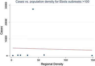
A scatter plot of the total number of cases against regional population density shows no obvious relationship between the population density of the area where the outbreak is initially discovered and the final number of cases.

Table 3.

Linear Effect from Initial Cases

	Estimate	SE	t value	Pr(> |t|)
Intercept	4985.72	5845.165	0.85	0.433
Initial Cases	− 7.671737	38.19996	− 0.2	0.849

Linear regression of final case count on initial case count demonstrates no linear relationship between initial reported case counts (independent variable) and final case counts (dependent variable).

Fig. 2.

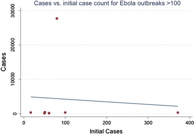
A scatter plot of total cases against initial cases at time of discovery shows no obvious relationship between the two. This implies that discovering an outbreak later is not necessarily tied to more final cases.

Economic Results

Table 4 indicates the discounted expected costs of an optimal SICP strategy are substantial (~ $10.5 billion), but the benefits (~ $18.5 billion) exceed these costs so that the expected net benefit of avoiding an outbreak is positive and quite large (~ $8 billion). Comparison of the steady-state values with the initial values indicates that much of the costs and benefits are borne over the longer run, although initial investment costs are large (10% of the present value of total costs over time). This highlights the fact that SICP is a long-run strategy that requires a large initial investment followed by smaller but continual annual expenditures in return for benefits that accrue over the far distant future. This means that short-sighted, reactive responses to disease outbreaks may be highly inefficient.

Table 4.

Simulation Results.

Scenario	Initial period valuesa				Steady-state valuesa
	Initial investment n(0)	Total costs − ρ2(0)	Net benefits of avoiding an outbreak, Z(0)	SICP capital stock N*	Investment n*	Total costs − ρ*2	Net benefits of avoiding an outbreak, Z*	Hazard rate ψ*
Baseline	1188	10,525	8040	1642	82	9171	7078	0.016
Sensitivity analysis b
1. Nmax = 10	1204	11,221	7252	1699	85	9840	6166	0.020
2. Nmax = 1	594	3752	19,570	706	35	3109	19,097	0.001
3. b* = 7%	1159	11,139	7607	1833	93	9760	5718	0.019
4. b* = 3%	1237	9448	8829	1324	69	8174	9614	0.012
5. Dmax and Dmin reduced 20%	991	9335	6558	1412	71	8189	5666	0.018
6. JX = Dmax for all N (No self-insurance)	1226	15,581	17,019	2185	110	13,929	18,671	0.010
7. JX(N) reduced by 90% for N = 5	1002	8629	5444	1347	68	7513	4699	0.019
8. α = 0.1	918	12,019	8390	1325	66	11,034	6746	0.020

Numerical results for the baseline scenario and eight alternative scenarios that illustrate the sensitivity of results to various parameters. For each case, we indicate the optimal initial investment, the present value of expected costs associated with the optimal pre-outbreak strategy, as well as the present value of expected net benefits from avoiding an outbreak. The remaining columns indicate steady-state values of the capital stock, investment levels required to offset depreciation and maintain the capital stock, steady-state costs and net benefits of the investment activities, and the steady-state hazard rate.

^aAll values except the hazard rate ψ are expressed in millions of US dollars. Costs and benefits are expected present values.

^bThe indicated parameter is changed as described, holding all other parameters at baseline values.

The baseline scenario indicates a large initial investment relative to the steady-state value of capital, N^*. The capital stock grows gradually for about 15–20 years after this initial investment before converging to its steady-state value, with investments declining during this period (Fig. 3a, b). These investments have the effect of driving the hazard rate well below the initial background level and keeping it there, even as the background hazard almost doubles over time (Fig. 3c). The hazard rate does increase as the background rate increases, but the SICP investments keep these increases small in comparison with changes in the background rate.

Fig. 3.

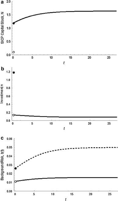
Time paths of key variables in the baseline scenario. The panels depict the time (t, shown on the horizontal axis) paths of the following variables in the cost-minimizing outcome prior to a future Ebola-like outbreak: a SICP capital stock, N, b investments, n, and c the hazard rate, ψ (solid), and background hazard rate, b (dashed). We assume initial capital stocks are negligible and that the initial background hazard rate is 2.6% and growing. Discontinuities at time t = 0 stem from a large initial investment in N (since N(0) = 0), which immediately increases N and decreases the hazard rate from the initial background level of b(0) = 0.026. After this initial investment, smaller investments in SICP are required to increase the capital stock as the background risk level increases to its steady-state value, after which investments only occur to offset the effects of depreciation. The investments mitigate the increased background hazard as the hazard rate remains much smaller than, and increase less quickly than, the background rate.

Of our eight sensitivity analyses (Table 4), scenarios 1 and 2 investigate the effect of different levels of investment required to eliminate risk, N^max. The larger the value of N^max, the less responsive is the hazard rate to SICP capital and the more expensive it becomes to manage outbreak risks. Our results indicate that a slightly larger value (~ 13.3% increase) leads to a small increase in optimal SICP investments, with total costs increasing and net benefits declining by a significantly larger amount due to the fact that an outbreak is more likely (e.g., the steady-state hazard rate has increased by 25% relative to the baseline). For the opposite case when lower levels of investment are required to eliminate risk in scenario 2 (a 90% decrease in N^max), investment is significantly more efficient and is reduced by 50% in the long-run, costs decline by 66%, and net benefits of avoiding an outbreak rise by 71%. These results suggest SICP investments are not very sensitive to small-to-moderate changes in N^max, but could be sensitive to extreme changes.

Scenarios 3 and 4 examine alternative values of the steady-state background hazard rate, b^*. Although these scenarios represent a 40% increase and decrease relative to the baseline value, investment levels, costs and net benefits do not change substantially. The results are not sensitive to changes in b^* (Table 4).

Scenario 5 examines a 25% across-the-board reduction in expected damage estimates associated with an outbreak. Here we find that investments and costs drop by about 12–15%, whereas the net benefits of SICP fall by 18–20%. These results suggest that optimal investment strategies and outcomes are fairly sensitive to the expected damages of an outbreak, as might be expected.

Scenarios 6 and 7 investigate the impact of self-insurance from capital investments. Specifically, scenario 6 investigates the extreme case where capital provides no self-insurance, whereas scenario 7 examines a case where self-insurance is more responsive to capital investments. In scenario 6 we find that investment increases substantially, particularly in the long run, to promote prevention (as indicated by the small steady-state hazard rate) since damages remain large in the absence of self-protection. Costs increase significantly, as do the benefits of avoiding an outbreak. The opposite occurs when SICP provides more self-insurance. These results indicate that self-insurance plays a significant role in formulating an optimal management strategy.

Finally, scenario 8 examines the role of larger maintenance or operating costs associated with SICP capital. In this scenario, we doubled the unit cost relative to the baseline. As expected, investment declines significantly while costs still increase relative to the baseline. The drop in investment results in a larger hazard rate, which increases the benefits of reducing an outbreak, at least at the onset of management. In the steady state, we find costs have increased so much that the benefits of avoiding an outbreak are reduced.

Discussion

Our epidemiological results suggest that the 2013–2015 W. African Ebola outbreak was not structurally different from other smaller Ebola virus disease outbreaks and that factors other than population density or immediacy of global alert (e.g., border movement issues) played a greater role in leading to significantly higher numbers of cases (Carroll et al. 2015; Kramer et al. 2016). This provides context to our economic model and informs the suggested policy response through how we think about the probability of future pandemic outbreaks. Models of the 2013–2015 epidemic’s early growth dynamics (Kiskowski 2014) suggest that we should expect no strong linear association between population density and final outbreak size. These models also lend weight to the notion that the proportion of outbreaks which are large may increase in the future. Community and household structure modulates the effect of population density on disease transmission (Kiskowski 2014). The stochastic nature of epidemics sees many (around 40%) initial outbreaks burn out with fewer than 150 cases. With small community mixing sizes (e.g., C = 5 outside-of-household contacts per individual), the distribution of epidemic size is skewed toward smaller numbers of cases. As community mixing size increases (representing more urbanized environments), the distribution of epidemic size becomes bimodal, with almost all epidemics which reach the survival threshold seeing over 1000 cases. This implies that while the 2013–2015 outbreak was not significantly different from past outbreaks, the increased interconnectedness of the area which it occurred in led to a larger overall outbreak. This is of course only one driver of the increased risk of an outbreak, and we can also consider land use change and climate change to be possible drivers. This is consistent with the 2013–2015 outbreak, where a major city (Conakry) was affected early in the outbreak [by the end of May 2014 when there were still less than 300 cases (World Health Organization 2014b)], whereas previous Ebola outbreaks were successfully contained in less densely populated areas. This may be because human populations at the region of origin have higher relative connectivity, pushing the virus more rapidly into urban areas (Wesolowski et al. 2014).

Our economic analysis suggests that US funding levels proposed and allocated after the Ebola outbreak may have been large enough to combat future threats (Tables 5 and 6). However, the portion of funding allocated to SICP remains unclear and may not adequately reflect the benefits of SICP. By contrast, the pandemic fund proposed by WHO is correctly positioned for SICP but woefully inadequate. We find that a standing capital prevention stock of $970 million could provide expected savings of $10.3 billion in reduced costs from avoiding expected future emerging disease impacts. Maintaining this stock at a steady state, however, would require annual investments of $48.5 million. That represents a significant amount of funding by donors, and one that would be politically challenging. We argue that this would be best structured as a pre-outbreak investment in strengthening existing SICP networks, e.g., through the WHO Global Outbreak Alert and Response Network (GOARN). This could involve strengthening GOARN to explicitly fund a reserve of mobile staff, equipment and laboratory capacity coupled with annual investments to maintain and expand this reserve over time. Staff and equipment could be deployed to leverage existing capacity in developing nations and emerging infectious disease hotspots (Allen et al. 2017). This also supports other calls for reform of national health capacities, including construction of a global health workforce reserve and investment in international health systems (Gostin and Friedman 2015).

Table 5.

Ebola Funding Allocations.

Ebola allocation
Department	Amount ($ in billions)
HHS	2.742
USAID and Department of State	2.5
Department of Defense	0.112
FDA	0.025
NIH	0.238

$6.18 billion was requested by the White House for Ebola emergency funding in November 2014 (The White House Office of the Press Secretary 2014). $5.4 billion was allocated by the US Congress (Mikulski 2015). The funding request included $4.6 billion for immediate response consisting of investments to fortify domestic public health systems, contain and mitigate the epidemic in West Africa, speed procurement and testing of vaccines and therapeutics and reduce the risk to Americans by building prevention and detection capacity in vulnerable countries. It also established a $1.54 billion contingency fund to ensure resources were available as the situation evolved, support domestic control efforts, expand monitoring, vaccinate healthcare workers and enhance global health security efforts. The funding that was actually allocated is shown below. All funds are immediately available for use, and none are held in a contingency fund.

Table 6.

Ebola Spending.

Health and Human Services Ebola Emergency Funding Spending Plan (Jan. 2015; Sylvia 2015).

Budget Activity	Amount (in billions)	Purpose
CDC	1.77	International and domestic response and preparedness; restore and strengthen capacities of health systems; build emergency operations centers; provide equipment and training to test patients; build capacities of laboratories to test specimens
Public Health and Social Services Emergency Fund	0.733	Develop and support research on Ebola vaccine and therapeutic candidates; hospital preparedness, equipment, training, care and transportation needs; reimburse domestic transportation and treatment costs for individuals treated in US for Ebola; procure necessary medical countermeasures
National Institutes of Health	0.238	Conduct clinical trials of vaccine candidates; discover new vaccines, therapeutics, and diagnostics
Food and Drug Administration	0.025	Conduct product review, development, and evaluation of Ebola vaccines; provide regulatory and scientific advice to stakeholders; develop medical devices and facilitate IVD development; facilitate clinical trials and product manufacturing; manage inter- and intra-agency activities related to Ebola; fund travel, lab supplies, and IT expenses; fund research for medical product safety, efficacy, and quality
Total	2.8

There is a clear need for greater clarity on the intended and final use of funds for pandemic prevention, and for more detailed analysis of their potential return-on-investment. The $5.4 Billion US Presidential budget request lacks clarity on how much funding was allocated to capacity building efforts, and the original request had $1.54 billion placed in a contingency fund for long-term efforts (The White House Office of the Press Secretary 2014). The Department of Health and Human Services released some details of their budget request, laying out a series of measures that addressed capacity building within the CDC allocation (Department of Health and Human Services 2015) (Tables 5 and 6). While this represented an advance toward building the preventive capital stock necessary for long-term Ebola prevention, without a direct commitment to development of a mobile outbreak prevention force and annual support to maintain this capacity, it was likely less than optimal. Our findings demonstrate the WHO’s proposed $100 million pandemic fund is too small to adequately prevent future Ebola outbreaks and supports analysis and call for reforms (Gostin and Friedman 2015).

Our economic modeling suggests a more effective way to allocate these resources is to maintain a fund large enough to allocate mobile resources during an outbreak and provide ongoing value between outbreaks. Previous articles have likened pandemic prevention to military activities (Time Inc 2015), and there has been a growing interest in, and funding to support global health threats as concomitant threats to security (Global Health Security Agenda 2018). While there are clear moral and ethical differences between wars and pandemics, this metaphor has economic cogency—for military and pandemic threats, investing in internationally-based rapidly deployable human resources coupled with strengthening of in-country infrastructure and capacity to curtail new events is economically optimal (Gostin and Friedman 2015). Defense departments use these approaches to counter global security threats. They create an overseas surge capacity (a ‘standing army’) and build alliances with partner nations, which include providing additional capacity to those partners. They also develop tactics to avoid redundancy in peace time. For EIDs, this could consist of trained responders based in regions prone to emerging diseases, with reservists stationed in donor countries. These international allies would be deployed first through networks like the Global Outbreak Alert and Response Network (GOARN)—with significantly improved capacity. In the West African Ebola outbreak, international aid funds were used to supply equipment and staff to enhance clinical and diagnostic capacity, to purchase personal protective equipment, increase biosecurity, and more rapidly develop and test vaccines and therapeutic agents (e.g., Butler 2014). These measures appear to have been ultimately successful. But without continued funding, capacity building investments depreciate over time, making them temporary in nature. In addition, if these resources were already deployed overseas before the outbreak, they may have been distributed faster.

This leads to a health economics dilemma: the strategy of responding to risks with a sudden increase in the flow of prevention spending—treating the control of the outbreak risk as a temporary flow that we can wait out—may be inadequate. A global pandemic fund, structured to produce a networked ‘standing army’ with international reservists to combat EIDs and to support ongoing costs of maintenance avoids this problem. This approach seems to reflect the goals of WHO GOARN (World Health Organization 2018). A straightforward solution to the pandemic threat may be a better-funded GOARN with a line item commitment for donor funding that cannot be significantly degraded between outbreaks or in global recessions, as seems to have occurred prior to the recent Ebola outbreak (Gostin and Friedman 2015; Heymann et al. 2015). This could be enhanced with a formal link to in-country programs that use development aid to build capacity to counter the pandemic threat (Gostin and Friedman 2015). Examples recently proposed include the FAO-OIE-WHO “One Health” approach to building biosecurity around livestock farms in countries where prior influenza outbreaks have originated (World Bank 2008), and the USAID “Emerging Pandemic Threats” program that targets novel and known emerging zoonoses in EID hotspots (Morse et al. 2012). While an international network of reservist experts would be needed to support this approach, a focus on building a standing army of local first-responders in at risk nations built around EID hotspots would logically provide the best allocation of resources. It also suggests that continued funding for global health security in countries at high risk of pandemic emergence could be a critical step to optimizing prevention and response to their threat (Global Health Security Agenda 2018).

The proposed levels of investment in our analysis should be taken as a lower bound. Many prevention activities that reduce the probability of an uncontrolled Ebola may also provide broader benefits to health and economic development. For instance, investment in prevention capital that includes hospitals can also provide healthcare services to local populations and build trust in local institutions—basic requirements for economic development. This would act as an additional benefit of capital, so that the optimal amount of investment in prevention rises until the total marginal benefit is equal to the marginal cost of funds. This could be a result of extending the focus from global health security to individual health security (Heymann et al. 2015). When we consider the impact of resources invested in affordable care in developing countries and the protection of developed nations, the benefits of prevention are greater, which suggests a strategy of even more investment.

Like major earthquakes or category 5 hurricanes, pandemics emerge stochastically from a background of frequent EID events that are predominantly zoonotic in nature and originate in tropical countries (Jones et al. 2008). These events are increasing in frequency as their underlying socioeconomic and environmental drivers expand (Jones et al. 2008). Furthermore, progressively globalized patterns of travel and trade result in an increasing risk of each new outbreak becoming a pandemic (Hosseini et al. 2010). This leads to a straightforward economic problem—there is an interval of time within which we must launch an effective global effort to pre-empt future events. If we wait too long, the probability of an outbreak accelerates and may lead to preemptive action being unfeasible or obsolete (Pike et al. 2014). Thus, while the deliberations on the size and nature of the WHO pandemic fund continue, the US government appropriation for Ebola response was used to combat to the outbreak of Zika virus, and depleted as a reserve for future pandemics. We therefore urge that a collective global strategy to combat future emerging disease threats is urgently formed, based on sound economic analysis, and focused on the countries where future emerging diseases are most likely to originate.

Appendix

Note that the current conditional Hamiltonian, henceforth called the Hamiltonian, in Eq. (6) represents a linear control problem. The optimal choice of n depends on the sign of its marginal value:

$$\frac{\partial H}{\partial n}=1+{\rho }_1\left\{\begin{array}{ccc}>0& \text{iff}& 0\\ =0& \text{iff}& n=n^{\ast }\\ <0& \text{iff}& n=\widehat{n}\end{array}\right.$$ A1

where n^* is the singular value of n (i.e., an interior, unconstrained solution). This condition says no investments should occur when the marginal benefit of SICP investments (− ρ₁) is less than the marginal cost of investment (unity), and investments should occur at a maximum level when the marginal benefit of SICP investments exceeds the marginal cost of investment. The singular solution should occur when the marginal benefits and costs of investment are equated.

The remaining necessary conditions for an optimum are given by the following adjoint conditions

$${\dot{\rho }}_1=\left[r+\psi \left(N,b\right)+\delta \right]{\rho }_1-C_N\left(N\right)-J{X}_N\left(N\right)\psi \left(N,b\right)-\left[JX\left(N\right)+{\rho }_2\right]{\psi }_N\left(N,b\right),$$ A2

$${\dot{\rho }}_2=\left[r+\psi \left(N,b\right)\right]{\rho }_2+n+C\left(N\right)+JX\left(N\right)\psi \left(N,b\right),$$ A3

$$\dot{\lambda }=\left[r+\psi \left(N,b\right)-{\sigma }_b\left(b\right)\right]\lambda -\left[JX\left(N\right)+{\rho }_2\right]{\psi }_b\left(N,b\right),$$ A4

and also the state equations. Together, conditions (A1)–(A4) and the state Eqs. (1), (2) and (5) determine cost-minimizing behavior through time.

Note that condition (A3) has the solution

$${\rho }_2=-\underset{t}{\overset{\infty }{\int }}\left(n+C\left(N\right)+JX\psi \left(N,b\right)\right)e^{-r\left(v-t\right)-y}\text{d}v.$$ A5

From (A5), − ρ₂ is the present value of expected costs, at time t, conditional on an outbreak having not yet occurred. Define Z = (JX(N) + ρ₂). This expression represents the difference between the certain costs of an outbreak (JX) and the expected costs continuing along the pre-outbreak prevention path (− ρ₂). Hence, Z is the expected increase in costs from transitioning from the pre-outbreak to post-outbreak state at time t. Alternatively, Z is the expected cost savings (i.e., a net benefit) from continuing along the pre-outbreak path as opposed to transitioning to the post-outbreak state. The term Z must be positive (Z > 0); otherwise the post-outbreak costs would be less than preventing an outbreak and it would be optimal to transition sooner. In what follows we treat Z as a state variable that changes over time according to

$$\begin{array}{cc}\hfill \dot{Z}& =J{X}_N\left(N\right)\dot{N}+{\dot{\rho }}_2\hfill \\ \hfill & =J{X}_N\left(N\right)\left[n-\delta N\right]+\left[r+\psi \left(N,b\right)\right]\left[Z-JX\left(N\right)\right]+n+C\left(N\right)+JX\left(N\right)\psi \left(N,b\right)\hfill \\ \hfill \end{array}$$ A6

We proceed by examining the singular solution. In this case, (A1) yields

$$-{\rho }_1=1$$ A7

Time differentiating this condition yields ${\dot{\rho }}_1=0$. Substituting this result into adjoint condition (A2) leads to the relation

$$1=\frac{-{\psi }_N\left(N,b\right)Z-J{X}_N\left(N\right)\psi \left(N,b\right)-C_N\left(N\right)}{r+\psi \left(N,b\right)+\delta }.$$ A8

The LHS is the marginal cost of investment in SICP and provides the measuring stick against which the marginal benefits of investment in prevention must be weighed. The cost-minimizing solution requires marginal costs to equal the annuity value of the net marginal benefits of the prevention stock (RHS) using a risk- and depreciation-adjusted discount factor. The net marginal benefits (the RHS numerator) include the expected reduced marginal cost of an outbreak due to a reduction in the likelihood of an outbreak (− ψ_N(N, b)Z) and reduced damages due to self-protection (− JX_N(N)ψ(N, b)), less the marginal maintenance cost of SICP capital. Condition (A8) implicitly defines the singular value of Z as

$$Z\left(N,b\right)=\frac{r+\psi \left(N,b\right)+\delta +J{X}_N\left(N\right)\psi \left(N,b\right)+C_N\left(N\right)}{-{\psi }_N\left(N,b\right)}$$ A9

which is a feedback response to the states N and b. Time differentiating this relation and setting it equal to (A6) yields

$$\begin{array}{c}\hfill J{X}_N\left(N\right)\left[n-\delta N\right]+\left[r+\psi \left(N,b\right)\right]\left[Z\left(N,b\right)-JX\left(N\right)\right]+n+C\left(N\right)\\ \hfill +JX\left(N\right)\psi \left(N,b\right)=Z_N\left[n-\delta N\right]+Z_b\sigma \left(b\right)\\ \hfill \end{array}$$ A10

Condition (A10) can be solved for the singular value of n as the feedback relation

$$n\left(N,b\right)=\delta N+\frac{\left(rJX\left(N\right)-\delta N-\left[r+\psi \left(N,b\right)\right]Z\left(N,b\right)-C\left(N\right)\right)+Z_b\left(N,b\right)\sigma \left(b\right)}{1+J{X}_N\left(N\right)-Z_N\left(N,b\right)}$$ A11

The dynamics of the optimized system are determined by the system

$$\dot{b}=\sigma \left(b\right),\text{and}\dot{N}=n\left(N,b\right)-\delta N,$$ A12

where the new state equation for N is obtained by substituting in the feedback rule for n into the original state equation. The dynamics in (A12) provide insight into the singular value n(N,b). Specifically, n(N,b) equals its steady-state value δN plus an adjustment term reflecting the fact that, away from the steady state with σ(b) = 0, b changes over time. Changes in b generate two effects arising in the numerator of the second RHS term in (A11). Using the approach outlined in “Appendix” from (29), the first term in the numerator (in parentheses) equals the value of changes in b, which is λσ(b). The second term in the numerator is the effect of changes in b on the singular value of Z. These numerator terms vanish in the steady state with n = δN and σ(b) = 0. In particular, the first RHS numerator term in (A11) vanishes to yield:

$$Z\left(N,b\right)=\frac{rJX\left(N\right)-\left[\delta N+C\left(N\right)\right]}{r+\psi \left(N,b\right)}.$$ A13

The RHS numerator of condition (A13) is the flow value of damages, rJX(N), less the costs of SICP investment and maintenance prior to the outbreak, δN + C(N). The denominator is a risk-adjusted discount rate. The RHS is the risk-adjusted perpetuity value of cost savings from avoiding an outbreak. Condition (A13) says this perpetuity value optimally equals the steady-state net cost savings from avoiding an outbreak, Z(N,b).

The dynamics can be explored more fully by drawing a phase plane in (N,b) space, presented in Figure 4 for the baseline scenario. We begin by defining the isoclines associated with the singular solution. The $\dot{b}=0$ isocline is σ(b) = 0, which is a horizontal line. The $\dot{N}=0$ isocline is defined by setting the RHS numerator in (A11) equal to zero. Individually, these isoclines indicate where the indicated state variable is unchanging, given the current value of the other state variable. A steady state for both state variables occurs at the intersection of the isoclines. Off the isoclines, movement occurs as directed by the phase arrows. Figure 1a indicates there is a single steady state, at point P, which found numerically (i.e., using eigenvalues) to be a saddle point equilibrium. The singular solution consists of separatrices (also known as a saddle path), labeled p, to the steady state.

Fig. 4.

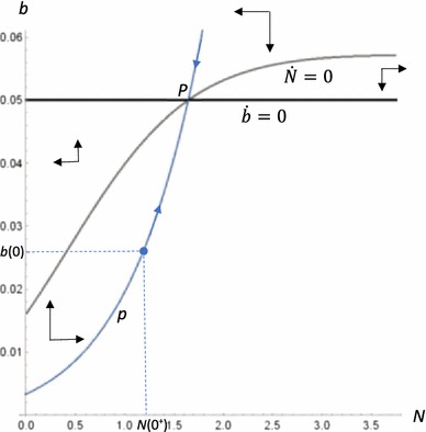
Phase plane for the baseline scenario. The phase plane depicts the dynamics of how the variables N and b move together over time (where N is expressed in billions of US dollars). The intersection of the $\dot{N}=0$ and $\dot{b}=0$ isoclines produces a saddle point steady-state equilibrium at point P, which is optimally pursued by following path p. Given the initial value of b(0) = 0.026, the initial investment n(0) should be made to bring the capital stock up to N(0⁺). Future investments should then be made to keep N on path p as b increases over time.

We assume the initial value of b is 0.026, as indicated by b(0) on the phase plane. We also assume in our numerical analyses that N(0) = 0. This means an initial investment of N(0⁺) is required, which moves us to the indicated point on the saddle path p. Once on path p, the optimal strategy is to remain on the path. This involves making investments n to adjust N to stay on the path as b changes over time.

References

- Allen T, Murray KA, Zambrana-Torrelio C, Morse SS, Rondinini C, Di Marco M, et al. Global hotspots and correlates of emerging zoonotic diseases. Nature Communications. 2017;8:1124. doi: 10.1038/s41467-017-00923-8. [DOI] [PMC free article] [PubMed] [Google Scholar]
- Berry K, Finnoff D, Horan R, Shogren JF. Managing the endogenous risk of disease outbreaks. Journal of Economic Dynamics and Control. 2015;51:166–179. doi: 10.1016/j.jedc.2014.09.014. [DOI] [PMC free article] [PubMed] [Google Scholar]
- Butler D. Global Ebola response kicks into gear at last. Nature. 2014;513:469. doi: 10.1038/513469a. [DOI] [PubMed] [Google Scholar]
- Carroll MW, Matthews DA, Hiscox JA, Elmore MJ, Pollakis G, Rambaut A, et al. Temporal and spatial analysis of the 2014–2015 Ebola virus outbreak in West Africa. Nature. 2015;524:U97–U201. doi: 10.1038/nature14594. [DOI] [PMC free article] [PubMed] [Google Scholar]
- Centers for Disease Control and Prevention (2014) Outbreaks Chronology: Ebola Virus Disease http://www.cdc.gov/vhf/ebola/outbreaks/history/chronology.html. Accessed on December 17th, 2014
- Collin N, de Radiguès X, World Health Organization HNVTF Vaccine production capacity for seasonal and pandemic (H1N1) 2009 influenza. Vaccine. 2009;27:5184–5186. doi: 10.1016/j.vaccine.2009.06.034. [DOI] [PubMed] [Google Scholar]
- Department of Health and Human Services (2015) Ebola Emergency Funding Spend Plan
- Global Health Security Agenda (2018) Global Health Security Agenda https://www.ghsagenda.org/. Accessed on Feb 20th 2018, 2018
- Gostin LO, Friedman EA. A retrospective and prospective analysis of the west African Ebola virus disease epidemic: robust national health systems at the foundation and an empowered WHO at the apex. Lancet. 2015;385:1902–1909. doi: 10.1016/S0140-6736(15)60644-4. [DOI] [PubMed] [Google Scholar]
- Heymann DL, Chen L, Takemi K, Fidler DP, Tappero JW, Thomas MJ, et al. Global health security: the wider lessons from the west African Ebola virus disease epidemic. Lancet. 2015;385:1884–1901. doi: 10.1016/S0140-6736(15)60858-3. [DOI] [PMC free article] [PubMed] [Google Scholar]
- Hosseini P, Sokolow SH, Vandegrift KJ, Kilpatrick AM, Daszak P. Predictive power of air travel and socio-economic data for early pandemic spread. PLoS ONE. 2010;5:e12763. doi: 10.1371/journal.pone.0012763. [DOI] [PMC free article] [PubMed] [Google Scholar]
- International Commission Ebola hemorrhagic fever in Zaire, 1976. Bulletin of the World Health Organization. 1978;56:271–293. [PMC free article] [PubMed] [Google Scholar]
- Jones KE, Patel NG, Levy MA, Storeygard A, Balk D, Gittleman JL, et al. Global trends in emerging infectious diseases. Nature. 2008;451:990–993. doi: 10.1038/nature06536. [DOI] [PMC free article] [PubMed] [Google Scholar]
- Kaput VM (2007) Declaration fin d’epidemie de FHV a virus Ebola dans les zones de sante de Mweka, Bulape et Luebo, Province du Kasai Occidental, RD Congo. République démocratique du Congo
- Keegan R, Dabbagh A, Strebel PM, Cochi SL. Comparing measles with previous eradication programs: enabling and constraining factors. Journal of Infectious Diseases. 2011;204:S54–S61. doi: 10.1093/infdis/jir119. [DOI] [PubMed] [Google Scholar]
- Khan AS. Public health preparedness and response in the USA since 9/11: a national health security imperative. The Lancet. 2011;378:953–956. doi: 10.1016/S0140-6736(11)61263-4. [DOI] [PMC free article] [PubMed] [Google Scholar]
- Khan AS, Tshioko K, Heymann DL, Guenno BL, Nabeth P, Kerstiens B, et al. The reemergence of Ebola hemorrhagic fever, Democratic Republic of the Congo, 1995. Commission de Lutte contre les Epidémies à Kikwit. J Infect Dis. 1999;179:S76–S86. doi: 10.1086/514306. [DOI] [PubMed] [Google Scholar]
- Kiskowski M (2014) A three-scale network model for the early growth dynamics of 2014 West Africa Ebola epidemic. PLoS currents [DOI] [PMC free article] [PubMed]
- Kramer AM, Pulliam JT, Alexander LW, Park AW, Rohani P, Drake JM. Spatial spread of the West Africa Ebola epidemic. Royal Society Open Science. 2016;3:11. doi: 10.1098/rsos.160294. [DOI] [PMC free article] [PubMed] [Google Scholar]
- Lee K. Risk aversion and self-insurance-cum-protection. Journal of Risk and Uncertainty. 1998;17:139–150. doi: 10.1023/A:1007719629165. [DOI] [Google Scholar]
- MacNeil A, Farnon EC, Morgan OW, Gould P, Boehmer TK, Blaney DD, et al. Filovirus outbreak detection and surveillance: lessons from Bundibugyo. J Infect Dis. 2011;204:S761–S767. doi: 10.1093/infdis/jir294. [DOI] [PubMed] [Google Scholar]
- Mikulski BA (2015) Summary: Fiscal Year 2015 omnibus appropriations bill. in C. o. Appropriations, editor. United States Senate, http://www.appropriations.senate.gov/news/summary-fiscal-year-2015-omnibus-appropriations-bill
- Morens DM, Folkers GK, Fauci AS. The challenge of emerging and re-emerging infectious diseases. Nature. 2004;430:242–249. doi: 10.1038/nature02759. [DOI] [PMC free article] [PubMed] [Google Scholar]
- Morse SS, Mazet JAK, Woolhouse M, Parrish CR, Carroll D, Karesh WB, et al. Prediction and prevention of the next pandemic zoonosis. The Lancet. 2012;380:1956–1965. doi: 10.1016/S0140-6736(12)61684-5. [DOI] [PMC free article] [PubMed] [Google Scholar]
- Okware SI, Omaswa FG, Zaramba S, Opio A, Lutwama JJ, Kamugisha J, et al. An outbreak of Ebola in Uganda. Tropical Medicine & International Health. 2002;7:1068–1075. doi: 10.1046/j.1365-3156.2002.00944.x. [DOI] [PubMed] [Google Scholar]
- Orellana C. WHA adopts new International Health Regulations. The Lancet Infectious Diseases. 2005;5:402. doi: 10.1016/S1473-3099(05)70153-5. [DOI] [Google Scholar]
- Pike J, Bogich TL, Elwood S, Finnoff DC, Daszak P. Economic optimization of a global strategy to reduce the pandemic threat. Proceedings of the National Academy of Sciences, USA. 2014;111:18519–18523. doi: 10.1073/pnas.1412661112. [DOI] [PMC free article] [PubMed] [Google Scholar]
- Reed WJ, Heras HE. The conservation and exploitation of vulnerable resources. Bulletin of Mathematical Biology. 1992;54:185–207. doi: 10.1007/BF02464829. [DOI] [Google Scholar]
- Reuters (2015) WHO boss Chan launches $100 million health emergency fund http://www.reuters.com/article/2015/05/18/us-health-ebola-chan-idUSKBN0O31E620150518. Accessed on May 31st 2015
- Sylvia B (2015) Ebola Emergency Funding Spend Plan. Department of Health and Human Services
- The White House Office of the Press Secretary (2014) Fact Sheet: Emergency Funding Request to Enhance the U.S. Government’s Response to Ebola at Home and Abroad. Office of the Press Secretary
- Time Inc. (2015) Bill Gates Says We Must Prepare for Future Pandemics as for ‘War’ http://time.com/3685490/bill-gates-ebola-pandemics/. Accessed on May 31st 2015, 2015
- Walley T, Davidson P. Research funding in a pandemic. The Lancet. 2010;375:1063–1065. doi: 10.1016/S0140-6736(10)60068-2. [DOI] [PubMed] [Google Scholar]
- Wesolowski A, Buckee CO, Bengtsson L, Wetter E, Lu X, and Tatem AJ (2014) Commentary: containing the Ebola outbreak—the potential and challenge of mobile network data. PLoS Currents Outbreaks 1 [DOI] [PMC free article] [PubMed]
- WHO/International Study Team Ebola haemorrhagic fever in Sudan, 1976. Report of a WHO/International Study Team. Bulletin of the World Health Organization. 1978;56:247–270. [PMC free article] [PubMed] [Google Scholar]
- World Bank (2008) Contributing to One World, One Health: a strategic framework for reducing risks of infectious diseases at the animal-human-ecosystems interface. Food and Agriculture Organization; World Organisation for Animal Health; World Health Organization; United Nations System Influenza Coordinator; United Nations Children’s Fund; World Bank, Rome
- World Bank Group (2014) Update on the economic impact of the 2014 Ebola epidemic on Liberia, Sierra Leone, and Guinea. World Bank
- World Health Organization (2004) Republic of the Congo: Ebola Outbreak. http://www.who.int/emergencies/ebola-DRC-2017/en/
- World Health Organization (2014a) Ebola virus disease fact sheet http://www.who.int/mediacentre/factsheets/fs103/en/
- World Health Organization (2014b) Ebola Virus Disease, West Africa (Situation as of 2 May 2014) http://www.afro.who.int/en/clusters-a-programmes/dpc/epidemic-a-pandemic-alert-and-response/outbreak-news/4130-ebola-virus-disease-west-africa-2-may-2014.html. Accessed on March 1st 2015
- World Health Organization (2015a) Ebola Situation Reports http://apps.who.int/ebola/en/current-situation/ebola-situation-report. Accessed on March 25th 2015
- World Health Organization (2015b) Report of the Ebola Interim Assessment Panel
- World Health Organization (2018) Global Outbreak Alert and Response Network (GOARN) http://www.who.int/csr/outbreaknetwork/en/. Accessed on February 15th 2018