Pattern formation of an epidemic model with diffusion

Abstract

One subject of spatial epidemiology is spatial variation in disease risk or incidence. The spread of epidemics can result in strong spatial patterns of such risk or incidence: for example, pathogen dispersal might be highly localized, vectors or reservoirs for pathogens might be spatially restricted, or susceptible hosts might be clumped. Here, spatial pattern of an epidemic model with nonlinear incidence rates is investigated. The conditions for Hopf bifurcation and Turing bifurcation are gained and, in particular, exact Turing domain is found in the two parameters space. Furthermore, numerical results show that force of infection, namely β, plays an important role in the spatial pattern. More specifically, different patterns emerge as β increases. The mathematical analysis and numerical results well extend the finding of pattern formation in the epidemic models and may well explain the field observed in some areas.

Introduction

Over the past decade, there has been renewed public and official concern about infectious disease as a major public health threat. Indeed, the concern has arisen against a background of some surprise. In the past quarter of a century, we have encountered the emergence of Legionnaire’s disease, Lyme disease, HIV/AIDS, Ebola virus, human mad cow disease, the Nipah virus, West Nile fever and SARS, as well as resurgent adversaries such as tuberculosis, cholera, dengue fever, and malaria [1].

Since emerging infectious diseases are a growing agent of global change that present compelling challenges in public health, agriculture, and wildlife management [2–5], predicting the spread of an infectious disease depends on understanding the spatiotemporal dynamics of an epidemic model. On the other hand, the understanding of the spread of epidemics has become a goal in itself because, as well as possessing complex dynamics, it has a very simple natural history and, therefore, many plausible population models [6].

Most researchers pay their attention to the temporal development of epidemics. However, many important epidemiological phenomena are strongly influenced by space because of the localized nature of transmission or other forms of interaction [7–12]. The spread of invading organisms [13, 14] is very important and recent events have focused attention on the spread of human, livestock, crop, and wildlife diseases [15–19]. As a result, mathematical models with time and space are useful in investigating the process of epidemic spreading. Epidemic wavefronts may be found in reaction–diffusion models, which were observed in the real world, such as in the spread of the Black Death in Europe from 1347 to 1350 [20–22].

The studies presented in this paper want to know that how populations diseases transmit in both space and time, which can enhance the understanding of the epidemiological features of diseases in the populations. To this end, we will investigate pattern formation of a spatial SI model with nonlinear incidence rates in this paper. More specifically, we will reveal that how force of infection, namely β, has influence on the distribution of the infected populations.

Model

To begin this section, we firstly give two main assumptions, which are as follows.

(i) The population, in which a pathogenic agent is active, comprises two subgroups: the healthy individuals who are susceptible (S) to infection and the already infected individuals (I) who can transmit the disease to the healthy ones. Both S and I are functions of time.

(ii) The disease-related death rate from the infected is d and the natural death rate of both the suspectable and the infected is μ.

Liu et al. [23, 24] concluded that the bilinear mass action incidence rate due to saturation or multiple exposures before infection could lead to nonlinear incidence rate βS ^p I ^q. Therefore, the incidence rate is assumed to be nonlinear βS ^p I ^q without a periodic forcing which has much wider range of dynamical behaviors in comparison to bilinear incidence rate βSI. Here, β is the force of infection or the rate of transmission. Simple case, by their own nature, cannot incorporate many of the complex biological factors. However, they often provide useful insights to help our understanding of complex process [25–27]. Thus, in the present paper, we set p=1 and q=2.

The model we employ is as follows:

1a

1b

where A is the recruitment rate of the population, d is the natural death rate of the population, and μ is the disease-related death rate from the infected. x and y mean the space. Here, ∇²=∂ ²/∂x ²+∂ ²/∂y ² is the usual Laplacian operator in two-dimensional space and D ₁, D ₂ are, respectively, the susceptible and infected individuals diffusion coefficients. From the biological point of view, we assume all the parameters are positive throughout the paper.

The model (1a), (1b) needs to be analyzed with the initial populations

and the boundary conditions

2

where n is space, (x,y)∈∂Ω and Ω is the spatial domain.

Bifurcation analysis

In order to provide Turing instability of the reaction-diffusion system, it is important to consider the local dynamics of the system [28]. The corresponding nondiffusion model is

3a

3b

The dynamics in the biologically meaningful region S≥0, I≥0 are of interest. By considering the nullclines f=0, g=0, and the intersection of these curves in phase space, we give the linear stability analysis of the system. Simple calculations show that the system (3a), (3b) has three equilibrium points:

• (i) , which is corresponding to extinction of the epidemic
• (ii)
  

  which is corresponding to the coexistence of the S and I
• (iii)
  

  which is corresponding to the coexistence of the S and I.

By direct calculations, we know that E ₂ is unstable, which is a saddle. Thus, we are interested to study the stability behavior of the interior equilibrium point E ^∗. The Jacobian corresponding to this equilibrium point is that

where

and

Following the standard linear analysis of the reaction–diffusion equation [20, 29], we address the temporal stability of the uniform states which is associated with nonuniform perturbations

4

where λ is the perturbation growth rate, k is the wavenumber, and c.c. stands for complex conjugate. The linear instability (θ≪1) of each one of the uniform states, is deduced from the dispersion relations. Substituting expression (4) into (1a), (1b) and neglecting all nonlinear terms in S and I, we obtain that the eigenvalue is the root of the following equation:

5

where

6a

6b

Therefore, the solution of (5) reduces to

7

The reaction–diffusion systems have led to the characterization of three basic types of symmetry-breaking bifurcations responsible for the emergence of spatiotemporal patterns. The onset of Hopf instability corresponds to the case, when a pair of imaginary eigenvalues cross the real axis from the negative to the positive side. And this situation occurs only when the diffusion vanishes [30, 31]. Mathematically speaking, the Hopf bifurcation occurs when

8

Then we can get the critical value of the transition, Hopf bifurcation parameter—β, equals to that

9

Turing bifurcation occurs when

10

with

11

By direct calculation, we can obtain the critical value of bifurcation parameter β equals

where

Now, let us discuss the bifurcations represented by these formulas in the parameter space spanned by the parameters β and μ which can be seen from Fig. 1. The whole class of the spatial model is included in this parameter space. The upper part of the displayed parameter space (where is marked by IV) corresponds to systems with homogeneous equilibria, which is unconditionally stable. If this region is left via a bifurcation (Turing or Hopf), the qualitative behavior of such equilibria changes. If an equilibrium is represented by a point in the part of the parameter space, where is marked by I, it can be destabilized by a homogeneous oscillations. In Domain II, both Hopf and Turing instability occur. The equilibria that can be found in the area, where is marked by III, is stable with respect to homogeneous perturbations but loose their stability with respect to perturbations of specific wave numbers k. In this region, stationary inhomogeneous patterns can be observed. Figure 2 shows the real part of the character value of (7) as β increases.

Fig. 1.

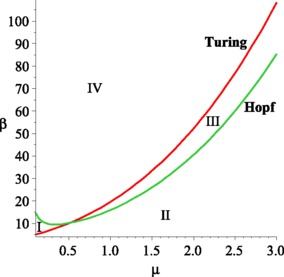
(Color online) Bifurcation diagram of model (1a), (1b). We set the parameter values are A=1, d=1, D ₁=6, and D ₂=1. The figure shows the Turing space (where is marked by III) which is the area bounded by the Turing bifurcation line (the red one) and the Hopf bifurcation line (the green one)

Fig. 2.

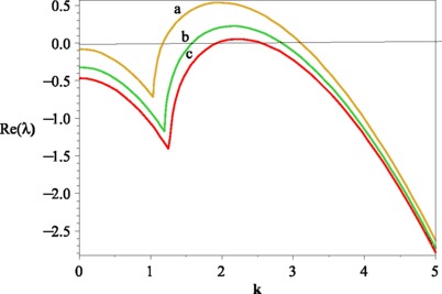
(Color online) The real part of the character value as p is increased. We set the parameter values are that A=1, μ=1.8, d=1, D ₁=6, and D ₂=1. And the values of β are that a: β=35; b: β=38; c: β=40

Main results

Since the dynamical behavior of the spatial model cannot be studied by using analytical methods or normal forms, we have to perform numerical simulations by computer. The continuous problem defined by the reaction-diffusion system in two-dimensional space is solved in a discrete domain with M×N lattice sites. The space between the lattice points is defined by the lattice constant Δh. The time evolution is also discrete, i.e., the time goes in steps of Δt. The time evolution can be solved by using the Euler method. In the present paper, we set Δh=1, Δt=0.01 and M=N=200. And it was also checked that a further decrease of the step values did not lead to any significant modification of the results.

In the following, we will perform a series of numerical simulations of the spatially extended model (1a), (1b) in two-dimensional spaces, and the qualitative results are shown by figures. We keep A=1, μ=1.8, d=1, D ₁=6, and D ₂=1 and β is regarded as a parameter. All our numerical simulations are employed with a system size of 200×200 space units. We run the simulations until they reach a stationary state or until they show a behavior that does not seem to change its characteristics anymore. In this paper, we want to know the distribution of the infected. As a result, we can restrict our analysis of pattern formation of I.

Figure 3 shows the evolution of the spatial pattern of infected population at 0, 500, 20,000, and 50,000 iterations, with small random perturbation of the stationary solution S ^∗ and I ^∗ of the spatially homogeneous systems when the parameter values are in the domain of Turing space. In this case, one can see that for the model (1a), (1b), the random initial distribution leads to the formation of a strongly irregular transient pattern in the domain. After the irregular pattern forms, it grows slightly and jumps alternately for a certain time, and finally the network-like patterns prevail over the whole domain, and the dynamics of the system does not undergo any further changes. These patterns are different from the previous results [31, 32].

Fig. 3.

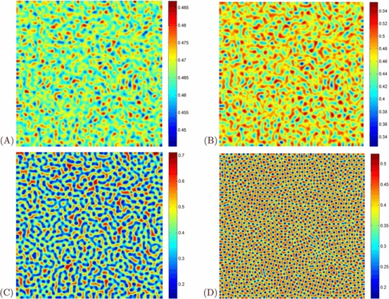
(Color online) Snapshots of contour pictures of the time evolution of the I at different instants with A=1, μ=1.8, d=1, D ₁=6, and D ₂=1, and β=32, which are in the Turing space. (A): 0 iteration; (B): 500 iterations; (C): 20,000 iterations and (D): 50,000 iterations

The parameter values of Figs. 4–5 are in the domain of Turing space. All of the figures show the evolution of the spatial pattern of the at 10, 1,000, 10,000 and 100,000 iterations, with small random perturbation of the stationary solution S ^∗ and I ^∗ of the spatially homogeneous systems. From Figs. 4–5, we can see that the regular stripe patterns prevail over the whole domain at last, and the dynamics of the system does not undergo any further changes. Note that although the dynamics of the system starts from the same initial condition as previous cases, there is an essential difference for the spatially extended model. Specifically, the direction of the stripe of the two figures are different.

Fig. 4.

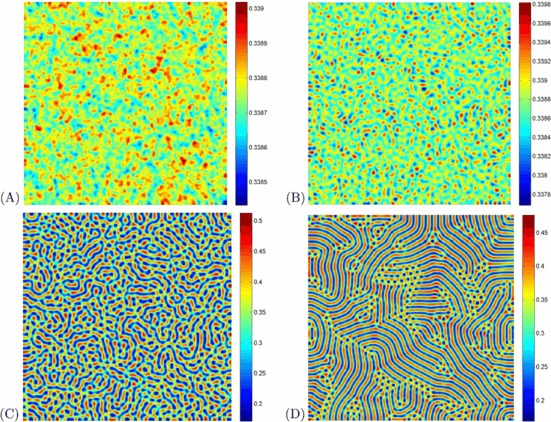
(Color online) Snapshots of contour pictures of the time evolution of the I at different instants with A=1, μ=1.8, d=1, D ₁=6, and D ₂=1, and β=35, which are in the Turing space. (A): 10 iterations; (B): 1,000 iterations; (C): 10,000 iterations and (D): 100,000 iterations

Fig. 5.

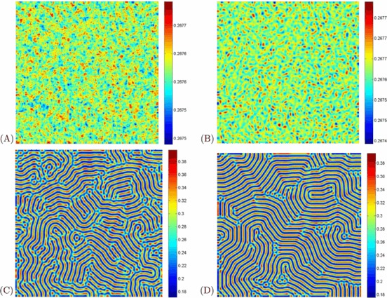
(Color online) Snapshots of contour pictures of the time evolution of the I at different instants with A=1, μ=1.8, d=1, D ₁=6, and D ₂=1, and β=40, which are in the Turing space. (A): 10 iterations; (B): 1,000 iterations; (C): 10,000 iterations and (D): 100,000 iterations

Figure 6 shows that stationary stripe and spot patterns emerge mixed in the distribution of the infected population density. After the stripe-like patterns form, they grow steadily with time until they reach certain arm length, and the spatial patterns become distinct. Finally, the spotted spatial patterns prevail the whole domain and the dynamics of the system does not undergo any further changes.

Fig. 6.

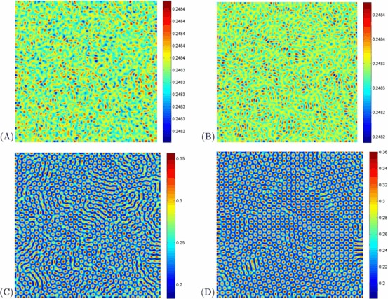
(Color online) Snapshots of contour pictures of the time evolution of the I at different instants with A=1, μ=1.8, d=1, D ₁=6, and D ₂=1, and β=42, which are in the Turing space. (A): 10 iterations; (B): 1,000 iterations; (C): 10,000 iterations and (D): 100,000 iterations

Discussion and conclusion

From the analysis in Sect. 3 and the above figures, we can see that the numerical results correspond perfectly to our theoretical findings, that is to say, there are a range of parameters where different spatial patterns emerge. More specifically, typical dynamics of population density variation, i.e., stripe-like or spotted or coexistence of both, which are the formation of isolated groups are obtained.

If considered in a somewhat broader epidemic perspective, our results have an intuitively clear meaning. There has been a growing understanding during the past years that, what transitions between different dynamical regimes arising as a result of perturbation of the system’s parameters [33]. From this standpoint, it seems interesting to know how the dynamics varies when the parameters move across the diagram [34]. For simplicity, let us assume that only one parameter is changing, such as β, others remaining fixed. An increase of the β plays an important role in the pattern formation. More specifically, stripe only, coexistence of stripe and spotted, and spotted only emerge successively.

In [31], we investigated a spatial SI model with logistic growth and nonlinear incidence rates βS ^p I ^q with p+q=1. However, in this paper, we assume the population grows with constant rate and set p=1 and q=2. Moreover, in the previous paper [29–31], we did not focus our attention on the infection rate which may have great influence on pattern formations of disease and we reveal it by numerical simulations in the present paper.

To explain spatial patterns arising from the spatial epidemic model in the real world, here we present some observations of the spatial and temporal dynamics of hantavirus pulmonary syndrome during the 1990s. In [35], it shows spatial patterns of location of hantavirus pulmonary syndrome in southwestern USA. Our results well capture some key features of the complex variation and explain the observation in spatial structure to most species by comparing Figs. 3–6 with the pictures in [35]. In other words, modeling the epidemics using reaction-diffusion form can help us understand the distribution of disease in both time and space.

References

- 1.McMichael A.J. Environmental and social influences on emerging infectious diseases: past, present and future. Philos. Trans. R. Soc. Lond. B, Biol. Sci. 2004;359:1049–1058. doi: 10.1098/rstb.2004.1480. [DOI] [PMC free article] [PubMed] [Google Scholar]
- 2.Keeling M.J., Woolhouse M.E.J., Shaw D.J., Matthews L., Chase-Topping M., Haydon D.T., Cornell S.J., Kappey J., Wilesmith J., Grenfell B.T. Dynamics of the 2001 UK foot and mouth epidemic: stochastic dispersal in a heterogeneous landscape. Science. 2001;294:813–817. doi: 10.1126/science.1065973. [DOI] [PubMed] [Google Scholar]
- 3.Blower S.M., McLean A.R. Mixing ecology and epidemiology. Proc. R. Soc. Lond. B, Biol. Sci. 1991;245:187–192. doi: 10.1098/rspb.1991.0108. [DOI] [PubMed] [Google Scholar]
- 4.Binder S., Levitt A.M., Sacks J.J., Hughes J.M. Emerging infectious diseases: public health issues for the 21st century. Science. 1999;284:1311–1313. doi: 10.1126/science.284.5418.1311. [DOI] [PubMed] [Google Scholar]
- 5.Wonham M.J., de-Camino-Beck T., Lewis M.A. An epidemiological model for West Nile virus: invasion analysis and control applications. Proc. R. Soc. Lond. B, Biol. Sci. 2004;271:501–507. doi: 10.1098/rspb.2003.2608. [DOI] [PMC free article] [PubMed] [Google Scholar]
- 6.Keeling M.J., Rand D.A., Morris A.J. Correlation models for childhood diseases. Proc. R. Soc. Lond. B, Biol. Sci. 1997;264:1149–1156. doi: 10.1098/rspb.1997.0159. [DOI] [PMC free article] [PubMed] [Google Scholar]
- 7.Smith D.L., Lucey B., Waller L.A., Childs J.E., Real L.A. Predicting the spatial dynamics of rabies epidemics on heterogeneous landscapes. Proc. Natl. Acad. Sci. USA. 2002;99:3668–3672. doi: 10.1073/pnas.042400799. [DOI] [PMC free article] [PubMed] [Google Scholar]
- 8.Keeling M.J., Woolhouse M.E.J., May R.M., Davies G., Grenfell B.T. Modelling vaccination strategies against foot-and-mouth disease. Nature. 2003;421:136–142. doi: 10.1038/nature01343. [DOI] [PubMed] [Google Scholar]
- 9.Hufnagel L., Brockmann D., Geisel T. Forecast and control of epidemics in a globalized world. Proc. Natl. Acad. Sci. USA. 2004;101:15124–15129. doi: 10.1073/pnas.0308344101. [DOI] [PMC free article] [PubMed] [Google Scholar]
- 10.Riley S., Ferguson N.M. Smallpox transmission and control: Spatial dynamics in Great Britain. Proc. Natl. Acad. Sci. USA. 2006;103:12637–12642. doi: 10.1073/pnas.0510873103. [DOI] [PMC free article] [PubMed] [Google Scholar]
- 11.Hanski I. Coexistence of competitors in patchy environment. Ecology. 1983;64:493–500. doi: 10.2307/1939969. [DOI] [Google Scholar]
- 12.Hastings A. Spatialheterogeneity and ecological models. Ecology. 1990;71:426–428. doi: 10.2307/1940296. [DOI] [Google Scholar]
- 13.Kot M., Lewis M.A., Driessche P.v.d. Dispersal data and the spread of invading organisms. Ecology. 1996;77:2027–2042. doi: 10.2307/2265698. [DOI] [Google Scholar]
- 14.Sun G.-Q., Jin Z., Liu Q.-X., Li L. Spatial pattern in an epidemic system with cross-diffusion of the susceptible. J. Biol. Syst. 2009;17:141–152. doi: 10.1142/S0218339009002843. [DOI] [Google Scholar]
- 15.Gani R., Leach S. Transmission potential of smallpox in contemporary populations. Nature. 2001;414:748–751. doi: 10.1038/414748a. [DOI] [PubMed] [Google Scholar]
- 16.Dye C., Gay N. Modeling the SARS epidemic. Science. 2003;300:1884–1885. doi: 10.1126/science.1086925. [DOI] [PubMed] [Google Scholar]
- 17.Lonsdale W.M. Global patterns of plant invasions and the concept of invasibility. Ecology. 1999;80:1522–1536. doi: 10.1890/0012-9658(1999)080[1522:GPOPIA]2.0.CO;2. [DOI] [Google Scholar]
- 18.Ferguson N.M., Keeling M.J., Edmunds W.J., Gani R., Grenfell B.T., Anderson R.M., Leach S. Planning for smallpox outbreaks. Nature. 2003;425:681–685. doi: 10.1038/nature02007. [DOI] [PMC free article] [PubMed] [Google Scholar]
- 19.Keeling M.J., Brooks S.P., Gilligan C.A. Using conservation of pattern to estimate spatial parameters from a single snapshot. Proc. Natl. Acad. Sci. USA. 2004;101:9155–9160. doi: 10.1073/pnas.0400335101. [DOI] [PMC free article] [PubMed] [Google Scholar]
- 20.Murray J.D. Mathematical Biology. 3. Berlin: Springer; 1993. [Google Scholar]
- 21.Noble J.V. Geographic and temporal development of plagues. Nature. 1974;250:726–728. doi: 10.1038/250726a0. [DOI] [PubMed] [Google Scholar]
- 22.Grenfell B.T., Bjornstadt O.N., Kappey J. Travelling waves and spatial hierarchies in measles epidemics. Nature. 2001;414:716–723. doi: 10.1038/414716a. [DOI] [PubMed] [Google Scholar]
- 23.Liu W.m., Levin S.A., Lwasa Y. Dynamical behavior of epidemiological model with nonlinear incidence rate. J. Math. Biol. 1987;25:359–380. doi: 10.1007/BF00277162. [DOI] [PubMed] [Google Scholar]
- 24.Liu W.m., Hethcote H.W., Levin S.A. Influence of nonlinear incidence rates upon the behaviour of SIRS epidemiological models. J. Math. Biol. 1986;23:187–204. doi: 10.1007/BF00276956. [DOI] [PubMed] [Google Scholar]
- 25.Sun G.-Q., Li L., Jin Z., Li B.-L. Effect of noise on the pattern formation in an epidemic model. Numer. Methods Partial Differ. Equ. 2010;26:1168–1179. [Google Scholar]
- 26.Sun G.-Q., Liu Q.-X., Jin Z., Chakraborty A., Li B.-L. Influence of infection rate and migration on extinction of disease in spatial epidemics. J. Theor. Biol. 2010;264:95–103. doi: 10.1016/j.jtbi.2010.01.006. [DOI] [PubMed] [Google Scholar]
- 27.May R.M. Stability and Complexity in Model Ecosystems. Princeton: Princeton University Press; 1974. [Google Scholar]
- 28.Li L., Jin Z. Pattern dynamics of a spatial predator-prey model with noise. Nonlinear Dyn. 2012;67:1737–1744. doi: 10.1007/s11071-011-0101-8. [DOI] [Google Scholar]
- 29.Sun G.-Q., Jin Z., Liu Q.-X., Li L. Emergence of strange spatial pattern in a spatial epidemic model. Chin. Phys. Lett. 2008;25:2296–2299. doi: 10.1088/0256-307X/25/6/102. [DOI] [Google Scholar]
- 30.Sun G.-Q., Jin Z., Liu Q.-X., Li L. Chaos induced by breakup of waves in a spatial epidemic model with nonlinear incidence rate. J. Stat. Mech. Theory Exp. 2008;8:P08011. doi: 10.1088/1742-5468/2008/08/P08011. [DOI] [Google Scholar]
- 31.Sun G., Jin Z., Liu Q.-X., Li L. Pattern formation in a spatial S-I model with non-linear incidence rates. J. Stat. Mech. Theory Exp. 2007;11:P11011. doi: 10.1088/1742-5468/2007/11/P11011. [DOI] [Google Scholar]
- 32.Sun G.-Q., Zhang G., Jin Z., Li L. Predator cannibalism can give rise to regular spatial pattern in a predator-prey system. Nonlinear Dyn. 2009;58:75–84. doi: 10.1007/s11071-008-9462-z. [DOI] [Google Scholar]
- 33.Cushing J.M., Costantino R.F., Dennis B., Desharnais R.A., Henson S.M. Chaos in Ecology: Experimental Nonlinear Dynamics. San Diego: Academic Press; 2003. [Google Scholar]
- 34.Sun G.-Q., Jin Z., Li L., Li B.-L. Self-organized wave pattern in a predator-prey model. Nonlinear Dyn. 2010;60:265–275. doi: 10.1007/s11071-009-9594-9. [DOI] [Google Scholar]
- 35.Ostfeld R.S., Glass G.E., Keesing F. Spatial epidemiology: an emerging (or re-emerging) discipline. Trends Ecol. Evol. 2005;20:328–336. doi: 10.1016/j.tree.2005.03.009. [DOI] [PubMed] [Google Scholar]