An Epidemic Patchy Model with Entry–Exit Screening

Abstract

A multi-patch SEIQR epidemic model is formulated to investigate the long-term impact of entry–exit screening measures on the spread and control of infectious diseases. A threshold dynamics determined by the basic reproduction number ${\mathfrak{R}}_0$ is established: The disease can be eradicated if ${\mathfrak{R}}_0<1$, while the disease persists if ${\mathfrak{R}}_0>1$. As an application, six different screening strategies are explored to examine the impacts of screening on the control of the 2009 influenza A (H1N1) pandemic. We find that it is crucial to screen travelers from and to high-risk patches, and it is not necessary to implement screening in all connected patches, and both the dispersal rates and the successful detection rate of screening play an important role on determining an effective and practical screening strategy.

Introduction

With the rapidly growing travel among cities and countries, newly emerging infectious diseases and many re-emerging once-controlled infectious diseases have the trend to spread regionally and globally much faster than ever before (Jones et al. 2008). International travel has been a major factor causing the SARS outbreak in 2003 (Lipsitch et al. 2003; Ruan et al. 2006), the A (H1N1) influenza pandemic in 2009 (Tang et al. 2010, 2012; Yu et al. 2012), and the outbreak of a novel avian-origin influenza A(H7N9) (Gao et al. 2013). To better understand how travel among patches (a patch could be as small as a community village, or as large as a country or even a continent) influences the spread of infectious diseases, many deterministic models involving the interaction and dispersal of meta-populations in two or multiple patches have been proposed and investigated. See for example, Allen et al. (2007), Alonso and McKane (2002), Arino et al. (2005), Arino and van den Driessche (2003a, (2003b, (2006), Bolker (1999), Brauer and van den Driessche (2001), Brauer et al. (2008), Brown and Bolker (2004), Eisenberg et al. (2013), Gao and Ruan (2013), Hethcote (1976), Hsieh et al. (2007), Sattenspiel and Herring (2003) and references therein.

Being aware that travel can quickly bring infectious diseases from one patch to another, it is natural for the authorities to implement traveler health screening measures at borders for exit and entry when an outbreak occurs. For example, the World Health Organization (WHO) declared the influenza A (H1N1) outbreak a pandemic in June of 2009. As a response, many countries implemented the entry–exit health screening measures for travelers (Ainseba and Iannelli 2012; Cowling et al. 2010). In China, a national surveillance was established which includes the border entry screening: Any one entering China was required to undergo screening at the border. Moreover, all patients with suspected A (H1N1) pdm09 virus infection were admitted to designated hospitals for containment (Yu et al. 2010). Exit screening was also conducted by the screening of travelers at Mexican airports before they boarded flights out of Mexico (Khan et al. 2013). There are several broad approaches to border screening, including scan of travelers by thermal scanners for elevated body temperature, observation of travelers by alert staff for influenza symptoms (e.g., cough) as well as collection of health declaration forms (Cowling et al. 2010; Li et al. 2013). During the 2009 A (H1N1) pandemic, it was shown that about one-third of confirmed imported H1N1 cases were identified through entry screening to Hong Kong and Singapore (Cowling et al. 2010), while for China, the detection rate of entry screening was about 45.56 % (1027 detected cases over the total 2254 imported cases) (Li et al. 2013).

Practically, the screening process is very complicated, and many questions should be considered. For example, should ‘exit screening’, or ‘targeted entry screening’ or ‘indiscriminate entry screening’ (Khan et al. 2013) be implemented? When to initiate and when to discontinue the measures? As screening measures may have tremendous impacts on travel and trade and hence result in huge consequences in public health and economy, it is of great importance to assess the effectiveness and impact of the entry–exit screening measures on the spread and control of infectious diseases. In this regard, a recent study analyzed the effectiveness of border entry screening in China during this pandemic (Yu et al. 2012), and another paper performed a retrospective evaluation for the entry and exit screening of travelers flying out of Mexico during the A (H1N1) 2009 pandemic (Khan et al. 2013).

Mathematical models have been developed by many researchers over the past decades to evaluate the effectiveness of screening. For example, Gumel et al. (2004) formulated a model to investigate the long-term control strategies of SARS, where it was suggested that the eradication of SARS would require the implementation of a reliable and rapid screening test at the entry points in conjunction with optimal isolation. Hyman et al. (2003) formulated models with random screening to estimate the effectiveness of control measures on the spread of HIV and other sexually transmitted diseases. In Nyabadza and Mukandavire (2011), screening strategy through HIV counseling was incorporated into the model to qualify its impact on prevention of HIV/AIDS epidemic in South Africa. For other epidemic models with screening, we refer to Ainseba and Iannelli (2012), Hove-Musekwa and Nyabadza (2009), Liu et al. (2011), Liu and Takeuchi (2006), Liu and Stechlinski (2013). Most of these studies focus on evaluations of screening in a single patch, but little attention has been paid to the effectiveness of screening on the travelers among patches (Liu et al. 2011; Liu and Takeuchi 2006).

In Liu et al. (2011) and Liu and Takeuchi (2006), the entry–exit screening process is incorporated into an SIS model between two cities with transport-related infection. It is shown that the entry–exit screening measures have the potential to eradicate the disease induced by the transport-related infection when the disease is otherwise endemic when both cities are isolated. Note that the models in Liu et al. (2011), Liu and Takeuchi (2006) do not include a latent compartment, while many infectious diseases do undergo latent stages before they show obvious symptoms and become actively infectious. In this paper, we will incorporate the entry–exit screening measures into a compartmental deterministic model with multiple patches and study the impacts of the entry–exit screening measures on the spread and control of the 2009 influenza A (H1N1).

The rest of this paper is organized as follows. In Sect. 2, based on the models of Gerberry and Milner (2009) (also Feng 2007; Hethcote et al. 2002; Hsu and Hsieh 2005; Safi and Gumel 2010; Tang et al. 2010), we formulate a multi-patch model to examine how entry–exit screening measures impact the spread and control of pandemic infectious diseases among patches. In Sect. 3, we identify the basic reproduction number and establish a global threshold dynamics for our model. In Sect. 4, we apply the results in Sect. 3 to the case study of 2009 influenza A (H1N1) pandemic: We show the sensitivities of the basic reproduction number upon the variation of other parameters before we discuss the impacts of various screening strategies on the control of influenza A (H1N1). We conclude this paper in Sect. 5 with a summary and discussion.

The $n$-Patch SEIQR Model with Entry–Exit Screenings

In this section, we model the transmission dynamics of a disease in a population with $n$ patches by taking into consideration entry–exit screening among patches. Within a single patch, our model is based on that of Gerberry and Milner (2009) (also Feng 2007; Hethcote et al. 2002; Hsu and Hsieh 2005; Safi and Gumel 2010) with a susceptible–exposed–infectious–isolation–recovered structure. Hereafter, the subscript $i$ refers to patch $i$. Our patchy model is motivated by that of Tang et al. (2010).

For patch $i$ ($i=1,2,\cdots ,n$), the population is divided into five disjoint compartments, namely, compartments of susceptible, exposed (infected but not infectious and have not yet developed clinical symptoms), infective, isolated, and recovered. We use $S_i,$ $E_i$, $I_i$, $Q_i$ and $R_i$ to denote the corresponding population sizes, respectively. Let ${\mathit{\mu }}_i^S>0,{\mathit{\mu }}_i^E>0,{\mathit{\mu }}_i^I>0,{\mathit{\mu }}_i^Q>0,{\mathit{\mu }}_i^R>0$ denote the death rates of the individuals in the five classes, respectively. Throughout the paper, we always assume that ${\mathit{\mu }}_i^S\le min\{{\mathit{\mu }}_i^E,{\mathit{\mu }}_i^Q,{\mathit{\mu }}_i^I,{\mathit{\mu }}_i^R\}$. The total population of patch $i$ is given by $N_i=S_i+E_i+I_i+Q_i+R_i$. It is assumed that all newly born individuals are susceptible, and the birth rate $B_i(N_i)$ satisfies the following assumptions (see Tang and Chen 2002)

(A1)

$B_i(N_i)>0$ for $N_i>0;$

(A2)

$B_i(N_i)$ is continuously differentiable and $B_i^{\prime }(N_i)<0$;

(A3)

${\mathit{\mu }}_i^S>B_i(\infty )$.

Let ${\mathit{\gamma }}_i^I>0$ and ${\mathit{\gamma }}_i^Q>0$ denote the recovery rates of infectious individuals in compartments $I_i$ and $Q_i$, respectively. We use $d_{ij}^A\ge 0,i\ne j$ to denote the dispersal (or travel) rate from patch $j$ to patch $i$ (thus $d_{ii}^A=0$) for $A=S,E,I,Q,R$. We define the dispersal matrix by $D^A={({\tilde{d}}_{ij}^A)}_{n\times n}$, with ${\tilde{d}}_{ij}^A=d_{ij}^A,i\ne j$ and ${\tilde{d}}_{ii}^A=-{\sum }_{j=1,j\ne i}^n{d}_{ji}^A$. It is assumed that $D^E$ and $D^I$ are irreducible. We denote by ${\mathit{\beta }}_i>0$ the disease transmission rate and assume the standard incidence rate of infection. Let ${\mathit{\theta }}_{ij}^e\in [0,1)$ denote the probability that an infectious individual in patch $j$ traveling to patch $i$ is successfully detected by the entry screening in patch $i$. This individual is then isolated in patch $i$. Similarly, we use ${\mathit{\theta }}_{ij}^o\in [0,1)$ to denote the probability that an infectious individual in patch $j$ leaving for patch $i$ is detected by the exit screening in patch $j$ and is then put into isolation in patch $j$. We assume that a susceptible individual enters the exposed class after being infected by an infectious individual and after $\frac{1}{{\mathit{\alpha }}_i}>0$ time units of latent period, the individual becomes infectious and thus can infect other susceptible individuals. A flow chart of the transmission process between patches $i$ and $j$ is sketched in Fig. 1, where ${\mathit{\delta }}_{ij}^o=1-{\mathit{\theta }}_{ij}^o$ and ${\mathit{\delta }}_{ij}^e=1-{\mathit{\theta }}_{ij}^e$.

Fig. 1.

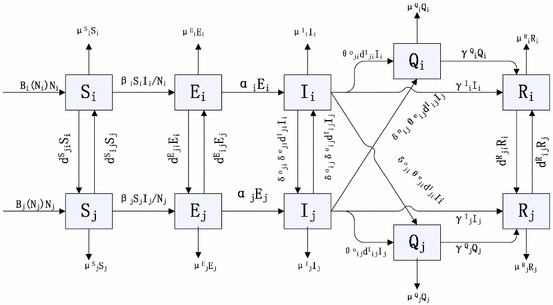
Flow chart of the disease transmission process between patch $i$ and patch $j$

As shown in Fig. 1, we neglect the transport-related infection and assume that individuals do not change their disease states when they travel from one patch to another; moreover, for the sake of focusing our study on the entry–exit screening, we ignore the contact tracing. Based on the above assumptions, our model can then be described by the following system

$$\begin{array}{c}\hfill \left\{\begin{array}{c}{\dot{S}}_i=B_i(N_i)N_i-\frac{{\mathit{\beta }}_i{S}_i{I}_i}{N_i}-{\mathit{\mu }}_i^S{S}_i-\sum _{j=1}^n{d}_{ji}^S{S}_i+\sum _{j=1}^n{d}_{ij}^S{S}_j,\hfill \\ {\dot{E}}_i=\frac{{\mathit{\beta }}_i{S}_i{I}_i}{N_i}-{\mathit{\alpha }}_i{E}_i-{\mathit{\mu }}_i^E{E}_i-\sum _{j=1}^n{d}_{ji}^E{E}_i+\sum _{j=1}^n{d}_{ij}^E{E}_j,\hfill \\ {\dot{I}}_i={\mathit{\alpha }}_i{E}_i-{\mathit{\gamma }}_i^I{I}_i-{\mathit{\mu }}_i^I{I}_i-\sum _{j=1}^n{d}_{ji}^I{I}_i+\sum _{j=1}^n{\mathit{\delta }}_{ij}^e{\mathit{\delta }}_{ij}^o{d}_{ij}^I{I}_j,\hfill \\ {\dot{Q}}_i=-{\mathit{\gamma }}_i^Q{Q}_i-{\mathit{\mu }}_i^Q{Q}_i+\sum _{j=1}^n{\mathit{\theta }}_{ji}^o{d}_{ji}^I{I}_i+\sum _{j=1}^n{\mathit{\theta }}_{ij}^e{\mathit{\delta }}_{ij}^o{d}_{ij}^I{I}_j,\hfill \\ {\dot{R}}_i={\mathit{\gamma }}_i^I{I}_i+{\mathit{\gamma }}_i^Q{Q}_i-{\mathit{\mu }}_i^R{R}_i-\sum _{j=1}^n{d}_{ji}^R{R}_i+\sum _{j=1}^n{d}_{ij}^R{R}_j,\hfill \\ i=1,2,\cdots ,n.\hfill \end{array}\right.\end{array}$$ 1

Throughout this paper, we use the following notation. For a vector $\mathbf{x}\in {\mathbb{R}}^n$, we use $\mathrm{diag}(\mathbf{x})$ to denote the $n\times n$ diagonal matrix, whose diagonal elements are the components of $\mathbf{x}$. We use the ordering in ${\mathbb{R}}^n$ generated by the cone ${\mathbb{R}}_{+}^n$, and that is, $\mathbf{x}\le \mathbf{y}$ if $\mathbf{y}-\mathbf{x}\in {\mathbb{R}}_{+}^n$, $\mathbf{x}<\mathbf{y}$ if $\mathbf{x}\le \mathbf{y}$ and $\mathbf{x}\ne \mathbf{y}$ and finally $\mathbf{x}\ll \mathbf{y}$ means $x_i<y_i$ for any index $i$. We use $(S(t),E(t),I(t),Q(t),R(t))$ to denote the vector

$$\begin{array}{cc}& (S_1(t),\cdots ,S_n(t),E_1(t),\cdots ,E_n(t),I_1(t),\cdots ,I_n(t),\hfill \\ \hfill & Q_1(t),\cdots ,Q_n(t),R_1(t),\cdots ,R_n{(t))}^T\in {\mathbb{R}}_{+}^{5n},\hfill \end{array}$$

and we denote $A_0=(S(0),E(0),I(0),Q(0),R(0)),$ then for any nonnegative initial condition $A_0$, it follows from the standard existence and uniqueness theorem for ordinary differential equations (Perko 2001) that system (1) admits a unique solution $(S(t),E(t),I(t),Q(t),R(t))$.

To show the existence of the disease-free equilibrium (DFE), we let $E_i=I_i=Q_i=R_i=0$, $i=1,2,\cdots ,n$ in (1) to get

$$\begin{array}{c}\hfill {\dot{S}}_i=B_i(S_i)S_i-\sum _{j=1}^n{d}_{ji}^S{S}_i+\sum _{j=1}^n{d}_{ij}^S{S}_j-{\mathit{\mu }}_i^S{S}_i,S_i(0)>0,i=1,2,\cdots ,n.\end{array}$$ 2

In order for system (2) to have a positive equilibrium, we assume that

(A4)

$s(\mathrm{diag}(B_i(0)-{\mathit{\mu }}_i^S)+D^S)>0$, where $s(·)$ represents the stability modulus of an $n\times n$ matrix and is defined by $s(M):=max\{\mathrm{Re}\mathit{\lambda }$, $\mathit{\lambda }$ is an eigenvalue of $M\}$.

Biologically, Assumption (A4) guarantees that the number of susceptible population is positive when there is no infective individual.

Following similar arguments as those in Wang and Zhao (2004), Zhao and Jing (1996), we have

Lemma 1

Under the assumptions (A1)–(A4), system (2) admits a unique positive equilibrium ${(S^0)}^T=(S_1^0,S_2^0,\cdots ,S_n^0)$, which is globally asymptotically stable for ${\mathbb{R}}_{+}^n\backslash \{0\}$.

Our preliminary results are the following two lemmas, whose proofs are similar to those given in Wang and Zhao (2004) and thus are omitted.

Lemma 2

Under the assumptions (A1)–(A4), system (1) admits a unique DFE $P^0=(S^0,\mathbf{0},\cdots ,\mathbf{0})$ with ${(S^0)}^T=(S_1^0,S_1^0,\cdots ,S_n^0)\in {\mathbb{R}}_{+}^n$ and ${\mathbf{0}}^T=(0,\cdots ,0)\in {\mathbb{R}}_{+}^n$.

Lemma 3

If (A1)–(A4) hold, then system (1) is dissipative, that is, there exists an $N^{\ast }>0$ such that every forward orbit $(S(t),E(t),I(t),Q(t),R(t))$ eventually enters the set $G:=\{(S(t),E(t),I(t),Q(t),R(t))\in {\mathbb{R}}_{+}^{5n}:{\sum }_{i=1}^n(S_i(t)+E_i(t)+I_i(t)+Q_i(t)+R_i(t))\le N^{\ast }\}$ and $G$ is positively invariant with respect to system (1).

Model Analysis

The Basic Reproduction Number

In this section, we identify the basic reproduction number, ${\mathfrak{R}}_0$ for system (1). Following the procedure introduced in van den Driessche and Watmough (2002), ${\mathfrak{R}}_0=\mathit{\rho }(F{V}^{-1})$, where $\mathit{\rho }$ represents the spectral radius of a matrix. Here $F=F_{3n\times 3n}$ and $V=V_{3n\times 3n}$ represent new infections and transition terms, respectively. They are given by

$$\begin{array}{c}\hfill F_{3n\times 3n}=\left(\begin{array}{ccc}0\hfill & F_{12}\hfill & 0\hfill \\ 0\hfill & 0\hfill & 0\hfill \\ 0\hfill & 0\hfill & 0\hfill \end{array}\right),V_{3n\times 3n}=\left(\begin{array}{ccc}{V}_{11}\hfill & 0\hfill & 0\hfill \\ V_{21}\hfill & V_{22}\hfill & 0\hfill \\ 0\hfill & V_{32}\hfill & V_{33}\hfill \end{array}\right)\end{array}$$

with

$$\begin{array}{cc}\hfill F_{12}=& \left(\begin{array}{cccc}{\mathit{\beta }}_1\hfill & 0\hfill & \dots \hfill & 0\hfill \\ 0\hfill & {\mathit{\beta }}_2\hfill & \dots \hfill & 0\hfill \\ ⋮\hfill & ⋮\hfill & \ddots \hfill & ⋮\hfill \\ 0\hfill & 0\hfill & \dots \hfill & {\mathit{\beta }}_n\hfill \end{array}\right)\hfill \\ \hfill V_{11}=& \left(\begin{array}{cccc}{\mathit{\alpha }}_1+{\mathit{\mu }}_1^E+\sum _{j=1}^n{d}_{j1}^E\hfill & -d_{12}^E\hfill & \dots \hfill & -d_{1n}^E\hfill \\ -d_{21}^E\hfill & {\mathit{\alpha }}_2+{\mathit{\mu }}_2^E+\sum _{j=1}^n{d}_{j2}^E\hfill & \dots \hfill & -d_{2n}^E\hfill \\ ⋮\hfill & ⋮\hfill & \ddots \hfill & ⋮\hfill \\ -d_{n1}^E\hfill & -d_{n2}^E\hfill & \dots \hfill & {\mathit{\alpha }}_n+{\mathit{\mu }}_n^E+\sum _{j=1}^n{d}_{jn}^E\hfill \end{array}\right)\hfill \\ \hfill V_{21}=& \left(\begin{array}{cccc}-{\mathit{\alpha }}_1\hfill & 0\hfill & \dots \hfill & 0\hfill \\ 0\hfill & -{\mathit{\alpha }}_2\hfill & \dots \hfill & 0\hfill \\ ⋮\hfill & ⋮\hfill & \ddots \hfill & ⋮\hfill \\ 0\hfill & 0\hfill & \dots \hfill & -{\mathit{\alpha }}_n\hfill \end{array}\right)\hfill \\ \hfill V_{22}=& \left(\begin{array}{cccc}{\mathit{\gamma }}_1^I+{\mathit{\mu }}_1^I+\sum _{j=1}^n{d}_{j1}^I\hfill & -{\mathit{\delta }}_{12}^e{\mathit{\delta }}_{12}^o{d}_{12}^I\hfill & \dots \hfill & -{\mathit{\delta }}_{1n}^e{\mathit{\delta }}_{1n}^o{d}_{1n}^I\hfill \\ -{\mathit{\delta }}_{21}^e{\mathit{\delta }}_{21}^o{d}_{21}^I\hfill & {\mathit{\gamma }}_2^I+{\mathit{\mu }}_2^I+\sum _{j=1}^n{d}_{j2}^I\hfill & \dots \hfill & -{\mathit{\delta }}_{2n}^e{\mathit{\delta }}_{2n}^o{d}_{2n}^I\hfill \\ ⋮\hfill & ⋮\hfill & \ddots \hfill & ⋮\hfill \\ -{\mathit{\delta }}_{n1}^e{\mathit{\delta }}_{n1}^o{d}_{n1}^I\hfill & -{\mathit{\delta }}_{n2}^e{\mathit{\delta }}_{n2}^o{d}_{n2}^I\hfill & \dots \hfill & {\mathit{\gamma }}_n^I+{\mathit{\mu }}_n^I+\sum _{j=1}^n{d}_{jn}^I\hfill \end{array}\right)\hfill \\ \hfill V_{32}=& \left(\begin{array}{cccc}-\sum _{j=1}^n{\mathit{\theta }}_{j1}^o{d}_{j1}^I\hfill & -{\mathit{\theta }}_{12}^e{\mathit{\delta }}_{12}^o{d}_{12}^I\hfill & \dots \hfill & -{\mathit{\theta }}_{1n}^e{\mathit{\delta }}_{1n}^o{d}_{1n}^I\hfill \\ -{\mathit{\theta }}_{21}^e{\mathit{\delta }}_{21}^o{d}_{21}^I\hfill & -\sum _{j=1}^n{\mathit{\theta }}_{j2}^o{d}_{j2}^I\hfill & \dots \hfill & -{\mathit{\theta }}_{2n}^e{\mathit{\delta }}_{2n}^o{d}_{2n}^I\hfill \\ ⋮\hfill & ⋮\hfill & \ddots \hfill & ⋮\hfill \\ -{\mathit{\theta }}_{n1}^e{\mathit{\delta }}_{n1}^o{d}_{n1}^I\hfill & -{\mathit{\theta }}_{n2}^e{\mathit{\delta }}_{n2}^o{d}_{n2}^I\hfill & \dots \hfill & -\sum _{j=1}^n{\mathit{\theta }}_{jn}^o{d}_{jn}^I\hfill \end{array}\right)\hfill \end{array}$$

and

$$\begin{array}{c}\hfill V_{33}=\left(\begin{array}{cccc}{\mathit{\gamma }}_1^Q+{\mathit{\mu }}_1^Q\hfill & 0\hfill & \dots \hfill & 0\hfill \\ 0\hfill & {\mathit{\gamma }}_2^Q+{\mathit{\mu }}_2^Q\hfill & \dots \hfill & 0\hfill \\ ⋮\hfill & ⋮\hfill & \ddots \hfill & ⋮\hfill \\ 0\hfill & 0\hfill & \dots \hfill & {\mathit{\gamma }}_n^Q+{\mathit{\mu }}_n^Q\hfill \end{array}\right)\end{array}$$

Both $V_{11}^{-1}$ and $V_{22}^{-1}$ are nonsingular $M$-matrices, which shows their inverses are nonnegative. This allows us to simplify the basic reproduction number as follows:

$$\begin{array}{c}\hfill {\mathfrak{R}}_0=\mathit{\rho }(F_{3n\times 3n}·V_{3n\times 3n}^{-1})=\mathit{\rho }(-F_{12}{V}_{22}^{-1}{V}_{21}{V}_{11}^{-1}).\end{array}$$ 3

Under some special circumstances, we have the following result.

Proposition 1

If ${\mathit{\alpha }}_i=\mathit{\alpha }$, ${\mathit{\gamma }}_i^I={\mathit{\gamma }}^I$, ${\mathit{\mu }}_i^E={\mathit{\mu }}^E$, ${\mathit{\mu }}_i^I={\mathit{\mu }}^I$, $d_{ij}^A=d$ for $A=E,I$, ${\mathit{\theta }}_{ij}^o={\mathit{\theta }}_{ij}^e=\mathit{\theta }\in [0,1]$, for $\forall i,j=1,2,\cdots ,n$ with $i\ne j$, then

$$\begin{array}{c}\hfill \underset{d\to 0^{+}}{lim}{\mathfrak{R}}_0=\underset{i}{max}\frac{\mathit{\alpha }{\mathit{\beta }}_i}{(\mathit{\alpha }+{\mathit{\mu }}^E)({\mathit{\gamma }}^I+{\mathit{\mu }}^I)}.\end{array}$$ 4

Proof

Note that in this special case,

$$\begin{array}{c}\hfill V_{11}=\left(\begin{array}{cccc}\mathit{\alpha }+{\mathit{\mu }}^E+(n-1)d\hfill & -d\hfill & \dots \hfill & -d\hfill \\ -d\hfill & \mathit{\alpha }+{\mathit{\mu }}^E+(n-1)d\hfill & \dots \hfill & -d\hfill \\ ⋮\hfill & ⋮\hfill & \ddots \hfill & ⋮\hfill \\ -d\hfill & -d\hfill & \dots \hfill & \mathit{\alpha }+{\mathit{\mu }}^E+(n-1)d\hfill \end{array}\right)\end{array}$$

and

$$\begin{array}{c}\hfill V_{22}=\left(\begin{array}{cccc}{\mathit{\gamma }}^I+{\mathit{\mu }}^I+(n-1)d\hfill & -{(1-\mathit{\theta })}^{2}d\hfill & \dots \hfill & -{(1-\mathit{\theta })}^{2}d\hfill \\ -{(1-\mathit{\theta })}^{2}d\hfill & {\mathit{\gamma }}^I+{\mathit{\mu }}^I+(n-1)\hfill & \dots \hfill & -{(1-\mathit{\theta })}^{2}d\hfill \\ ⋮\hfill & ⋮\hfill & \ddots \hfill & ⋮\hfill \\ -{(1-\mathit{\theta })}^{2}d\hfill & -{(1-\mathit{\theta })}^{2}d\hfill & \dots \hfill & {\mathit{\gamma }}^I+{\mathit{\mu }}^I+(n-1)d\hfill \end{array}\right)\end{array}$$

Thus, ${lim}_{d\to 0}{V}_{11}^{-1}=\frac{1}{\mathit{\alpha }+{\mathit{\mu }}^E}\mathrm{Id}$ and ${lim}_{d\to 0}{V}_{22}^{-1}=\frac{1}{{\mathit{\gamma }}^I+{\mathit{\mu }}^I}\mathrm{Id}$, where $\mathrm{Id}$ denotes the $n\times n$ identity matrix. Therefore, using (3), we obtain ${lim}_{d\to 0^{+}}{\mathfrak{R}}_0=\underset{i}{max}\frac{\mathit{\alpha }{\mathit{\beta }}_i}{(\mathit{\alpha }+{\mathit{\mu }}^E)(\mathit{\gamma }+{\mathit{\mu }}^I)}$. $\square$

Global Stability of the DFE

It follows from van den Driessche and Watmough (2002, Theorem 2) that the DFE is locally asymptotical stable if ${\mathfrak{R}}_0<1$ and is unstable if ${\mathfrak{R}}_0>1$.

Theorem 1

Assume that (A1)–(A4) are satisfied. If ${\mathfrak{R}}_0<1$, then the solution $(S(t),E(t),I(t),Q(t),R(t))$ of (1) satisfies

$$\begin{array}{c}\hfill \underset{t\to \infty }{lim}(S(t),E(t),I(t),Q(t),R(t))=P^0.\end{array}$$

Proof

By Lemma 3, there exists a $T^{\prime }>0$ and when $t>T^{\prime }$:

$$\begin{array}{c}\hfill \left\{\begin{array}{c}{\dot{E}}_i\le {\mathit{\beta }}_i{I}_i-{\mathit{\alpha }}_i{E}_i-{\mathit{\mu }}_i^E{E}_i-\sum _{j=1}^n{d}_{ji}^E{E}_i+\sum _{j=1}^n{d}_{ij}^E{E}_j,\hfill \\ {\dot{I}}_i={\mathit{\alpha }}_i{E}_i-{\mathit{\gamma }}_i^I{I}_i-{\mathit{\mu }}_i^I{I}_i-\sum _{j=1}^n{d}_{ji}^I{I}_i+\sum _{j=1}^n{\mathit{\delta }}_{ij}^e{\mathit{\delta }}_{ij}^o{d}_{ij}^I{I}_j,\hfill \\ {\dot{Q}}_i=-{\mathit{\gamma }}_i^Q{Q}_i-{\mathit{\mu }}_i^Q{Q}_i+\sum _{j=1}^n{\mathit{\theta }}_{ji}^o{d}_{ji}^I{I}_i+\sum _{j=1}^n{\mathit{\theta }}_{ij}^e{\mathit{\delta }}_{ij}^o{d}_{ij}^I{I}_j.\hfill \end{array}\right.\end{array}$$ 5

Set $M_1=F-V$ and ${\mathfrak{R}}_0<1$, it follows that $s(M_1)<0$. Let $v^T=(v_1,\dots ,v_n)$ be a positive eigenvector associated with $s(M_1)$. Choose $k>0$ small enough such that $kv\ll \mathit{\xi }$. Since $kv$ is a positive eigenvector associated with $s(M_1)$, the solution of the comparison system (5) is given by $kv{e}^{s(M_1)(t-T^{\prime })}$. According to the comparison principle (Smith 1995, 2008), $(E(t),I(t),Q(t))\le kv{e}^{s(M_1)(t-T^{\prime })}$, for $t>T^{\prime }$. Therefore, we get $(E(t),I(t),Q(t))\to (\mathbf{0},\mathbf{0},\mathbf{0})$ as $t\to \infty$. Further using the equations for $R_i$ of model (1), we can prove that ${lim}_{t\to \infty }R(t)=\mathbf{0}.$

Next we prove that $\underset{t\to \infty }{lim}S(t)=S^0$. Let $\mathit{\Phi }(t):{\mathbb{R}}_{+}^n\to {\mathbb{R}}_{+}^n$ be the solution semi-flow of (1), that is, $\mathit{\Phi }(t)(S_0,E_0,I_0,Q_0,R_0)=(S(t),E(t),I(t),Q(t),R(t))$ with the nonnegative initial value $(S_0,E_0,I_0,Q_0,R_0)$.

Given $(S_0,E_0,I_0,Q_0,R_0)\in G$ with $S_{i_0}\ne 0$, it easily follows that $S(t)\in \mathrm{Int}({\mathbb{R}}_{+}^n)$, $\forall t>0$. Let $\mathit{\omega }=\mathit{\omega }(S_0,E_0,I_0,Q_0,R_0)$ be the omega limit set of $\mathit{\Phi }(t)$. Since $(E(t),I(t),Q(t),$ $R(t))\to (\mathbf{0},\mathbf{0},\mathbf{0},\mathbf{0})$ as $t\to \infty$, there holds $\mathit{\omega }=\tilde{\mathit{\omega }}\times \{(\mathbf{0},\mathbf{0},\mathbf{0},\mathbf{0})\}$. We claim that there must be $\tilde{\mathit{\omega }}\ne \{\mathbf{0}\}$. Otherwise, if this is not true, i.e., $\tilde{\mathit{\omega }}=\{\mathbf{0}\}$, then we must have $\underset{t\to \infty }{lim}(S(t),E(t),I(t),Q(t),R(t))=(\mathbf{0},\mathbf{0},\mathbf{0},\mathbf{0},\mathbf{0})$. By Assumption $(\mathbf{A}\mathbf{4})$, we can choose a small $\mathit{\eta }>0$, such that $s(\mathrm{diag}(B_i(0)-{\mathit{\mu }}_i^S)+D^S-\mathit{\eta }\mathrm{diag}(11))>0$, where $11=(1,\dots ,1)$. It follows that there exists a $t_1>0$ such that $B_i(N_i(t))-\frac{{\mathit{\beta }}_i{I}_i(t)}{N_i(t)}\ge B_i(0+)-\mathit{\eta }$ for $\forall t\ge t_1,i=1,\dots ,n$. Then $S{(t)}^T=(S_1(t),S_2(t),\dots ,S_n(t))$ satisfies

$$\begin{array}{c}\hfill \begin{array}{c}{\dot{S}}_i(t)>(B_i(0+)-{\mathit{\eta }}_i)S_i(t)-\sum _{j=1}^n{d}_{ji}^S{S}_i(t)+\sum _{j=1}^n{d}_{ij}^S{S}_j(t)-{\mathit{\mu }}_i^S{S}_i(t).\hfill \end{array}\end{array}$$ 6

Let ${\mathit{\omega }}^T=({\mathit{\omega }}_1,\dots ,{\mathit{\omega }}_n)$ be a positive eigenvector of the matrix $\mathrm{diag}(B_i(0)-{\mathit{\mu }}_i^S)+D^S-\mathit{\eta }\mathrm{diag}(11)$ associated with the eigenvalue $s(\mathrm{diag}(B_i(0)-{\mathit{\mu }}_i^S)+D^S-\mathit{\eta }\mathrm{diag}(11))$. Choose a small number $\mathit{\alpha }>0$ such that $S(t_1)>\mathit{\alpha }\mathit{\omega }$. Then the comparison principle (Smith 1995, 2008) implies that

$$\begin{array}{c}\hfill S(t)\ge \mathit{\alpha }\mathit{\omega }{e}^{{\displaystyle s(\mathrm{diag}(B_i(0)-{\mathit{\mu }}_i^S)+D^S-\mathit{\eta }\mathrm{diag}(11))(t-t_1)}},\forall t\ge t_1\end{array}$$

and then $S_i(t)\to \infty ,i=1,2\dots n$, a contradiction. It is easy to see that ${\mathit{\Phi }}_1(t){|}_{\mathit{\omega }}(S(t)$, $\mathbf{0},\mathbf{0},\mathbf{0},\mathbf{0})=({\mathit{\Phi }}_1(t)S(t),\mathbf{0},\mathbf{0},\mathbf{0},\mathbf{0})$, where ${\mathit{\Phi }}_1(t)$ is the solution semi-flow of system (2). By Hirsch et al. (2001, Lemma 2.10), $\mathit{\omega }$ is an internal chain transitive set for $\mathit{\Phi }(t)$, and hence, ${\mathit{\omega }}_1$ is an internal chain transitive set for ${\mathit{\Phi }}_1(t)$. Since ${\mathit{\omega }}_1\ne 0$ and $S^0$ is globally asymptotically stable for (1) in ${\mathbb{R}}_{+}^n\backslash \{0\}$, we have ${\mathit{\omega }}_1\cap W^s(S^0)\ne \mathrm{\varnothing }$. By (Hirsch et al. 2001, Theorem 3.1 and Remark 4.6), we then get ${\mathit{\omega }}_1=S^0$, proving $\mathit{\omega }=\{P^0\}$. This proves Theorem 1. $\square$

Disease Persistence and Existence of the Endemic Equilibrium

It follows from van den Driessche and Watmough (2002, Theorem 2) that the DFE $P^0$ is unstable if ${\mathfrak{R}}_0>1$. The following result shows that ${\mathfrak{R}}_0>1$ actually implies that model (1) admits at least one endemic equilibrium (EE) and the disease persists uniformly.

Define $X=\{(S,E,I,Q,R):S_i\ge 0,E_i\ge 0,I_i\ge 0,Q_i\ge 0,R_i\ge 0,i=1,2,\dots ,n$}, $X_0=\{(S,E,I,Q,R):E_i>0,I_i>0,i=1,2,\dots ,n\}$, $\mathit{\partial }{X}_0=X\backslash X_0$.

Theorem 2

Suppose the assumptions (A1)–(A4) hold and the basic reproduction number ${\mathfrak{R}}_0>1$. Then system (1) is uniformly persistent, that is, there exists a positive constant $\mathit{ϵ}>0$ such that every solution $A(t)$ of (1) with

$$\begin{array}{c}\hfill A_0\in {\mathbb{R}}_{+}^n\times ({\mathbb{R}}_{+}^n\backslash \{0\})\times ({\mathbb{R}}_{+}^n\backslash \{0\})\times {\mathbb{R}}_{+}^n\times {\mathbb{R}}_{+}^n\end{array}$$

satisfies

$$\begin{array}{c}\hfill \underset{t\to \infty }{lim}inf(E_i(t),I_i(t))\ge (\mathit{ϵ},\mathit{ϵ}),i=1,\cdots ,n.\end{array}$$

Moreover, there exists at least one EE.

Proof

Let $\mathit{\Phi }(t):X\to X$ be the solution flow associated with system (1), that is, $\mathit{\Phi }(t)(A_0)=A(t)$.

It follows from Lemma 3 that $X$ is positively invariant and system (1) is point dissipative. By the comparison principle for cooperative systems (Smith 1995, 2008), it follows that $(E,I)\gg (\mathbf{0},\mathbf{0})$. This implies that $X_0$ is positively invariant, thus $\mathit{\partial }{X}_0$ is relatively closed in $X$.

Set $M_{\mathit{\partial }}=\{A_0\in X:A(t)\in \mathit{\partial }{X}_0,\forall t\ge 0\}$. We claim that

$$\begin{array}{c}\hfill M_{\mathit{\partial }}=\{(E(t),I(t))=(\mathbf{0},\mathbf{0}),\forall t\ge 0\}.\end{array}$$

Suppose on the contrary, i.e., there exists a $t_0\ge 0$ such that $E(t_0)>\mathbf{0}$, or $I(t_0)>\mathbf{0}$. Without loss of generality, we assume that $E(t_0)>\mathbf{0}$. We partition $\{1,2,\dots ,n\}$ into two sets, $Z_1$ and $Z_2$, such that

$$\begin{array}{c}\hfill E_i(t_0)=0,\forall i\in Z_1,\text{and}{E}_i(t_0)>0,\forall i\in Z_2.\end{array}$$

Next we claim that $E_i(t)>0$ for $t_0<t<t_0+{\mathit{ϵ}}_0,\forall i=1,\cdots ,n$ for ${\mathit{ϵ}}_0>0$ small enough, which could be easily verified provided that $Z_1=\mathrm{\varnothing }$. Assume $Z_1\ne \mathrm{\varnothing }$, since $Z_2\ne \mathrm{\varnothing }$ as $E(t_0)>\mathbf{0}$. Then for $\forall i\in Z_1$,

$$\begin{array}{c}\hfill \begin{array}{cc}{\dot{E}}_i(t_0)\hfill & =\frac{{\mathit{\beta }}_i{S}_i(t_0)I_i(t_0)}{N_i(t_0)}-{\mathit{\alpha }}_i{E}_i(t_0)-\sum _{j=1}^n{d}_{ji}^E{E}_i(t_0)+\sum _{j=1}^n{d}_{ij}^E{E}_j(t_0)-{\mathit{\mu }}_i^E{E}_i(t_0)\hfill \\ \hfill & =\frac{{\mathit{\beta }}_i{S}_i(t_0)I_i(t_0)}{N_i(t_0)}+\sum _{j\in Z_2}{d}_{ij}^E{E}_j(t_0).\hfill \end{array}\end{array}$$

According to the irreducibility of $D^E$, there is always a chain $j_1,j_2,\dots ,j_n$ with $j_1=j,j_n=i$, which ensures that ${\sum }_{j\in Z_2}{d}_{ij}^E{E}_j(t_0)>0\Rightarrow {\dot{E}}_i(t_0)>0$, and hence, there exists an ${\mathit{ϵ}}_0>0$ such that $E_i(t)>0$ for $t_0<t<t_0+{\mathit{ϵ}}_0$. Clearly, we can restrict ${\mathit{ϵ}}_0>0$ small enough such that $E_i(t)>0,t_0<t<t_0+{\mathit{ϵ}}_0$ for $\forall i\in Z_1\cup Z_2$. This proves $E_i(t)>0,i=1,\dots ,n,t_0<t<t_0+{\mathit{ϵ}}_0$.

Using the equation of system (1) for $I_i$, we obtain that either $I_i(t_0)>0$, or $I_i(t_0)=0$ and ${\dot{I}}_i(t_0)>0$ holds true, for both cases, we have $I_i(t)>0,t_0<t<t_0+{\mathit{ϵ}}_1,\forall i=1,\cdots ,n$ for ${\mathit{ϵ}}_1>0$ sufficiently small. This results in $A(t)\notin \mathit{\partial }{X}_0$ for $t_0<t<t_0+min\{{\mathit{ϵ}}_0,{\mathit{ϵ}}_1\}$, which contradicts the assumption of $M_{\mathit{\partial }}$, this proves $E(t)=\mathbf{0},\forall t\ge 0$. Repeating the same way on $I(t)$, we can show that $I(t)=\mathbf{0}\forall t\ge 0$, and thus we verify the above claim on $M_{\mathit{\partial }}$.

Next we show that the solution $A(t)$ through $A_0\in X_0$ satisfies

$$\begin{array}{c}\hfill \underset{t\to \infty }{lim\; sup}\underset{1\le i\le n}{max}\{E_i(t),I_i(t)\}>{\mathit{ϵ}}_2.\end{array}$$

for some positive constant ${\mathit{ϵ}}_2$.

Suppose this is not true, there must exist a $T_1>0$ such that

$$\begin{array}{c}\hfill 0<\underset{1\le i\le n}{max}\{E_i(t),I_i(t)\}\le {\mathit{ϵ}}_2,\text{for}\text{all}t\ge T_1,\end{array}$$

then it follows from the equations of $Q_i,R_i,i=1,\dots ,n$ of system (1) that $\exists k_0>0$, such that $(Q_i(t),R_i(t))<(k_0{\mathit{ϵ}}_2,k_0{\mathit{ϵ}}_2)$. As the boundedness of $S$, we can restrict $\frac{{\mathit{\beta }}_i{S}_i{I}_i}{N_i}\le \mathit{\xi }({\mathit{ϵ}}_2)$. Then we have

$$\begin{array}{cc}\hfill {\dot{S}}_i=& B_i(N_i)N_i-\frac{{\mathit{\beta }}_i{S}_i{I}_i}{N_i}-\sum _{j=1}^n{d}_{ji}^S{S}_i+\sum _{j=1}^n{d}_{ij}^S{S}_j-{\mathit{\mu }}_i^S{S}_i\hfill \\ \hfill \ge & B_i(S_i+(2k_0+2){\mathit{ϵ}}_2)S_i-({\mathit{\mu }}_i^S+\mathit{\xi }({\mathit{ϵ}}_2))S_i-\sum _{j=1}^n{d}_{ji}{S}_i+\sum _{j=1}^n{d}_{ij}{S}_j\hfill \end{array}$$

Consider the following auxiliary equation

$$\begin{array}{cc}\hfill {\dot{\underset{\_}{S}}}_i=& B_i({\underset{\_}{S}}_i+(2k_0+2){\mathit{ϵ}}_2){\underset{\_}{S}}_i-({\mathit{\mu }}_i^S+\mathit{\xi }({\mathit{ϵ}}_2)){\underset{\_}{S}}_i-\sum _{j=1}^n{d}_{ji}^S{\underset{\_}{S}}_i+\sum _{j=1}^n{d}_{ij}^S{\underset{\_}{S}}_j,\hfill \\ \hfill & ({\underset{\_}{S}}_1(T_1),\dots ,{\underset{\_}{S}}_n(T_1))=(S_1(T_1),\dots ,S_n(T_1)),i=1,\dots ,n.\hfill \end{array}$$ 7

By the comparison principle Smith (1995), Smith (2008), we have $S(t)\ge \underset{\_}{S}(t),\forall t\ge T_1$, here ${\underset{\_}{S}}^T(t)=({\underset{\_}{S}}_1(t),\dots ,{\underset{\_}{S}}_n(t)).$ By (7), there exists a constant vector $S^0({\mathit{ϵ}}_2)>\mathbf{0}$ such that ${(S^0)}^T({\mathit{ϵ}}_2)$ is globally asymptotically stable for (7) and that $S^0(0)=S^0$. Then there exists a sufficiently small $\mathit{\eta }$ with ${\mathit{\eta }}^T=({\mathit{\eta }}_1,\dots ,{\mathit{\eta }}_n)\in {\mathbb{R}}_{+}^n$ and a sufficiently large $T>0$, such that $S^0({\mathit{ϵ}}_2)>S^0-\mathit{\eta }$, and that $S(t)\ge S^0({\mathit{ϵ}}_2)\ge S^0-\mathit{\eta }$ for all $t\ge T+T_1$. As a consequence, $\frac{S_i}{N_i}=1-\frac{E_i+I_i+Q_i+R_i}{N_i}\ge 1-\frac{(2k_0+2){\mathit{ϵ}}_2}{S_i^0-{\mathit{\eta }}_i},\forall t\ge T+T_1$, hence we have

$$\begin{array}{cc}\hfill {\dot{E}}_i=& \frac{{\mathit{\beta }}_i{S}_i{I}_i}{N_i}-{\mathit{\alpha }}_i{E}_i-\sum _{j=1}^n{d}_{ji}^E{E}_i+\sum _{j=1}^n{d}_{ij}^E{E}_j-{\mathit{\mu }}_i^E{E}_i\hfill \\ \hfill \ge & {\mathit{\beta }}_i{I}_i(1-\frac{(2k_0+2){\mathit{ϵ}}_2}{S_i^0-{\mathit{\eta }}_i})-({\mathit{\alpha }}_i+{\mathit{\mu }}_i^E)E_i-\sum _{j=1}^n{d}_{ji}^E{E}_i+\sum _{j=1}^n{d}_{ij}^E{E}_j.\hfill \end{array}$$

Consider the following auxiliary system:

$$\begin{array}{c}\hfill \left\{\begin{array}{c}\dot{{\tilde{E}}_i}={\mathit{\beta }}_i{\tilde{I}}_i(1-\frac{(2k_0+2){\mathit{ϵ}}_2}{S_i^0-{\mathit{\eta }}_i})-{\mathit{\alpha }}_i{\tilde{E}}_i-{\mathit{\mu }}_i^E{\tilde{E}}_i-\sum _{j=1}^n{d}_{ji}^E{\tilde{E}}_i+\sum _{j=1}^n{d}_{ij}^E{\tilde{E}}_j,\hfill \\ \dot{{\tilde{I}}_i}={\mathit{\alpha }}_i{\tilde{E}}_i-{\mathit{\gamma }}_i{\tilde{I}}_i-{\mathit{\mu }}_i^I{\tilde{I}}_i-\sum _{j=1}^n{d}_{ji}^I{\tilde{I}}_i+\sum _{j=1}^n{\mathit{\delta }}_{ij}^e{\mathit{\delta }}_{ij}^o{d}_{ij}^I{\tilde{I}}_j,\hfill \\ \dot{{\tilde{Q}}_i}=-{\mathit{\gamma }}_i{\tilde{Q}}_i-{\mathit{\mu }}_i^I{\tilde{Q}}_i+\sum _{j=1}^n{\mathit{\theta }}_{ji}^o{d}_{ji}^Q{\tilde{I}}_i+\sum _{j=1}^n{\mathit{\theta }}_{ij}^e{\mathit{\delta }}_{ij}^o{d}_{ij}^Q{\tilde{I}}_j.\hfill \end{array}\right.\end{array}$$ 8

Since ${\mathfrak{R}}_0>1$, we know that the matrix $(1-\frac{(2k_0+2){\mathit{ϵ}}_2}{S_i^0-{\mathit{\eta }}_i})M_1$ has a positive eigenvalue $s((1-\frac{(2k_0+2){\mathit{ϵ}}_2}{S_i^0-{\mathit{\eta }}_i})M_1)$ with a positive eigenvector. Let ${\tilde{v}}^T=(v_1,\dots ,v_n)$ be a positive eigenvector associated with $s((1-\frac{(2k_0+2){\mathit{ϵ}}_2}{S_i^0-{\mathit{\eta }}_i})M_1)$, then the solution of Eq. (8) is given by $k_1\tilde{v}{e}^{s((1-\frac{(2k_0+2){\mathit{ϵ}}_2}{S_i^0-{\mathit{\eta }}_i})M_1)}$. Again, by the comparison principle (Smith 1995, 2008), we have

$$\begin{array}{c}\hfill (E(t),I(t),Q(t))\ge k_1\tilde{v}{e}^{s((1-\frac{(2k_0+2){\mathit{ϵ}}_2}{S_i^0-{\mathit{\eta }}_i})M_1)t},\forall t\ge T.\end{array}$$

Then $(E_i(t),I_i(t),Q_i(t))\to (\infty ,\infty ,\infty ),i=1,2,\dots ,n$, for $t\to \infty$, which leads to a contradiction.

Note that ${(S^0)}^T$ is globally asymptotically stable in ${\mathbb{R}}_{+}^n\backslash \{0\}$ for system (2). By the afore-mentioned claim, it then follows that $(\mathbf{0},\mathbf{0},\mathbf{0},\mathbf{0},\mathbf{0})$ and $P_0$ are isolated invariant sets in $X$, $W^s((\mathbf{0},\mathbf{0},\mathbf{0},\mathbf{0},\mathbf{0}))\cap X_0=\mathrm{\varnothing }$, and $W^s(P_0)\cap X_0=\mathrm{\varnothing }$. Clearly, every orbit in $M_{\mathit{\partial }}$ converges to either $(\mathbf{0},\mathbf{0},\mathbf{0},\mathbf{0},\mathbf{0})$ or $P_0$, and $(\mathbf{0},\mathbf{0},\mathbf{0},\mathbf{0},\mathbf{0})$ and $P_0$ are acyclic in $M_{\mathit{\partial }}$. By Hirsch et al. (2001, Theorem 4.3 and Remark 4.3), we conclude that system (1) is uniformly persistent with respect to $(X_0,\mathit{\partial }{X}_0)$. By Zhao (1995, Theorem 2.4), system (1) has at least one equilibrium $(S^{\ast },E^{\ast },I^{\ast },Q^{\ast },R^{\ast })\in X_0$, with $E^{\ast }\gg \mathbf{0}$ and $I^{\ast }\gg \mathbf{0}$. We further show that $S^{\ast }\in {\mathbb{R}}_{+}^n\backslash \{\mathbf{0}\}$. Suppose $S^{\ast }=\mathbf{0}$, by the sum of equations of $E_i$ in (1), we get $0=\sum _{i=1}^n({\mathit{\alpha }}_i+{\mathit{\mu }}_i)E_i^{\ast }$, and hence $E^{\ast }=\mathbf{0}$, a contradiction. Thus the proof is complete. 2. $\square$

Case Study for the 2009 Influenza A (H1N1)

In this section, we use numerical simulations to explore the impacts of various screening strategies on the control of 2009 influenza A (H1N1) pandemic.

Sensitivity Analysis of ${\mathfrak{R}}_0$ on Parameters for a Two-Patch Model

We consider a special case of system (1) with $n=2$ as follows:

$$\begin{array}{c}\hfill \left\{\begin{array}{c}{\displaystyle {\dot{S}}_1=B_1(N_1)N_1-\frac{{\mathit{\beta }}_1{S}_1{I}_1}{N_1}-{\mathit{\mu }}_1^S{S}_1-d_{21}^S{S}_1+d_{12}^S{S}_2,}\hfill \\ {\displaystyle {\dot{E}}_1=\frac{{\mathit{\beta }}_1{S}_1{I}_1}{N_1}-{\mathit{\alpha }}_1{E}_1-{\mathit{\mu }}_1^E{E}_1-d_{21}^E{E}_1+d_{12}^E{E}_2,}\hfill \\ {\displaystyle {\dot{I}}_1={\mathit{\alpha }}_1{E}_1-{\mathit{\gamma }}_1^I{I}_1-{\mathit{\mu }}_1^I{I}_1-d_{21}^I{I}_1+{\mathit{\delta }}_{12}^e{\mathit{\delta }}_{12}^o{d}_{12}^I{I}_2,}\hfill \\ {\displaystyle {\dot{Q}}_1=-{\mathit{\gamma }}_1^Q{Q}_1-{\mathit{\mu }}_1^Q{Q}_1+{\mathit{\theta }}_{21}^o{d}_{21}^I{I}_1+{\mathit{\theta }}_{12}^e{\mathit{\delta }}_{12}^o{d}_{12}^I{I}_2,}\hfill \\ {\displaystyle {\dot{R}}_1={\mathit{\gamma }}_1^I{I}_1+{\mathit{\gamma }}_1^Q{Q}_1-{\mathit{\mu }}_1^R{R}_1-d_{21}^R{R}_1+d_{12}^R{R}_2,}\hfill \\ {\displaystyle {\dot{S}}_2=B_2(N_2)N_2-\frac{{\mathit{\beta }}_2{S}_2{I}_2}{N_2}-{\mathit{\mu }}_2^S{S}_2-d_{12}^S{S}_2+d_{21}^S{S}_1,}\hfill \\ {\displaystyle {\dot{E}}_2=\frac{{\mathit{\beta }}_2{S}_2{I}_2}{N_2}-{\mathit{\alpha }}_2{E}_2-{\mathit{\mu }}_2^E{E}_2-d_{12}^E{E}_2+d_{21}^E{E}_1,}\hfill \\ {\displaystyle {\dot{I}}_2={\mathit{\alpha }}_2{E}_2-{\mathit{\gamma }}_2^I{I}_2-{\mathit{\mu }}_2^I{I}_2-d_{22}^I{I}_2+{\mathit{\delta }}_{21}^e{\mathit{\delta }}_{21}^o{d}_{21}^I{I}_1,}\hfill \\ {\displaystyle {\dot{Q}}_2=-{\mathit{\gamma }}_2^Q{Q}_2-{\mathit{\mu }}_2^I{Q}_2+{\mathit{\theta }}_{12}^o{d}_{12}^I{I}_2+{\mathit{\theta }}_{21}^e{\mathit{\delta }}_{21}^o{d}_{21}^I{I}_1,}\hfill \\ {\displaystyle {\dot{R}}_2={\mathit{\gamma }}_2^I{I}_2+{\mathit{\gamma }}_2^Q{Q}_2-{\mathit{\mu }}_2^R{R}_2-d_{12}^R{R}_2+d_{21}^R{R}_1.}\hfill \end{array}\right.\end{array}$$ 9

The basic reproduction number of system (9) is given by

$$\begin{array}{c}\hfill {\mathfrak{R}}_0\left|{}_{(9)}\right.=\mathit{\rho }\left(-{\tilde{F}}_{12}{\tilde{V}}_{22}^{-1}{\tilde{V}}_{21}{\tilde{V}}_{11}^{-1}\right)\end{array}$$ 10

where

$$\begin{array}{cc}\hfill {\tilde{F}}_{12}=& \left(\begin{array}{cc}{\mathit{\beta }}_1& 0\\ 0& {\mathit{\beta }}_2\end{array}\right);{\tilde{V}}_{21}=\left(\begin{array}{cc}{\mathit{\gamma }}_1^I+{\mathit{\mu }}_1^I+d_{21}^I& -{\mathit{\delta }}_{12}^e{\mathit{\delta }}_{12}^o{d}_{12}^I\\ -{\mathit{\delta }}_{21}^e{\mathit{\delta }}_{21}^o{d}_{21}^I& {\mathit{\gamma }}_2^I+{\mathit{\mu }}_2^I+d_{12}^I\end{array}\right);\hfill \\ \hfill {\tilde{V}}_{21}=& \left(\begin{array}{cc}-{\mathit{\alpha }}_1& 0\\ 0& -{\mathit{\alpha }}_2\end{array}\right);{\tilde{V}}_{11}=\left(\begin{array}{cc}{\mathit{\alpha }}_1+{\mathit{\mu }}_1^E+d_{21}^E& -d_{12}^E\\ -d_{21}^E& {\mathit{\alpha }}_2+{\mathit{\mu }}_2^E+d_{12}^E\end{array}\right).\hfill \end{array}$$

Note that the basic reproduction number ${\mathfrak{R}}_0$ defined in (10) involves a group of parameters. To identify to which parameters ${\mathfrak{R}}_0$ is sensitive, we carry out a sensitivity analysis by evaluating the partial rank correlation coefficients (PRCCs) for all input parameters against the output variable ${\mathfrak{R}}_0$ (Blower and Dowlatabadi 1994; Wu et al. 2013). We take parameter values as in Table 1. Moreover, we denote $\mathit{\beta }={\mathit{\beta }}_1={\mathit{\beta }}_2,\mathit{\alpha }={\mathit{\alpha }}_1={\mathit{\alpha }}_2$, ${\mathit{\mu }}^K={\mathit{\mu }}_1^K={\mathit{\mu }}_2^K;d^K=d_{12}^K=d_{21}^K,(K=S,I,E,R)$, and we set $\mathit{\gamma }=1/6.56={\mathit{\gamma }}_1^I={\mathit{\gamma }}_2^I$, $d^I=0.5\times d^S,d^E=0.9\times d^S$, where $d^S=0.135$; we also assume ${\mathit{\theta }}^e=0.37={\mathit{\theta }}_{21}^e={\mathit{\theta }}_{12}^e,{\mathit{\theta }}^o={\mathit{\theta }}_{21}^o={\mathit{\theta }}_{12}^o$ with ${\mathit{\theta }}^o=0.3\times {\mathit{\theta }}^e$.

Table 1.

The parameter estimates for the 2009 influenza A (H1N1) pandemic

Parameters $i,j=1,2$ $i\ne j$	Definitions	Values	References
${\mathit{\beta }}_i$	The infection rate (days${}^{-1}$) in patch $i$	0.3936	Tang et al. (2012)
${\mathit{\alpha }}_i$	Rate of progression to latent (days${}^{-1}$) in patch $i$	$0.55$	Tang et al. (2012)
${\mathit{\gamma }}_i^I$	Recovery rate (days${}^{-1}$) in patch $i$	1/7.48–1/6	Tang et al. (2012), Xiao et al. (2015)
${\mathit{\mu }}_i^S$	The natural death rate (days${}^{-1}$) in patch $i$	$3.805\times {10}^{-5}$	Wang and Wang (2012)
${\mathit{\mu }}_i^I,({\mathit{\mu }}_i^E)$	Infectious (Exposed) death rate (days${}^{-1}$) in patch $i$	$5.307\times {10}^{-5}$	Xu et al. (2011)
${\mathit{\theta }}_{ij}^e$	Entry screening rate of travelers from patch $j$ to $i$	0.33–0.4556	Cowling et al. (2010), Li et al. (2013)
${\mathit{\theta }}_{ij}^o$	Exit screening rate of travelers from patch $j$ to $i$	0.165–0.2228	Estimated
$d_{ij}^S,(d_{ij}^R)$	Dispersal rate (days${}^{-1}$) of the susceptible (recovered) from patch $j$ to $i$	0.0135–0.135	Tang et al. (2010)
$d_{ij}^I,(d_{ij}^E)$	Dispersal rate (days${}^{-1}$) of the infectious (exposed) from patch $j$ to $i$	0.0122–0.122	Estimated

We show that the infection rate $\mathit{\beta }$ is the most sensitive parameter of ${\mathfrak{R}}_0$ of system (9). For other coefficients, Fig. 2 shows that the six parameters with most impacts on ${\mathfrak{R}}_0$ are the rate of progression to latent ($\mathit{\alpha }$), the recovery rate ($\mathit{\gamma }$), the entry screening rate (${\mathit{\theta }}^e$), the exit screening rate (${\mathit{\theta }}^o$), the susceptible dispersal rate ($d^S$), and the infected dispersal rate ($d^I$).

Fig. 2.

Partial rank correlation coefficients illustrating the dependence of ${\mathfrak{R}}_0$ on each parameter

Impacts of Various Screening Strategies

For the model (1), if patch $i$ is not connected to any other patch, then the patch-specific basic reproduction number is given by

$$\begin{array}{c}\hfill {\mathfrak{R}}_{0i}=\frac{{\mathit{\beta }}_i{\mathit{\alpha }}_i}{({\mathit{\alpha }}_i+{\mathit{\mu }}_i^E)({\mathit{\gamma }}_i^I+{\mathit{\mu }}_i^I)}.\end{array}$$

If ${\mathfrak{R}}_{0i}<1$, then we call patch $i$ a low-risk patch, while if ${\mathfrak{R}}_{0i}>1$, then we call it a high-risk patch (Allen et al. 2007). Therefore, the disease persists in isolated high-risk patches and dies out in isolated low-risk patches. During the 2009 H1N1 pandemic, Mexico could be regarded as a high-risk patch, and it is believed that the pandemic was caused by the global connection with Mexico (Khan et al. 2013; Smith et al. 2009).

To examine the impacts of various screening strategies on the control of diseases, we assume there are one high-risk patch, labeled as patch $1$, and $4$ low-risk patches, labeled as patches $2,3,4$, and $5$, and the overall basic reproduction number ${\mathfrak{R}}_0$ is larger than $1$.

For simulation purpose, we take parameter values as in Table 1: ${\mathit{\mu }}_i^S={\mathit{\mu }}_i^R=3.805\times {10}^{-5}$, ${\mathit{\mu }}_i^E={\mathit{\mu }}_i^I=5.307\times {10}^{-5},{\mathit{\alpha }}_i=0.55$ for $i=1,\cdots ,5$, and ${\mathit{\beta }}_1=0.3936\gg {\mathit{\beta }}_i=0.15$, ${\mathit{\gamma }}_1^I=1/7.48<{\mathit{\gamma }}_i^I=1/6$ for $i=2,\cdots ,5$. For this set of parameter values, ${\mathfrak{R}}_{01}=2.772\gg 1$, ${\mathfrak{R}}_{02}={\mathfrak{R}}_{03}={\mathfrak{R}}_{04}={\mathfrak{R}}_{05}=0.900<1$. That is, patch $1$ is a high-risk patch, and the remaining $4$ patches are low-risk patches. Considering reduced dispersal rates for exposed and infectious individuals, we take $d_{ij}^E=0.9\times d_{ij}^S,d_{ij}^I=0.5\times d_{ij}^S,i\ne j.$ Further we assume that patch $5$ has less communication with patch $1$. For simplicity, we assume $d_{15}^S=d_{51}^S=0.1\times d^S$, $d_{1j}^S=d_{j1}^S=d^S$ for $j=2,3,4$ and $d_{ij}^S=d_{ji}^S=d^S$ for $i,j=2,3,4,5$ and $i\ne j$.

The question we want to address is: what types of screening strategies are capable of preventing the endemic disease? To answer this question, we explore the outcomes of several possible screening strategies.

We first consider Strategy I, “indiscriminate entry–exit screening” strategy: regardless of the risk level and dispersal rates, same strength of entry and exit screenings are implemented to each patch. That is, ${\mathit{\theta }}_{ij}^o={\mathit{\theta }}_{ij}^e=\mathit{\theta }$ for $i,j=1,\cdots ,5$. For the parameter values taken, we find numerically that this strategy is the most effective of the six strategies considered. Moreover, the detection rate needs to be higher as the dispersal rates decrease, and when the dispersal rate $d^S<d_{c1}=0.090$, the screening strategy cannot control the disease even when the detection is perfect (see Fig. 3a).

Fig. 3.

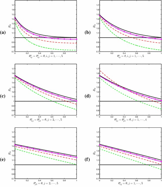
Plots of ${\mathfrak{R}}_0$ under screening Strategies I–VI. Parameters: ${\mathit{\gamma }}_1^I=1/7.48;{\mathit{\gamma }}_2^I={\mathit{\gamma }}_3^I={\mathit{\gamma }}_4^I={\mathit{\gamma }}_4=1/6,{\mathit{\beta }}_1=0.3936;{\mathit{\beta }}_2={\mathit{\beta }}_3={\mathit{\beta }}_4={\mathit{\beta }}_5=0.15.$ The black solid line: $d^S=0.09$; The pink solid line with $\ast$: $d^S=0.095$; the blue dotted line: $d^S=0.097$; the red dot-and-dash line $d^S=0.107$; the green dashed line: $d^S=0.135$ (Color figure online)

Strategy II is called the “indiscriminate entry screening” strategy: only entry screening of each patch is implemented. That is, ${\mathit{\theta }}_{ij}^e=\mathit{\theta }$ for $i,j=1,...,5$. By comparing Fig. 3a with Fig. 3b, we find that Strategy II can control the disease if Strategy I can, but Strategy II requires higher successful detection rate of infectious travelers.

Strategy III in consideration is called the “targeted entry screening”: only apply entry screening for travel from and to the high-risk patch, patch $1$. That is, ${\mathit{\theta }}_{j1}^e={\mathit{\theta }}_{1j}^e=\mathit{\theta }$ for $j=2,3,4,5$. As shown in Fig. 3c, the disease will die out if the dispersal rate $d^S$ is higher than a critical value $d_{c2}$ (in our simulation, $d_{c2}=0.095$).

In practice, a natural question to be asked is: do we need to implement screening in all patches? To answer this question, we examine Strategy IV, “selective entry screening”: only apply entry screening to the high-risk patch and patches that are highly connected to the high-risk patch (i.e., those patches with larger dispersal rates). In our simulation, we assume ${\mathit{\theta }}_{j1}^e={\mathit{\theta }}_{1j}^e=\mathit{\theta },j=2,3,4$. Figure 3d indicates that this strategy can also eliminate the disease if the dispersal rate $d^S$ is higher than the critical value $d_{c3}=0.097$. This implies that there is no need to implement screening at all patches.

It is worth mentioning Strategy V, “one-way entry screening”: applying entry screening at low-risk patches to individuals traveling from the high-risk patch only. In our simulations, we take ${\mathit{\theta }}_{j1}^e=\mathit{\theta }$ for $j=2,3,4,5$, and all other screening rates are set to be zero. Then for our chosen parameter values, the dispersal rate $d^S$ must be sufficiently large, larger than $d_{c4}=0.135$ in our simulations (See Fig. 3e). However, another “one-way entry screening”, Strategy VI: applying entry screening at the high-risk patch to travelers from all low-risk patches is capable of eradicating the disease. In our simulation, we choose ${\mathit{\theta }}_{1j}^e=\mathit{\theta }$ for $j=2,3,4,5$, and we can lower ${\mathfrak{R}}_0$ to be less than $1$ provided that $d^S>d_{c5}=0.107$ (see Fig.  3f).

Summary and Discussion

In this paper, we have investigated a general multi-patch SEIQR model with entry–exit screenings. Our theoretical results, Theorems 1 and 2, were established by appealing to the comparison principle and uniform persistence principle. Our results show that the disease dies out when ${\mathfrak{R}}_0<1$ and persists when ${\mathfrak{R}}_0>1$. Thus the basic reproduction number is a vital index to measure the level of the disease (Bauch and Rand 2000; Clancy and Pearce 2013). Our Proposition 1 provides a theoretical confirmation for the simulation results obtained in Sattenspiel and Herring’s (2003): When the dispersal rates are very low, screening must be highly effective to alter disease patterns significantly.

We have also explored six different screening strategies to examine how the screening impacts the control of influenza A (H1N1). Our numerical results show that it is crucial to screen travelers from and to high-risk patches, and it is not necessary to implement screening in all connected patches, though the minimum number of patches that should implement screening depends critically on the dispersal rates and the accuracy of screening process.

During the 2009 influenza A (H1N1) pandemic in mainland China, besides the isolation of those detected infected individuals from the border screening, the individuals who had been exposed to those who had been detected and isolated infected was traced and received medical observations (Yu et al. 2012), it is interesting to study the combined effects of contact tracing and border screening, which we leave as our future work.

References

- Ainseba B, Iannelli M. Optimal screening in structured SIR epidemics. Math Model Nat Phenom. 2012;7(03):12–27. doi: 10.1051/mmnp/20127302. [DOI] [Google Scholar]
- Allen L, Bolker B, Lou Y, Nevai A. Asymptotic profiles of the steady states for an sis epidemic patch model. SIAM J Appl Math. 2007;67(5):1283–1309. doi: 10.1137/060672522. [DOI] [Google Scholar]
- Alonso D, McKane A. Extinction dynamics in mainland-island metapopulations: an N-patch stochastic model. Bull Math Biol. 2002;64(5):913–958. doi: 10.1006/bulm.2002.0307. [DOI] [PubMed] [Google Scholar]
- Arino J, Davis JR, Hartley D, Jordan R, Miller JM, van den Driessche P. A multi-species epidemic model with spatial dynamics. Math Med Biol. 2005;22(2):129–142. doi: 10.1093/imammb/dqi003. [DOI] [PubMed] [Google Scholar]
- Arino J, van den Driessche P. A multi-city epidemic model. Math Popul Stud. 2003;10(3):175–193. doi: 10.1080/08898480306720. [DOI] [Google Scholar]
- Arino J, van den Driessche P (2003b) The basic reproduction number in a multi-city compartmental epidemic model. In: Benvenuti L, De Santis A, Farina L (eds) Positive systems, Springer, Berlin, Heidelberg, pp 135–142
- Arino J, van den Driessche P. Disease spread in metapopulations. Nonlinear Dyn Evol Equ Fields Inst Commun. 2006;48:1–13. [Google Scholar]
- Bauch C, Rand D. A moment closure model for sexually transmitted disease transmission through a concurrent partnership network. Proc R Soc Lond Ser B Biol Sci. 2000;267(1456):2019–2027. doi: 10.1098/rspb.2000.1244. [DOI] [PMC free article] [PubMed] [Google Scholar]
- Blower SM, Dowlatabadi H. Sensitivity and uncertainty analysis of complexmodels of disease transmission: an HIV model as an example. Int Stat Rev. 1994;62:229–243. doi: 10.2307/1403510. [DOI] [Google Scholar]
- Bolker BM. Analytic models for the patchy spread of plant disease. Bul Math Biol. 1999;615:849–874. doi: 10.1006/bulm.1999.0115. [DOI] [PubMed] [Google Scholar]
- Brauer F, van den Driessche P. Models for transmission of disease with immigration of infectives. Math Biosci. 2001;171(2):143–154. doi: 10.1016/S0025-5564(01)00057-8. [DOI] [PubMed] [Google Scholar]
- Brauer F, van den Driessche P, Wang L. Oscillations in a patchy environment disease model. Math Biosci. 2008;215(1):1–10. doi: 10.1016/j.mbs.2008.05.001. [DOI] [PubMed] [Google Scholar]
- Brown DH, Bolker BM. The effects of disease dispersal and host clustering on the epidemic threshold in plants. Bull Math Biol. 2004;66(2):341–371. doi: 10.1016/j.bulm.2003.08.006. [DOI] [PubMed] [Google Scholar]
- Clancy D, Pearce CJ. The effect of population heterogeneities upon spread of infection. J Math Biol. 2013;67(4):963–987. doi: 10.1007/s00285-012-0578-x. [DOI] [PubMed] [Google Scholar]
- Cowling B, et al. Entry screening to delay local transmission of 2009 pandemic influenza A (H1N1) BMC Infect Dis. 2010;10:82. doi: 10.1186/1471-2334-10-82. [DOI] [PMC free article] [PubMed] [Google Scholar]
- Eisenberg MC, Shuai Z, Tien JH, van den Driessche P. A cholera model in a patchy environment with water and human movement. Math Biosci. 2013;246(1):105–112. doi: 10.1016/j.mbs.2013.08.003. [DOI] [PubMed] [Google Scholar]
- Feng Z. Final and peak epidemic sizes for SEIR models with quarantine and isolation. Math Biosci Eng. 2007;4(4):675–686. doi: 10.3934/mbe.2007.4.675. [DOI] [PubMed] [Google Scholar]
- Gao D, Ruan S. Modeling the spatial spread of Rift Valley fever in Egypt. Bull Math Biol. 2013;75:523–542. doi: 10.1007/s11538-013-9818-5. [DOI] [PMC free article] [PubMed] [Google Scholar]
- Gao R, Cao B, Hu Y, Feng Z, Wang D, Hu W, Chen J, Jie Z, Qiu H, Xu K, et al. Human infection with a novel avian-origin influenza A(H7N9) virus. N Engl J Med. 2013;368(20):1888–1897. doi: 10.1056/NEJMoa1304459. [DOI] [PubMed] [Google Scholar]
- Gerberry D, Milner F. An SEIQR model for childhood diseases. J Math Biol. 2009;59:535–561. doi: 10.1007/s00285-008-0239-2. [DOI] [PubMed] [Google Scholar]
- Gumel AB, Ruan SG, Day T, et al. Modelling strategies for controlling SARS outbreaks. Proc R Soc Lond B. 2004;271:2223–2232. doi: 10.1098/rspb.2004.2800. [DOI] [PMC free article] [PubMed] [Google Scholar]
- Hethcote HW. Qualitative analyses of communicable disease models. Math Biosci. 1976;28(3):335–356. doi: 10.1016/0025-5564(76)90132-2. [DOI] [Google Scholar]
- Hethcote HW, Ma Z, Liao S. Effects of quarantine in six endemic models for infectious diseases. Math Biosci. 2002;180:141–160. doi: 10.1016/S0025-5564(02)00111-6. [DOI] [PubMed] [Google Scholar]
- Hirsch MW, Smith HL, Zhao XQ. Chain transitivity, attractivity, and strong repellors for semidynamical systems. J Dyn Differ Equ. 2001;13(1):107–131. doi: 10.1023/A:1009044515567. [DOI] [Google Scholar]
- Hsieh YH, van den Driessche P, Wang L. Impact of travel between patches for spatial spread of disease. Bull Math Biol. 2007;69(4):1355–1375. doi: 10.1007/s11538-006-9169-6. [DOI] [PMC free article] [PubMed] [Google Scholar]
- Hsu SB, Hsieh YH. Modeling intervention measures and severity-dependent public response during severe acute respiratory syndrome outbreak. SIAM J Appl Math. 2005;66(2):627–647. doi: 10.1137/040615547. [DOI] [Google Scholar]
- Hove-Musekwa SD, Nyabadza F. The dynamics of an HIV/AIDS model with screened disease carriers. Comput Math Methods Med. 2009;10(4):287–305. doi: 10.1080/17486700802653917. [DOI] [Google Scholar]
- Hyman JM, Li J, Stanley E. Modeling the impact of random screening and contact tracing in reducing the spread of HIV. Math Biosci. 2003;181(1):17–54. doi: 10.1016/S0025-5564(02)00128-1. [DOI] [PubMed] [Google Scholar]
- Jones KE, Patel NG, Levy MA, Storeygard A, Balk D, Gittleman JL, Daszak P. Global trends in emerging infectious diseases. Nature. 2008;451(7181):990–993. doi: 10.1038/nature06536. [DOI] [PMC free article] [PubMed] [Google Scholar]
- Khan K, Eckhardt R, Brownstein JS, Naqvi R, Hu W, Kossowsky D, Scales D, Arino J, MacDonald M, Wang J, et al. Entry and exit screening of airline travellers during the A(H1N1) 2009 pandemic: a retrospective evaluation. Bull World Health Organ. 2013;91(5):368–376. doi: 10.2471/BLT.12.114777. [DOI] [PMC free article] [PubMed] [Google Scholar]
- Li JY, Cui B, Wang L, Chen CT, Ci Y, Guo WJ. The effect of strengthening the frontier health quarantine to prevent and control the epidemic of influenza A (H1N1) from abroad. J Insp Quar (Chin) 2013;23(2):56–58. [Google Scholar]
- Lipsitch M, Cohen T, Cooper B, Robins JM, Ma S, James L, Gopalakrishna G, Chew SK, Tan CC, Samore MH, et al. Transmission dynamics and control of severe acute respiratory syndrome. Science. 2003;300(5627):1966–1970. doi: 10.1126/science.1086616. [DOI] [PMC free article] [PubMed] [Google Scholar]
- Liu XN, Chen X, Takeuchi Y. Dynamics of an SIQS epidemic model with transport-related infection and exit–entry screenings. J Theor Biol. 2011;285(1):25–35. doi: 10.1016/j.jtbi.2011.06.025. [DOI] [PubMed] [Google Scholar]
- Liu XN, Takeuchi Y. Spread of disease with transport-related infection and entry screening. J Theor Biol. 2006;242(2):517–528. doi: 10.1016/j.jtbi.2006.03.018. [DOI] [PubMed] [Google Scholar]
- Liu XZ, Stechlinski P. Transmission dynamics of a switched multi-city model with transport-related infections. Nonlinear Anal Real World Appl. 2013;14(1):264–279. doi: 10.1016/j.nonrwa.2012.06.003. [DOI] [Google Scholar]
- Nyabadza F, Mukandavire Z. Modelling HIV/AIDS in the presence of an A(H1N1) testing and screening campaign. J Theor Biol. 2011;280(1):167–179. doi: 10.1016/j.jtbi.2011.04.021. [DOI] [PubMed] [Google Scholar]
- Perko L. Differential equations and dynamical systems. New York: Springer; 2001. [Google Scholar]
- Ruan S, Wang W, Levin SA, et al. The effect of global travel on the spread of SARS. Math Biosci Eng. 2006;3(1):205–218. doi: 10.3934/mbe.2006.3.205. [DOI] [PubMed] [Google Scholar]
- Safi M, Gumel A. Global asymptotic dynamics of a model for quarantine and isolation. Discrete Contin Dyn Syst Ser B. 2010;14:209–231. doi: 10.3934/dcdsb.2010.14.209. [DOI] [Google Scholar]
- Sattenspiel L, Herring DA. Simulating the effect of quarantine on the spread of the 1918–19 flu in central Canada. Bull Math Biol. 2003;65(1):1–26. doi: 10.1006/bulm.2002.0317. [DOI] [PubMed] [Google Scholar]
- Smith GJ, Vijaykrishna D, Bahl J, Lycett SJ, Worobey M, Pybus OG, Ma SK, Cheung CL, Raghwani J, Bhatt S, et al. Origins and evolutionary genomics of the 2009 swine-origin H1N1 influenza a epidemic. Nature. 2009;459(7250):1122–1125. doi: 10.1038/nature08182. [DOI] [PubMed] [Google Scholar]
- Smith HL. The theory of the chemostat: dynamics of microbial competition. Cambridge: Cambridge University Press; 1995. [Google Scholar]
- Smith HL. Monotone dynamical systems: an introduction to the theory of competitive and cooperative systems. Providence: American Mathematical Society; 2008. [Google Scholar]
- Tang S, Chen L. Density-dependent birth rate, birth pulses and their population dynamic consequences. J Math Biol. 2002;44(2):185–199. doi: 10.1007/s002850100121. [DOI] [PubMed] [Google Scholar]
- Tang S, Xiao Y, Yang Y, Zhou Y, Wu J, Ma Z, et al. Community-based measures for mitigating the 2009 H1N1 pandemic in China. PLoS One. 2010;5(6):e10911. doi: 10.1371/journal.pone.0010911. [DOI] [PMC free article] [PubMed] [Google Scholar]
- Tang SY, Xiao YN, Yuan L, Cheke RA, Wu JH. Campus quarantine (Fengxiao) for curbing emergent infectious diseases: lessons from mitigating A/H1N1 in Xi’an, China. J Theor Biol. 2012;295(4):47–58. doi: 10.1016/j.jtbi.2011.10.035. [DOI] [PubMed] [Google Scholar]
- van den Driessche P, Watmough J. Reproduction numbers and sub-threshold endemic equilibria for compartmental models of disease transmission. Math Biosci. 2002;180(1):29–48. doi: 10.1016/S0025-5564(02)00108-6. [DOI] [PubMed] [Google Scholar]
- Wang L, Wang X. Influence of temporary migration on the transmission of infectious diseases in a migrants’ home village. J Theor Biol. 2012;300:100–109. doi: 10.1016/j.jtbi.2012.01.004. [DOI] [PMC free article] [PubMed] [Google Scholar]
- Wang W, Zhao XQ. An epidemic model in a patchy environment. Math Biosci. 2004;190(1):97–112. doi: 10.1016/j.mbs.2002.11.001. [DOI] [PubMed] [Google Scholar]
- Wu J, Dhingra R, Gambhir M, Remais JV. Sensitivity analysis of infectious disease models: methods, advances and their application. J R Soc Interface. 2013;10:20121018. doi: 10.1098/rsif.2012.1018. [DOI] [PMC free article] [PubMed] [Google Scholar]
- Xiao YN, Tang SY, Wu JH. Media impact switching surface during an infectious disease outbreak. Sci Rep. 2015;5:7838. doi: 10.1038/srep07838. [DOI] [PMC free article] [PubMed] [Google Scholar]
- Xu CL, Sun SH, et al. Epidemiological characteristics of confirmed cases of pandemic influenza A (H1N1) 2009 in mainland China, 2009–2010. Dis Surveill. 2011;26:780–784. [Google Scholar]
- Yu H, Cauchemez S, Donnelly CA, Zhou L, Feng L, Xiang N, Zheng J, Ye M, Huai Y, Liao Q, et al. Transmission dynamics, border entry screening, and school holidays during the 2009 influenza A (H1N1) pandemic, China. Emerg Infect Dis. 2012;18(5):758. doi: 10.3201/eid1805.110356. [DOI] [PMC free article] [PubMed] [Google Scholar]
- Yu H, Liao Q, Yuan Y, Zhou L, Xiang N, Huai Y, Guo X, Zheng Y, van Doorn HR, Farrar J et al (2010) Effectiveness of oseltamivir on disease progression and viral rna shedding in patients with mild pandemic 2009 influenza A H1N1: opportunistic retrospective study of medical charts in China. Br Med J 341:c4779. doi:10.1136/bmj.c4779 [DOI] [PMC free article] [PubMed]
- Zhao XQ. Uniform persistence and periodic coexistence states in infinite-dimensional periodic semiflows with applications. Can Appl Math Q. 1995;3:473–495. [Google Scholar]
- Zhao XQ, Jing ZJ. Global asymptotic behavior in some cooperative systems of functional differential equations. Can Appl Math Q. 1996;4(4):421–444. [Google Scholar]