Abstract
Outbreaks of infectious diseases, such as pandemics, can result in adverse consequences and major economic losses across various economic sectors. Based on findings from the 2009 A H1N1 pandemic in the National Capital Region (NCR), this paper presents a recovery analysis for workforce disruptions using economic input–output modeling. The model formulation takes into consideration the dynamic interdependencies across sectors in an economic system in addition to the inherent characteristics of the economic sectors. From a macroeconomic perspective, the risk of the influenza disaster can be modeled using two risk metrics. First, there is the level of inoperability, which represents the percentage difference between the ideal production level and the degraded production level. Second, the economic loss metric represents the financial value associated with the reduced output. The contribution of this work revolves around the modeling of uncertainties triggered by new perturbations to interdependent economic sectors within an influenza pandemic timeline. We model the level of inoperability of economic sectors throughout their recovery horizon from the initial outbreak of the disaster using a dynamic model. Moreover, we use the level of inoperability values to quantify the cumulative economic losses incurred by the sectors within the recovery horizon. Finally, we revisit the 2009 NCR pandemic scenario to demonstrate the use of uncertainty analysis in modeling the inoperability and economic loss behaviors due to time-varying perturbations and their associated ripple effects to interdependent economic sectors.
Keywords: Pandemic, Disaster risk analysis, New perturbation, Uncertainty modeling
Introduction and background
Disasters can have devastating effects on physical and economic systems. Specifically, infectious biological disasters, whether they are natural (e.g., SARS, influenza pandemics, and other recent disease outbreaks) or man-made (e.g., bioterrorism), can have devastating consequences if not managed properly (Hawryluck et al. 2005; Bartlett 2006). Seasonal disease outbreaks are considered natural hazards that occur periodically based on data from the Centers for Disease Control and Prevention (CDC 2014). In more severe cases, an influenza pandemic disaster may render significant damage to the sectors of a given regional economic network. In the wake of an influenza pandemic, workforce productivity is highly impacted since employees are unable to come to work and opt to stay at home either because they are sick or because they take care of other family members. Such situation creates a state of dysfunctionality of economic systems since workforce is a critical component to the creation of output for practically all economic sectors. The extent of the impact of workforce disruption depends on the level of availability on the workforce. Moreover, the inherent interdependencies may generate ripple effects across the economic sectors. In an interdependent economic setting, some sectors rely on the output of other sectors for ideal production. Therefore, a given sector in a dysfunctional state means that it cannot meet its ideal production level and will fail to provide the necessary resources for other sectors to meet their ideal production. Thus, the cascading effect of the influenza pandemic will reduce the production of goods and services within the general economy. Pandemic disaster risk analysis has gained increasing attention lately especially with the recent outbreaks of infectious diseases, which resulted in significant disruptions and considerable economic losses.
This research traces the impacts of influenza pandemic on economic sector workforce by modeling and quantifying the level of dysfunctionality of workforce and associated economic consequences. The current paper also tackles the modeling of new perturbations within the recovery horizon of economic sectors. Any new disruptions may lead to either the deterioration or improvement of the production levels of the economic sectors. Sector-specific data and historical data on the influenza pandemic are utilized in an input–output-based workforce recovery model to assess the different consequences of influenza across the different economic sectors.
The study of disasters has been gaining a lot of attention and merit in recent years. Several policies related to disaster risk management and emergency response have been adopted to help avoid the devastating consequences from extreme events (Department of Homeland Security 2008, 2009; President of the United States 2003, 2011). A disaster such as influenza pandemic may have devastating effects on interdependent workforce sectors. Therefore, it is important to understand the scope of the effects of pandemic on critical economic systems. Influenza pandemics can be characterized using two parameters: attack rate and basic reproduction number R 0. The attack rate measures the proportion of people who have contracted the virus in a given population. The basic reproduction number R 0 measures the expected number of new individuals who contract the virus given their contact with one infected individual (Germann et al. 2006). An influenza pandemic could cause substantial reductions in the availability of workforce sectors due to their illness or the necessity of providing care for other family members. Such scenario may lead to economic disruptions across many regions and economic sectors. The extent of disruptions depends on factors such as the percentage dependence of a sector on the workforce, as well as the resilience of that sector. Also, sectors may be ranked differently in light of the two risk metrics to be explored in subsequent sections of this paper, namely the level of inoperability and economic loss. It is also possible to encounter unexpected perturbations throughout the recovery trajectory of the economic sectors. Therefore, it is essential to model the adverse effects of pandemics given the significant losses that may be incurred by such disasters. Results from such modeling effort serve to provide insights for developing preparedness plans and risk mitigation strategies.
Several studies have explored the effect of disasters on interdependent economic systems. Akhtar and Santos (2013) studied workforce disruptions in the case of hurricanes. Kujawski (2006) analyzed different phases of a disaster timeline and their relevance to modeling the consequences to interdependent economic sectors. Resurreccion and Santos (2011) investigated the efficacy of inventory policies on economic sectors using a dynamic cross-prioritization plot (DCPP). Xu et al. (2011) implemented a supply-based dynamic model to study the effect of disruptions to various economic sectors.
The number of individuals infected and the rate of infection depend on the severity of the pandemic and the frequency of interactions across the affected population. Therefore, it is difficult to model the trajectory of influenza infection in social settings. For a moderate influenza epidemic, the urban area attack rate is estimated to be around 33 % (Chao et al. 2010). Ferguson et al. (2006) estimate that a moderate influenza with an attack rate of 28 % would cause 55 % of the population to be infected, with a peak occurring after 60 days after the onset of infection. Also, Ferguson et al. (2006) estimate that in the aftermath of an influenza epidemic, more than a third of the infection is transmitted within the workplace or the school. Other forms of transmission occur in the households or the community. Also, a percentage workforce absenteeism of 9 % is reported with an average of 7 workdays lost in the case of a moderate influenza. For a severe influenza pandemic, the worker absenteeism rate could vary from 10 to 40 % depending on the transmission rate and susceptibility of the population (Ferguson et al. 2006). According to FluWorkLoss, a program designed to estimate the workdays lost, a 35 % attack rate would likely result in 3.4 % total workdays lost in a timespan of 56 days.
The H1N1 pandemic in 2009 affected many regions in the world, starting from North America and spreading globally. It turned out to be more aggressive than the typical seasonal influenza and caused hospitalizations of children and adults as well as people with chronic conditions (World Health Organization 2010; Centers for Disease Control and Prevention 2010; Centers for Disease Control and Prevention 2012). Halder et al. (2010) estimate that the H1N1 influenza had an attack rate between 27 and 37 % with an average of 32.5 %. Also, the influenza pandemic reached its peak within 45 days and caused an illness rate of 6.6 % of the total population. The 2009 H1N1 was estimated to have a value of R 0 ranging from 1.4 to 1.6 (Fraser et al. 2009). As far as the estimated consequences of the 2009 H1N1 influenza on the workforce, the Canadian Labor Statistics Center reported in November 2009, 9 % of total national workforce lost almost 20 work hours for the month of November (Statistics Canada 2013). Many researchers have studied the difference between H1N1 pandemic and seasonal influenza in terms of the number of workdays lost and absenteeism rates. The number of workdays lost varies with age and susceptibility to the infection. Specifically, a person who is younger and more illness prone will have a higher likelihood of contracting the virus. It has been estimated that the absenteeism rate and the total workdays missed due to the 2009 H1N1 pandemic are significantly higher than due to seasonal influenza. This suggests that influenza pandemics pose higher risks to the workforce and economic systems. The 2009 H1N1 pandemic resulted in 0.2 % of total workdays lost per year, compared to the seasonal influenza that usually causes a loss of 0.08 % of total annual workdays (Schanzer et al. 2011). On the average, the H1N1 pandemic caused a loss of 25 work hours, whereas the seasonal influenza work hours lost are about 14. Moreover, the absenteeism rate due to the H1N1 pandemic was estimated to be around 13 % of total workers, while the seasonal influenza absenteeism rate is around 12 % (Schanzer et al. 2011). The most impacted sector in the aftermath of the H1N1 pandemic was the medical and nursing services. Specifically, 56.6 % of the medical staff estimated having lost more than 1 day of work. Also, 8 % of total workforce reported having lost at least 5 days of work (Considine et al. 2011).
El Haimar and Santos (2013) introduced a stochastic model of influenza pandemic effects on interdependent workforce sectors using the input–output (I–O) model based on the H1N1 influenza data in the National Capital Region (NCR). The study used two metrics to assess the consequences associated with influenza pandemic, namely the level of inoperability and economic loss. Inoperability is a dimensionless metric ranging from 0 (ideal scenario) to 1 (total failure), which measures the extent to which an economic sector is underperforming relative to the ideal scenario. In contrast, economic loss evaluates the actual financial consequence associated with the degraded production level of the sector. The findings show that values of the inoperability level for the peak time period range from 0.3 to 12.66 %, while the cumulative economic loss for all sectors ranges from $5.2b to $9.4b. These results have been found to be compatible with independent estimates made by the World Health Organization (2003).
Germann et al. (2006) studied influenza propagation in the USA through modeling simulation based on several values of R 0, the basic reproductive number, measuring the expected number of individuals who contract the virus by getting in contact with an infected individual. The simulation was carried for different levels and combinations of mitigation strategies such as vaccines, antivirals, and social restrictions. Results show that for relatively mild pandemics, large implementation of vaccination can decrease the number of ill people to <10 %. Alternatively, the large deployment of antivirals can significantly help contain the pandemic. A highly aggressive influenza pandemic requires social procedures as well as vaccines and antivirals to halt the spread of the influenza pandemic.
Research goals
The present work investigates the uncertainties surrounding the ripple effects triggered by an influenza pandemic to interdependent workforce systems. In the aftermath of an influenza pandemic, there is a high level of workforce absenteeism due to their own sickness or caring for others. This absenteeism leads to a reduction in the productivity of economic sectors. To quantify the magnitude of the reduction in productivity of the economic sectors, we use the inoperability level and economic loss metrics. The modeling and simulation incorporated in this work are aimed at tracking the level of inoperability values throughout the recovery period by taking into account the economic resilience of sectors, or their ability to react to the disaster and recover back to their initial level of functionality. The level of inoperability is assumed to diminish as time progresses due to the economic resilience of the sectors. However, the occurrence of some unexpected event may alter the decreasing trend in the level of inoperability. For instance, in the event of a second wave of infection, more people will likely contract the disease, hence increasing the level of inoperability across various economic sectors.
The focus of the present research is to develop a methodological framework to evaluate the consequences of a pandemic disaster in the NCR, which represents the metropolitan area comprised of Washington–Arlington–Alexandria DC–VA–MD–WV. The modeling and simulation encompassed in this work could provide insights in modeling different geographical areas and other types of workforce-debilitating disasters.
This research explores how the progression of inoperability across time can be modeled for interdependent sectors. Specifically, the study models and simulates the time-varying level of inoperability of economic sectors due to an influenza pandemic. This research takes into account the uncertainties in the level of inoperability and how they may be dynamically updated throughout the recovery period. The level of inoperability measure could be modeled using a probability distribution, which could be updated every time there is a new observed event. The new event could either bring an improvement to the level of inoperability, such as may occur when implementing risk mitigation strategies against the influenza pandemic (e.g., vaccines, antivirals, or social distancing measures). On the other hand, another event could exacerbate the degradation in the functionality of the system, hence leading to increased levels of inoperability. This could be the case when there is a new wave of influenza that could result in a spike in the number of infected people.
Research methodology
Supporting models
The study developed in this work is centered on Leontief’s economic model, known as the I–O model. This model divides the economy into a set of interdependent sectors that produce goods and services and also consume products and services from other sectors (Leontief 1936). Therefore, under such model assumptions, these sectors depend on each other to meet their ideal production requirements. Developing an effective risk mitigation plan requires exploring the complexity of the interdependencies between sectors in an economy (The Infrastructure Security Partnership 2006). The complexity of interdependent economic sectors has been featured in many studies (Santos et al. 2012; Orsi and Santos 2010; Santos et al. 2009). Table 1 illustrates the economic sectors classification used in the modeling of this research.
Table 1.
Economic sectors classification
| Sector | Description | Sector | Description |
|---|---|---|---|
| S1 | Farms | S34 | Pipeline transportation |
| S2 | Forestry, fishing, and related activities | S35 | Other transportation and support activities |
| S3 | Oil and gas extraction | S36 | Warehousing and storage |
| S4 | Mining, except oil and gas | S37 | Publishing industries (including software) |
| S5 | Support activities for mining | S38 | Motion picture and sound recording industries |
| S6 | Utilities | S39 | Broadcasting and telecommunications |
| S7 | Construction | S40 | Information and data processing services |
| S8 | Wood products | S41 | Federal Reserve banks, credit intermediation, and related activities |
| S9 | Nonmetallic mineral products | S42 | Securities, commodity contracts, and investments |
| S10 | Primary metals | S43 | Insurance carriers and related activities |
| S11 | Fabricated metal products | S44 | Funds, trusts, and other financial vehicles |
| S12 | Machinery | S45 | Real estate |
| S13 | Computer and electronic products | S46 | Rental and leasing services and lessors of intangible assets |
| S14 | Electrical equipment, appliances, and components | S47 | Legal services |
| S15 | Motor vehicles, bodies and trailers, and parts | S48 | Computer systems design and related services |
| S16 | Other transportation equipment | S49 | Miscellaneous professional, scientific, and technical services |
| S17 | Furniture and related products | S50 | Management of companies and enterprises |
| S18 | Miscellaneous manufacturing | S51 | Administrative and support services |
| S19 | Food and beverage and tobacco products | S52 | Waste management and remediation services |
| S20 | Textile mills and textile product mills | S53 | Educational services |
| S21 | Apparel and leather and allied products | S54 | Ambulatory health-care services |
| S22 | Paper products | S55 | Hospitals and nursing and residential care facilities |
| S23 | Printing and related support activities | S56 | Social assistance |
| S24 | Petroleum and coal products | S57 | Performing arts, spectator sports, museums, and related activities |
| S25 | Chemical products | S58 | Amusements, gambling, and recreation industries |
| S26 | Plastics and rubber products | S59 | Accommodation |
| S27 | Wholesale trade | S60 | Food services and drinking places |
| S28 | Retail trade | S61 | Other services, except government |
| S29 | Air transportation | S62 | Federal general government |
| S30 | Rail transportation | S63 | Federal government enterprises |
| S31 | Water transportation | S64 | State and local general government |
| S32 | Truck transportation | S65 | State and local government enterprises |
| S33 | Transit and ground passenger transportation |
Source: Bureau of Economic Analysis
The I–O model enables the modeling of the interconnectedness between sectors in a given economic context (Miller and Blair 2009; Isard 1960). Also, it has been used in modeling interdependencies in international trade (Jung et al. 2009). The I–O model takes into account the cascading effect generated by an initial perturbation across a set of interconnected sectors. There has been an increasing trend in the flow of humans and capital across different regions and economic sectors. This has developed the complexity of economic systems and added more interdependencies across economic sectors. Jiang and Haimes (2004) have studied reducing the overall loss in an interdependent set of economic sectors given an initial perturbation. The I–O model has been extended in different ways to model the impact of disasters on various workforce sectors (Ruiz-Juri and Kockelman 2006). The I–O model has been extended to the dynamic input–output model (DIIM), which accounts for the time-dependent level of inoperability and its relationship with economic resilience, which measures the capability of a sector to cope up with degraded production.
Data collection process
To support the structure of Leontief’s model, the Bureau of Economic Analysis (BEA) and the Regional Input–Output Modeling System (RIMS II) have available economic data sets that could be used to quantitatively model the interdependencies of the sectors and generate the technical coefficients matrix (Miller and Blair 2009; US Department of Commerce 1997). The BEA data cover the entire nation, states, counties, and various metropolitan regions in the USA.
To model the trajectory of worker unavailability, we rely on data generated by FluWorkLoss, which is a spreadsheet-based tool developed by the CDC (Dhankhar et al. 2006). It is used to measure the proportion of workforce that is unavailable in the aftermath of influenza. Moreover, to convert the level of inoperability measure into monetary values, we use sector employment statistics and economic data (e.g., production inputs, income statistics, production outputs, among others) to represent the workforce contribution to the sector output. The level of inoperability measure is centered on the workforce contribution into the production level of economic sectors. The present work uses employment statistics for the NCR region based on BEA data. The data collection is configured based on the North American Industry Classification System (NAICS) and Regional Input–Output Modeling System (RIMS II), which model the economy as a set of interdependent economic sectors.
Modeling the level of inoperability
The model implemented in this work extends the DIIM (Haimes et al. 2005) by incorporating an updating mechanism that computes the level of inoperability given a new perturbation during the course of the sector recovery. This is expressed as follows:
| 1 |
where is the expected inoperability level. The quantity q(t) is the updated level of inoperability based on the average of both the new level of inoperability and DIIM level of inoperability weighted with p(t) and 1 − p(t), respectively. The term is the level of inoperability at time t given a new perturbation. The term p(t) is the probability of a new perturbation occurring at time t. In contrast, is the level of inoperability at time t given no new perturbation, which is formulated further in Sect. 3.4 (see Eq. 3). Furthermore, the term represents the trajectory resulting from the DIIM model if the level of inoperability would follow the “as-planned” course. On the other hand, 1 − p(t) is the probability that there will be no new perturbation at time t. In this regard, we can distinguish two main cases:
Case 1: A new perturbation occurs and increases the level of inoperability
Such case corresponds to the outbreak of a new disaster or the aggravation of the same disaster. For instance, a development of new wave of the pandemic may cause a higher contagion leading to an increase in level of inoperability. Figure 1 illustrates such a scenario.
Fig. 1.
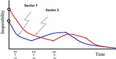
Level of inoperability trajectory in case of system deterioration
We can see that the level of inoperability of sector 1 displays an upward trend at time t = 2 weeks due a new perturbation then decays again following the DIIM trajectory. The same applies to sector 2 at time t = 3 weeks, where its recovery trajectory undergoes an increase then decays again following the inherent sector resilience trend.
Case 2: A new perturbation occurs and decreases the level of inoperability
This case corresponds to the introduction of mitigation strategies such as vaccines or antivirals. Such plans could alleviate the effect of influenza and reduce the level of inoperability. Figure 2 illustrates a new perturbation leading to a decrease in the level of inoperability.
Fig. 2.
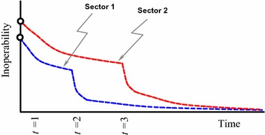
Level of inoperability trajectory in case of system improvement
At time t = 2 weeks, the level of inoperability trajectory of sector 1 drops abruptly and then reverts to the inherent path of recovery. On the other hand, the level of inoperability trajectory of sector 2 decreases suddenly at time t = 3 weeks and then goes back to the inherent path. The probability level p(t) is the factor that determines the weight given to the level of inoperability generated by the new perturbation and the level of inoperability generated by the DIIM model. In this work, the simulation is based on multiple phases of increasing complexity depending on the value of the probability of the new perturbation.
Simulation procedure
In this research work, we model the inoperability level of economic sectors by combining inoperability level resulting from both DIIM and the new perturbation. The overall inoperability level is calculated as an expected value of the inoperability level from DIIM and inoperability from the new perturbation. This is expressed mathematically in Eq. (1).
Figure 3 illustrates how the DIIM inoperability and new perturbation inoperability are combined into the computation of the overall inoperability of economic sectors.
Fig. 3.
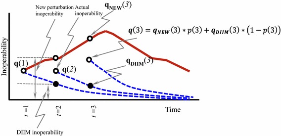
Inoperability level computation
The inoperability from the DIIM is calculated using the dynamic model expressed as follows (Haimes et al. 2005):
| 2 |
where q(t) is the level of inoperability vector at time t, K is the resilience matrix, and is the demand perturbation at time t.
The DIIM model computes the inoperability level at time t + 1 based on the inoperability level at time t plus the inoperability resulting from the resilience of the economic sector and the interdependencies with other economic sectors. The term is usually zero or negative, reducing the level of inoperability q(t) as measured at time t. The impact of the sector resilience is captured by the diagonal matrix K, whose elements measure the tendency of economic sectors to recover to their pre-disaster state after a given perturbation. To capture the effect of indirect inoperability and resilience effect, the matrix K is multiplied by the indirect impact caused by other sectors, , plus the reduced final demand, , minus the inoperability level at time t, q(t). Multiplying the economic sector resilience coefficient in the matrix K by generates a joint measure of resilience based on the level of interdependencies with other economic sectors as captured by the matrix, . Such approach enables the measurement of the inoperability level of a sector given its inherent resilience and also taking into consideration its dependence on other economic sectors. For instance, an economic sector might be very resilient to the disaster, but its high dependence on other inoperable sectors will cause its productivity to suffer at a much higher rate. As such, the DIIM model provides a measure of the time-varying inoperability levels of economic sectors resulting from both the direct impact from the disaster and the indirect impact from its dependence on other sectors.
The entries in the resilience matrix K are computed as follows:
| 3 |
where s i is a sector characteristic that depends on the initial inoperability level, T i is the recovery period for sector i, and a *ii are the diagonal elements of the interdependency matrix . Note that the inherent resilience coefficient k i is inversely proportional to recovery period T i and to the sector’s dependence on other sectors (1 − a *ii). This means that the shorter the recovery period and the lesser the dependence on other sectors, the higher the resilience coefficient k i. The detailed formulation of the DIIM sector resilience coefficient is provided by Lian and Haimes (2006).
Aside from the DIIM, another source of inoperability can be calculated based on the trend of the new perturbation, whether it is leading to the deterioration or improvement of economic sectors. In the case where the new perturbation leads to the deterioration of the economic system, the inoperability level follows an increasing trend that could be modeled using a wave function based on consolidated data from FluWorkLoss. A Matlab-based simulation formulates the wave function through a time-dependent base function f base(t) defined over the time horizon [a,b] that describes the time range of the new perturbation, where t represents week time increments. At time t = a weeks, a new perturbation occurs leading to the deterioration of the economic sectors. Due to the new perturbation, the inoperability level increases and the inoperability trajectory follows an upward trend, which is modeled using a base function based on consolidated data from FluWorkLoss. The base function is defined by two wave functions, which are assumed to be triangularly distributed. The first wave spans over the weekly time interval [0,28] and is defined as a triangular distribution between 0 and 28 weeks, with a peak inoperability level of 0.045 at week 20. Similarly, the second wave spans over the time interval [28,42] and is described as a triangular distribution between 28 and 42 weeks, with a peak inoperability level of 0.09 at week 35.
Therefore, the inoperability at time t = a week is computed as follows:
| 4 |
where
| 5 |
| 6 |
The quantity represents the inoperability level as computed by the DIIM modeling, and represents the inoperability level resulting from the new perturbation. The value of is calculated by multiplying the value from the base function f base(a) and the workers’ contribution vector w, which gives a vector of inoperability level for the 65 sectors due to the occurrence of the new perturbation. Both quantities and are combined into a weighted average using the probability of a new perturbation occurring p(a), which is drawn from a beta distribution with a specified mode value. We draw a finite number of probability values p(a) from the beta distribution to perform our Monte Carlo simulation. Therefore, we obtained a set of inoperability values for the 65 economic sectors at time t = a weeks. The computed inoperability values are stored in a three-dimensional matrix with dimensions representing economic sectors, time, and simulation iterations.
For time t = a + 1 week and subsequent times, the inoperability level is computed in the same manner until time t = b week when the effect of the new perturbation is over. At time t = b + 1 week, the effect of the new perturbation dissipates, and the subsequent inoperability path follows a decaying trend as sectors regain progressively their pre-disaster state. Then, from time t = b + 1 week and subsequent time increments, inoperability level is calculated using DIIM as follows:
| 7 |
In the case where the new perturbation leads to the improvement of the economic sectors, the inoperability level follows a decreasing trend that could be modeled by linking the inoperability at time t to the inoperability level at time t − 1. This could be constructed mathematically as follows:
| 8 |
where k is a scaling factor between 0 and 1 that depends on the intensity and the spread of the new perturbation leading to inoperability level decrease. The coefficient k is determined based on expert judgment given the nature of the influenza pandemic, the type of risk mitigation strategies used, and their deployment. For example, for medium intensity influenza pandemic with a probability of occurrence of 0.25, the large deployment of a portfolio of strategies comprising of vaccines, social distancing, and antivirals would correspond to a coefficient value of 0.2.
Therefore, at time t = a week, the inoperability level is computed by integrating the new perturbation inoperability and the DIIM inoperability as follows:
| 9 |
where
| 10 |
| 11 |
After time t = b week, the inoperability level is calculated based on only DIIM, showing a decaying trend until sectors regain their initial state. Based on the Monte Carlo simulation, we obtained a large data set that could be used to build distributions of inoperability for each economic sector throughout the recovery horizon. Moreover, we could compute the cumulative economic loss and their probability distributions at every increment of time. This is illustrated in Fig. 4.
Fig. 4.
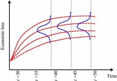
Economic loss modeling distribution
Beta distribution modeling
In this research work, we model the probability of the occurrence of a new perturbation through a beta distribution over the range [0,1]. We develop a simulation algorithm for beta distributions with a given mode value that serves as a calibration of the contribution of the impacts of both DIIM and the new disruption on economic sectors. The simulation in this research is based on Monte Carlo simulation through random number generation from a given probability distribution (Gentle 1998). Therefore, the probability p(t) could be considered as a random variable that follows a beta distribution. The beta distribution is used to model probabilities and proportions. It is defined between 0 and 1, and the shape of the distribution is determined by two parameters. The beta distribution has the property of modeling a set of symmetric or skewed points. The beta distribution is a candidate distribution to use since it has the capability to model bounded random variables such as probability values with support of [0,1]. Many studies have used the beta distribution in modeling proportions and subjective beliefs of individuals (Alvarez and Brehm 1995, 1997; Brehm and Scott 1993; Mebane 2000; Paolino 1998). The beta distribution is particularly suitable for modeling the level of perturbation (as well as the resulting inoperability), which is known to have a lower limit of 0 and an upper limit of 1. The bounded interval of the beta distribution provides an alternative to describe the uncertainty in probability of occurrence of a new perturbation. The beta distribution could be described by shape parameters α and β, which could be set to generate a distribution with a desired mode (or most likely value).
Economic loss modeling
Economic loss measure gives the monetary value of the degraded output of sectors. It is a different but complementary metric to assess the consequences of a disaster, such as a disease pandemic. In contrast to the level of inoperability, it is a more intuitive way to convey how critically a sector has been impacted by the pandemic. Measuring economic loss allows generating a different ranking for critically impacted sectors. Also, the results will help identify the sector that incurs the highest monetary losses following the pandemic. More importantly, we can evaluate that the sector losses exceed a criticality threshold that may lead to an irrecoverable collapse of the economic sector. Economic loss equals multiplying the level of inoperability and the planned output level. Multiplying the percentage of output degradation by the normal output of the sector in dollar amount gives the monetary value of the loss incurred by the sector. Our analysis considers 1-week increments; hence, economic loss is mathematically expressed as follows:
| 12 |
where loss i(t) represents the cumulative monetary loss at time t, X i represents the output of sector i during a given year, and q i(t) denotes time t level of inoperability for sector i. Note that the number 52 denotes the number of weeks per year since the sector production is measured on a yearly basis.
Research simulation focus
In this work, we build the simulation based on previously published work by El Haimar and Santos (2013), which considered a baseline scenario to assess and prioritize the risk of a pandemic disaster through two risk metrics. In the present study, we considered the critical sectors in light of both risk metrics, namely inoperability level and economic loss. Figure 5 illustrates the operational framework used in the present research study.
Fig. 5.
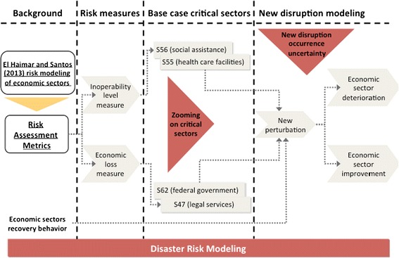
Disaster risk modeling framework
In particular, we examine the effect of a new perturbation on the most critical sector in terms of inoperability level, S56 (social assistance), as well as the sector with the highest economic loss value, S62 (federal government enterprises). We explore how the new perturbation could lead to the deterioration or improvement of inoperability level of sector S56, while taking into consideration the uncertainty in the probability of the occurrence of the new perturbation. In both cases, we capture the distribution of inoperability level at a given time for sector S56. On the other hand, we study how the new perturbation could lead to the deterioration in economic loss of critical sector S62, while modeling the probability of the new disruption using a beta distribution. Then, we look at how the new perturbation could lead to the improvement of the state of sector S62 by reducing economic loss.
Results and analysis
New perturbation leading to system deterioration
The first case developed in this research study is the examination of a new perturbation leading to economic sectors deterioration (i.e., a new surge of the pandemic or the evolution of the influenza virus).
Inoperability level
Figure 6 illustrates the inoperability simulation for sector S56. The top left graph illustrates the deterministic trajectory of the inoperability level for sector S56. We introduce the modeling of the new disruption by assuming a probability of occurrence that could be modeled using a beta distribution.
Fig. 6.
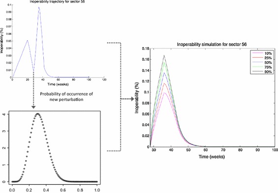
Inoperability simulation for sector S56
The graph on the right panel of Fig. 6 illustrates the different inoperability level percentiles trajectories. At time t = 28 weeks when the new perturbation occurs, there is a jump in the inoperability level. The inoperability level is calculated as an expected value of the inoperability level derived from the DIIM and the inoperability level resulting from the new disruption. The modeling of the probability of the new perturbation occurrence through a beta distribution gives a set of inoperability trajectories depending on the different values assigned to that probability. At time t = 42 weeks, when the new disruption starts to vanish, the inoperability level follows the DIIM’s decaying trend. The DIIM modeling incorporates economic sector resilience, which is assumed to reduce the effect of the disaster until it reverts to the pre-disaster state.
We look at the probability density function and the cumulative density function of inoperability level of sector S56 at time t = 35 weeks. Numerically, the inoperability level at time t = 35 weeks ranges from 3.84 to 19.98 % with a mean value of 13.45 %. Figure 7 displays the distribution of inoperability level for sector S56 at time t = 35 weeks. The graph at the top section of Fig. 7 displays the probability density of the inoperability level. We can see that the inoperability level follows a bell-shaped curve with an approximate average value of 13.45 % and a standard deviation of 2.65 %. Furthermore, the graph at the bottom right panel of Fig. 7 illustrates the cumulative density function of the inoperability level. The 90th percentile shows 17 % inoperability level, meaning that there is approximately 10 % probability that the inoperability level will be more than 17 %.
Fig. 7.
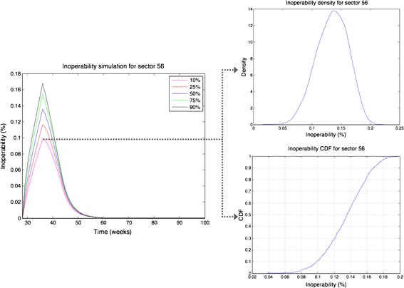
Inoperability distribution for sector S56
Economic loss
Figure 8 illustrates the trajectory simulation of economic loss for sector S62 throughout the recovery horizon. We can see that the economic loss of sector S62 sharply increases starting from time t = 28 weeks due to the occurrence of the new perturbation leading to the deterioration of the state of sectors.
Fig. 8.
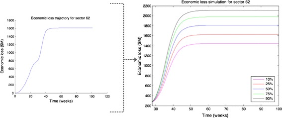
Economic loss simulation for sector S62
The plot shows various percentile trajectories of economic loss based on the modeling of the probability of occurrence of a new perturbation using a beta distribution. This trend creates an economic loss density function at each given point of time. To have a deeper understanding of the spread of economic loss scores, we investigated the distribution of economic loss of sector S62 at the end of the recovery period. Numerically, the simulation results generate economic loss values ranging from 922.42 ($M) to 2,359.6 ($M) with a mean value of 1,790.2 ($M). Figure 9 shows the distribution of economic loss for sector S62. The graph at the top right panel of Fig. 9 illustrates that the distribution of the economic loss has a bell-shaped curve that is nearly symmetric and centered around the mean value of 1,790.2 ($M) with a standard deviation value of 258.02 ($M). The graph at the bottom right panel of Fig. 9 illustrates the economic loss cumulative density for sector S62. Based on the results, there is a 90 % chance that the economic loss is going to exceed 2,100 ($M), while the median value is 1,812.1 ($M).
Fig. 9.
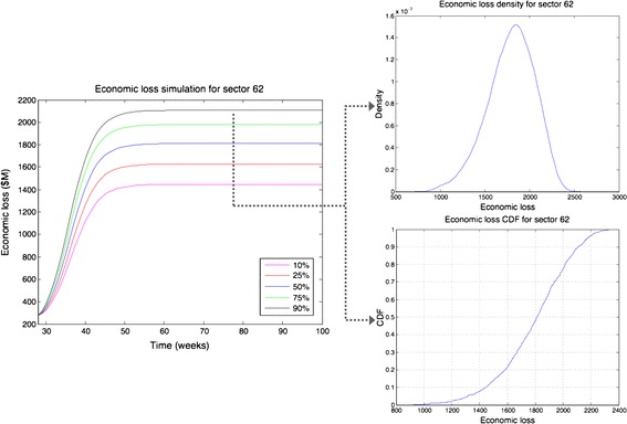
Economic loss distribution for sector S62
New perturbation leading to system improvement
The second case developed in this research study is the examination of a new perturbation leading to sector improvements in the case of mitigation strategies (e.g., vaccines, antivirals, social distancing). We examine the effect of system improvement on the critical sector in terms of inoperability (S56) and in terms of economic loss (S62).
Inoperability level
Figure 10 illustrates the inoperability simulation for sector S56 in the case of system improvement. We can see that the inoperability decreases starting from time t = 5 weeks, when the new disruption occurs. The new perturbation leads to reducing the inoperability level of economic sectors. This scenario is depicted as a sharp decrease in inoperability level values until the sectors regain their pre-disaster state.
Fig. 10.
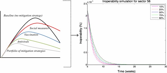
Inoperability simulation for sector S56
To closely examine the simulated inoperability level at the time of the new perturbation for sector S56, we inspected the probability density function of the inoperability level and the cumulative density function at time t = 8 weeks. Numerically, the inoperability level at time t = 8 weeks ranges from 7.70 × 10⁻⁷ % to 7.45 × 10⁻⁶ % with a mean value of 3.77 × 10⁻⁶ %. Figure 11 shows the distribution of the inoperability level of sector S56 at time t = 8 weeks. The top right graph shows that inoperability values are almost symmetrically spread around the average value of 3.77 × 10⁻⁶ %, with a calculated standard deviation of 1.25 × 10⁻⁶ %. The bottom right graph in Fig. 11 illustrates the cumulative density function of inoperability level for sector S56 at time t = 8 weeks with a median value of almost 3.75 × 10⁻⁶ %.
Fig. 11.
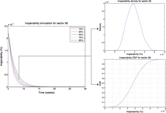
Inoperability distribution for sector S56
Economic loss
Figure 12 illustrates the economic loss trajectory simulation for sector S62 throughout the recovery period. We can see that the economic loss increases from t = 5 weeks, the time of occurrence of the new perturbation. Then, the cumulative economic loss stabilizes quickly due to the improvement generated in the economic system by the new perturbation. We also look at the economic loss density function and cumulative density for sector S62 at the end of the recovery. Numerically, the cumulative economic loss of sector S62 ranges from 0.7257 ($M) to 0.8795 ($M) with a mean value of 0.7837 ($M). Figure 13 shows the inoperability level distribution of sector S62 at the end of the recovery period. The economic loss has an approximately symmetric shape centered at the average value of 0.7837 ($M) with a standard deviation of 0.0245 ($M) and a median value of 0.7822 ($M).
Fig. 12.
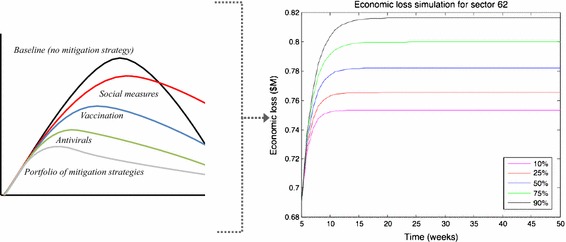
Economic loss simulation for sector S62
Fig. 13.
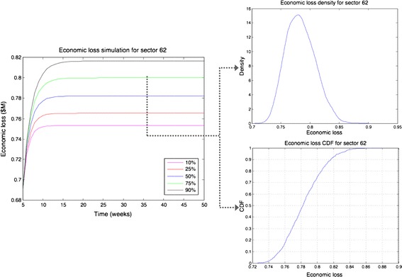
Economic loss distribution for sector S62
Analysis of results
The results developed in this study illustrate the inoperability level of sectors as a spectrum of trajectories that could be used to draw the probability distributions of inoperability level. Moreover, the uncertainty modeling of the probability of occurrence of a new perturbation also generates a spectrum of economic loss values that can be fitted into probability distributions. These new findings are attributable to various modeling complexities as explained below.
Integration of DIIM and new disruption modeling in creating inoperability level trajectories
The DIIM modeling takes into consideration the sector resilience factor in computing the inoperability of sectors. Economic resilience reflects the ability of a sector to regain momentum following a pandemic disaster and therefore determines the rate with which sectors go back to their pre-disaster state. Thus, the inoperability level due to the DIIM computation follows a decaying trend in the aftermath of the pandemic disaster. On the other hand, the new disruption modeling tries to capture the effect of any sudden perturbation to the path of the inoperability. Such perturbation could lead to either the improvement or the deterioration of the economic sectors. The combination of sector resilience modeling with new perturbations generates a more robust approach in developing the inoperability paths for the sectors. Moreover, the economic loss modeling is also subject to the effect of integrating both the DIIM and a new disruption. The new perturbation either amplifies the economic loss in the case of previously unforeseen system deterioration, or reduces the economic losses when risk management strategies are implemented.
Uncertainty modeling of the probability of occurrence of a new perturbation
In the present work, inoperability level is computed as an expected value of the inoperability from the DIIM and the inoperability from the new disruption. The weighting factor is the probability of occurrence of a new disruption, which is modeled as a beta distribution. The simulation algorithm generates samples from the probability distribution that give a set of inoperability trajectories. Modeling the probability of occurrence as a beta distribution is also reflected in the simulation of various economic loss trajectories.
According to the results developed in this research work, there are various phases in simulating the trajectory of inoperability.
Inoperability follows a path created using a combination of both DIIM and new disruption
When a new perturbation occurs, the inoperability levels of the economic sectors will become a function of both the DIIM and the new disruption. The DIIM incorporates the effect of resilience and sector interdependencies. Notably, the resilience parameter in the DIIM has the tendency to create a downward trend for the inoperability of a sector. On the other hand, the new perturbation has a certain trend that also influences the trajectory of inoperability of economic sectors. This new perturbation could have two possible trends:
Upward trend of inoperability in modeling the new perturbation leading to the deterioration of the system. Such disruption could be due to a new wave of influenza pandemic or the evolution of the virus. For instance, in the H1N1 pandemic of 2009, there were two consecutive waves of influenza that increased the inoperability level of economic sectors as modeled by FluWorkLoss. Specifically, as the first wave vanished, the sectors gained productivity momentum as workforce availability improved. However, another wave of influenza hit the workforce, and absenteeism rate further increased, which drives up the inoperability. An increase in inoperability level values leads to the deterioration of the economic system. Moreover, the degree of increase in the inoperability level depends on the level of criticality of the new disruption. For example, if the influenza virus mutates into a stronger type that spreads very quickly through humans, workforce availability will deteriorate leading to a significant increase in inoperability levels.
Downward pattern in inoperability when modeling the new disruption leading to the improvement of the system. Such perturbation could be due to the deployment of risk mitigation strategies such as vaccines, antivirals, or social distancing. Each risk mitigation strategy has its own effectiveness in reducing the impact of the disaster. The level of effectiveness of the risk mitigation strategy depends on the portfolio of measures taken and the intensity of their application. For instance, a portfolio of strategies could include a large deployment of both vaccines and social distancing measures in a community of sick individuals. Such measures can substantially curtail the impact of the influenza, therefore limiting the spread of the influenza virus. This implies that the absenteeism rate will tend to decrease, leading to higher productivity of economic sectors. This is reflected in a significant decay in the trajectory of inoperability.
Inoperability follows a decaying trend after the end of the new perturbation
The inoperability trajectory reverts to the DIIM trend when the effect of the perturbation ceases. Therefore, the inoperability level follows a decaying trajectory due to the resilience of economic sectors. Again, the rate of decay of inoperability level depends on the workforce dependence level and interdependencies across the sectors. However, the starting point of the decaying trend is dependent on the last value of inoperability observed after the new disruption is introduced. In the case of the deterioration of the system, the inoperability level at the end of the disruption is higher compared with the inoperability level at the beginning of the disruption. This means that the inoperability level of economic sectors will take longer to vanish due to the effect of the new perturbation. Therefore, we can see an apparent decaying trend of inoperability trajectory after the end of the new perturbation until the economic sector regains its pre-disaster state. In the case of the improvement of the system, the inoperability level will have significantly lower values at the end of the disruption. Hence, for such scenario, the inoperability level vanishes more quickly due to the resilience factor, and economic sectors regain their pre-disaster state more rapidly.
On the other hand, the simulation results have also exposed various phases associated with the trajectory of cumulative economic loss.
Economic loss trajectory follows an upward trend due to new disruption
When the new perturbation happens, the evolution trend of the cumulative economic loss changes depending on the nature of the new perturbation. Specifically, we distinguish two evolution trends:
The rate of increase in cumulative economic loss is steeper in the case of system deterioration. When the new perturbation suddenly occurs, leading to an increase in inoperability level, the productivity state of economic sectors worsens. The increase in inoperability level translates into an intensifying effect that drives economic loss to higher levels. This explains the abrupt jump in the economic loss trajectory.
The rate of increase in cumulative economic loss is slower in the case of system improvement. When the new disruption occurs, leading to inoperability level decay, the productivity state of sectors improves. The decay in inoperability level translates into a mitigating effect that reduces economic losses. Therefore, the economic loss trajectory increases slowly because of the mitigating impact of the new disruption.
Economic loss stabilizes in a steady state
At the end of the new disruption, the inoperability level of economic sectors decays slowly until it vanishes. Therefore, the inoperability level is insignificant to generate additional economic loss. Thus, the economic loss trajectory maintains a constant value throughout the rest of the recovery period.
A primary contribution of this research is the incorporation of the beta distribution to simulate the probability of a new perturbation occurring, which generates a spectrum of inoperability level and economic loss trajectories. Moreover, we create the probability distribution of inoperability level for the critical sector in terms of inoperability level, namely S56 (social assistance). Therefore, we could highlight the effect of any new disruption on the course of development of inoperability for the highly inoperable sectors. We also create the distribution of cumulative economic loss at the end of the recovery period, for the sector with the highest economic loss value, namely S62 (federal government enterprises), to focus on the overall economic impact of the pandemic on sectors.
In addition to the modeling of exogenous new perturbations, there is also the possibility of endogenous disruptions that could constitute a potential secondary perturbation. An example of this would be the inoperability emanating from dysfunctionality of health-care service sectors. This explains the ranking of sectors S56 (social assistance) and S55 (health-care facilities) as the two most adversely impacted sectors in terms of inoperability level (El Haimar and Santos 2013). First, the personnel in these sectors come into a direct contact with the sick individuals; therefore, they have a much higher probability of contracting the influenza virus. Second, these sectors experience a state of being overwhelmed due to the higher number of cases they receive. Thus, it is important to highlight that a new disruption leading to the deterioration of the economic system could be also due to endogenously generated secondary perturbations.
Conclusions and areas for future research
This paper analyzes the impacts of influenza disasters through consideration of two risk metrics, namely level of inoperability and economic loss. Also, the prioritization plans and critical sector identification were based on one of the two dimensions, meaning that we rank either the criticality of sectors through their level of inoperability values or their economic loss scores. One potential addition to the present study would be the evaluation of the efficacy of risk mitigation strategies (vaccines, antivirals, social distancing, etc.) in light of the findings of this stochastic analysis. A rigorous study of the effectiveness of the different risk mitigation strategies given the uncertainty of occurrence of a new perturbation would give realistic insights on the recovery trajectory of economic sectors. Therefore, the evaluation of risk mitigation strategies should take into consideration the eventual outcome of the new disruption as well as the probability of its occurrence. For instance, in the case where several risk mitigation strategies are deployed, the inoperability level of economic sectors is expected to decrease. Hence, the appropriate combination of risk mitigation strategies as well as the intensity of the application becomes an important issue to address. Another important feature that should be scrutinized is the combination effect of a perturbation leading to system deterioration and a perturbation leading to system improvement. Specifically, a new disruption leading to system deterioration would tend to increase inoperability level of economic sectors, while a new disruption leading to system improvement would tend to decrease inoperability level of the economic sectors. The recovery trajectory of economic sectors would then be subject to two competing effects. Therefore, to have a holistic analysis of the recovery behavior of sectors, it is imperative to study the effects collectively and generate risk management policies accordingly.
A primary objective of this research is the development of a practical framework for establishing public health policies particularly in terms of prioritizing limited medical personnel or resources. The results of such modeling framework would provide insights into the behavior of critically affected sectors in the event of unprecedented perturbations within the recovery timeline. For instance, sector S56 (social assistance) was the most affected sector in terms of the inoperability level. Further deterioration in the state of critical sectors, such as S56, could further escalate the public health crisis. Hence, critical sectors should be identified and given priority in the event of major disaster such as a pandemic to enable effective deployment of essential personnel and allocation of scarce resources. Furthermore, a novel contribution of this research is the integration of DIIM as a tool for risk analysis, coupled with the modeling a potential stochastic perturbations that could lead to either the deterioration or improvement of economic sectors. Such stochastic analysis would help describe the state of economic sectors and how they react when they are exposed to different scenarios and outcomes. The case studies we demonstrated in this paper can be extended to perform supplementary sensitivity analyses (e.g., by varying recovery times, levels of inoperability, and probability assumptions), which will eventually result in the formulation of robust disaster risk management strategies for health policy making.
In the present research, we extended the base case scenario developed by El Haimar and Santos (2013) to account for a new perturbation occurring and to incorporate uncertainty analysis in the modeling of the recovery behavior of economic sectors. In the baseline scenario for the NCR sectors, federal services and legal services incurred the highest economic losses given their significant output in the region. These sectors have a high GDP due to their huge presence in the region and the large number of employees that work in those sectors. On the other hand, medical service sectors were the ones to report the highest level of inoperability. This is due to the fact that medical service workforce attends to a large population of sick individuals and causes strain to the sector’s already limited capacity. Also, due to their constant interaction with infected individuals, medical personnel tend to have a high susceptibility to contract the influenza virus and therefore incur a high rate of workforce absenteeism. Therefore, we highlighted the effect of any new disruption happening on the critically classified sectors in light of the inoperability level and economic loss metrics, which are S56 (social assistance) and S62 (federal government enterprises), respectively. We modeled the impact of a new perturbation leading to deterioration in terms of both risk metrics for the respective economic sectors. The inoperability level was computed as a weighted average of the inoperability level derived from the DIIM and the inoperability level triggered by the new perturbation.
The results obtained from the simulation exhibit various phases in terms of both risk metrics, namely inoperability level and economic loss. The first phase is determined by the combined effect of both DIIM and new perturbation. When the new perturbation leads to system deterioration, there is a significant increase in inoperability level and therefore a significant increase in economic loss. When the new disruption causes system improvement, there is a significant decline in inoperability level and therefore an insignificant change in economic loss. The second phase is a stabilization phase in which the inoperability level calculation is determined solely by DIIM. The inoperability level trajectory decays slowly until it vanishes, and the economic loss trajectory follows a steady state, indicating that the sector has recovered to the pre-disaster state. Using the beta distribution, the recovery behavior of economic sectors was modeled through a spectrum of trajectories that reflect percentiles.
Acknowledgments
This work was partially funded by National Science Foundation (Award #1361116) in addition to the Department of Engineering Management and Systems Engineering (EMSE) at George Washington University (GWU). The findings and analysis in this work do not reflect the official positions of NSF and GWU.
References
- Akhtar R, Santos JR. Risk-based input–output analysis of hurricane impacts on interdependent regional workforce systems. Nat Hazards. 2013;65(1):391–405. doi: 10.1007/s11069-012-0369-0. [DOI] [Google Scholar]
- Alvarez RM, Brehm J. American ambivalence towards abortion policy: development of a heteroskedastic probit model of competing values. Am J Polit Sci. 1995;39(4):1026–1055. doi: 10.2307/2111669. [DOI] [Google Scholar]
- Alvarez RM, Brehm J. Are Americans ambivalent toward racial policies? Am J Polit Sci. 1997;41(2):345–374. doi: 10.2307/2111768. [DOI] [Google Scholar]
- Bartlett JG. Planning for avian influenza. Ann Intern Med. 2006;154:141–144. doi: 10.7326/0003-4819-145-2-200607180-00133. [DOI] [PubMed] [Google Scholar]
- Brehm J, Scott G. Donut shops and speed traps: evaluating models of supervision on police behavior. Am J Polit Sci. 1993;37(2):555–581. doi: 10.2307/2111384. [DOI] [Google Scholar]
- Centers for Disease Control and Prevention (CDC) (2010) CDC Estimates of 2009 Influenza cases, hospitalizations and deaths, April–December 12, 2009. http://cdc.gov/h1n1flu/estimates˙2009˙h1n1.htm. Accessed 15 Jan 2010
- Centers for Disease Control and Prevention (CDC) (2012) Update: influenza activity—United States, 2009–2010 season, Morbidity and Mortality Weekly Report (MMWR), 59(29): 901–908. http://www.cdc.gov/mmwr/preview/mmwrhtml/mm5929a2.htm. Accessed 16 Feb 2012 [PubMed]
- Centers for Disease Control and Prevention (CDC) (2014) National Center for health statistics mortality surveillance data. http://www.cdc.gov/flu/weekly/nchs.htm. Accessed 24 Oct 2014
- Chao DL, Halloran ME, Obenchain CJ, Longini IM. FluTE, a publicly available stochastic influenza epidemic simulation model. PLoS Comput Biol. 2010;6(1):e1000656. doi: 10.1371/journal.pcbi.1000656. [DOI] [PMC free article] [PubMed] [Google Scholar]
- Considine J, Shaban RZ, Patrick J, Holzhauser K, Aitken P, Clark M, Fielding E, FitzGerald G. Pandemic (H1N1) 2009 influenza in Australia: absenteeism and redeployment of emergency medicine and nursing staff. Emerg Med Aust. 2011;23:615–623. doi: 10.1111/j.1742-6723.2011.01461.x. [DOI] [PubMed] [Google Scholar]
- Department of Homeland Security, National Infrastructure Protection Plan (NIPP) (2009) http://www.dhs.gov/files/programs/editorial_0827.shtm
- Department of Homeland Security, National Response Framework (NRF) (2008) http://www.fema.gov/NRF
- Dhankhar P, Zhang X, Meltzer MI, Bridges CB (2006) FluWork-Loss 1.0: a manual to assist state and local public health officials in estimating the impact of an influenza pandemic on work day loss. Centers for Disease Control and Prevention, U.S. Department of Health and Human Services, Atlanta
- El Haimar A, Santos JR. Modeling uncertainties in workforce disruptions from influenza pandemics using dynamic input–output analysis. Risk Anal. 2013 doi: 10.1111/risa.12113. [DOI] [PubMed] [Google Scholar]
- Ferguson NM, Cummings DAT, Fraser C, Cajka JC, Cooley PC. Strategies for mitigating an influenza pandemic. Nature. 2006;442:448–452. doi: 10.1038/nature04795. [DOI] [PMC free article] [PubMed] [Google Scholar]
- Fraser C, et al. Pandemic potential of a strain of influenza A (H1N1): early findings. Science. 2009;324(5934):1557–1561. doi: 10.1126/science.1176062. [DOI] [PMC free article] [PubMed] [Google Scholar]
- Gentle JE. Random number generation and Monte Carlo methods. New York: Springer; 1998. [Google Scholar]
- Germann TC, Kadau K, Longini IM, Macken CA. Mitigation strategies for pandemic influenza in the United States. PNAS. 2006;103(15):5935–5940. doi: 10.1073/pnas.0601266103. [DOI] [PMC free article] [PubMed] [Google Scholar]
- Haimes YY, Horowitz BM, Lambert JH, Santos JR, Lian C, Crowther KG. Level of inoperability input–output model for interdependent infrastructure sectors. I: theory and methodology. J Infrastruct Syst. 2005;11(2):67–79. doi: 10.1061/(ASCE)1076-0342(2005)11:2(67). [DOI] [Google Scholar]
- Halder N, Kelso JK, Milne GJ. Analysis of the effectiveness of interventions used during the 2009 A/H1N1 influenza pandemic. BMC Public Health. 2010;10(168):1–14. doi: 10.1186/1471-2458-10-168. [DOI] [PMC free article] [PubMed] [Google Scholar]
- Hawryluck L, Lapinsky SE, Stewart TE. Clinical review: SARS-lessons in disaster management. Crit Care. 2005;9:384–389. doi: 10.1186/cc3041. [DOI] [PMC free article] [PubMed] [Google Scholar]
- Isard W. Methods of regional analysis: an introduction to regional science. Cambridge: MIT Press; 1960. p. 1960. [Google Scholar]
- Jiang P, Haimes YY. Risk management for Leontief based interdependent systems. Risk Anal. 2004;24(5):1215–1229. doi: 10.1111/j.0272-4332.2004.00520.x. [DOI] [PubMed] [Google Scholar]
- Jung J, Santos JR, Haimes YY. International trade level of inoperability input–output model (IT-IIM): theory and application. Risk Anal. 2009;29(1):137–154. doi: 10.1111/j.1539-6924.2008.01126.x. [DOI] [PubMed] [Google Scholar]
- Kujawski E. Multi-period model for disruptive events in interdependent systems. Syst Eng. 2006;9(4):281–295. doi: 10.1002/sys.20057. [DOI] [Google Scholar]
- Leontief W. Quantitative input and output relations in the economic system of the United States. Rev Econ Stat. 1936;18(3):105–125. doi: 10.2307/1927837. [DOI] [Google Scholar]
- Lian C, Haimes YY. Managing the risk of terrorism to interdependent infrastructure systems through the dynamic level of inoperability input–output model. Syst Eng. 2006;9(3):241–258. doi: 10.1002/sys.20051. [DOI] [Google Scholar]
- Mebane WR. Coordination, moderation, and institutional balancing in american presidential and house elections. Am Polit Sci Rev. 2000;94(1):37–58. doi: 10.2307/2586379. [DOI] [Google Scholar]
- Miller RE, Blair PD. Input–output analysis: foundations and extensions. 2. Cambridge: University Press; 2009. [Google Scholar]
- Orsi MJ, Santos JR. Probabilistic modeling of workforce-based disruptions and input–output analysis of interdependent ripple effects. Econ Syst Res. 2010;22(1):3–18. doi: 10.1080/09535311003612419. [DOI] [Google Scholar]
- Paolino P (1998) Voters’ perceptions of candidate viability: uncertainty and the prospects for momentum. Prepared for presentation at the 1998 Annual Meeting of the Midwest Political Science Association
- President of the United States (2003) Homeland security presidential directive 7: critical infrastructure identification, prioritization, and protection. http://www.fas.org/irp/offdocs/nspd/hspd-7.html
- President of the United States (2011) Presidential policy directive 8: national preparedness. http://www.dhs.gov/xabout/laws/gc_1215444247124.shtm
- Resurreccion JZ, Santos JR (2011) Developing an inventory-based prioritization methodology for assessing level of inoperability and economic loss in interdependent sectors. In: IEEE proceedings of systems and information engineering design symposium, pp 176–181
- Ruiz-Juri N, Kockelman KM. Evaluation of the trans-texas corridor proposal: application and enhancements of the random-utility-based multiregional input–output model. J Transp Eng. 2006;132(7):531–539. doi: 10.1061/(ASCE)0733-947X(2006)132:7(531). [DOI] [Google Scholar]
- Santos JR, Orsi MJ, Bond EJ. Pandemic recovery analysis using the dynamic level of inoperability input–output model. Risk Anal. 2009;29(12):1743–1758. doi: 10.1111/j.1539-6924.2009.01328.x. [DOI] [PubMed] [Google Scholar]
- Santos JR, May L, El Haimar A. Risk-based input–output analysis of influenza epidemic consequences on interdependent workforce sectors. Risk Anal. 2012 doi: 10.1111/risa.12002. [DOI] [PMC free article] [PubMed] [Google Scholar]
- Schanzer DL, Zheng H, Gilmore J. Statistical estimates of absenteeism attributable to seasonal and pandemic influenza from the Canadian Labour force survey. BMC Infect Dis. 2011;11(90):1–9. doi: 10.1186/1471-2334-11-90. [DOI] [PMC free article] [PubMed] [Google Scholar]
- Statistics Canada (2013) Impact of H1N1 and seasonal flu on hours worked. http://www.statcan.gc.ca/daily-quotidien/100115/dq100115c-eng.htm. Accessed 5 Jan 2013
- The Infrastructure Security Partnership (TISP) (2006) Regional disaster resilience: a guide for developing an action plan, Document #19458. American Society of Civil Engineers, Reston
- US Department of Commerce . Regional multipliers: a user handbook for the regional input–output modeling system. Washington: U.S. Government Printing Office; 1997. [Google Scholar]
- World Health Organization (2003) Influenza. http://www.who.int/mediacentre/factsheets/2003/fs211/en/
- World Health Organization (2010) H1N1 in post-pandemic period. http://www.who.int/mediacentre/news/statements/2010/h1n1˙vpc˙20100810/en/index.html. Accessed 5 Oct 2010
- Xu W, et al. Supply-driven dynamic level of inoperability input–output price model for interdependent infrastructure systems. J Infrastruct Syst. 2011;17(4):151–162. doi: 10.1061/(ASCE)IS.1943-555X.0000058. [DOI] [Google Scholar]


