Abstract
When a bistable visual image, such as the Necker cube, is continuously viewed, the percept of the image endogenously alternates between one possible percept and the other. However, perceptual alternation can also be induced by an exogenous perturbation. For example, a typical external perturbation is the flashlight, which is expected to pervasively activate many brain regions. Therefore, the neural mechanism related to exogenous perceptual alternation remains to be clarified. As a cue to solving this problem, our recent psychophysiological experiment reported a positive correlation between the enhancement of visual mismatch negativity evoked by breaks in the sequential regularity of the visual stimuli and the proportion of perceptual alternation. To elucidate the mechanism underlying exogenous perceptual alternation induced by visual mismatch negativity, the present study attempted to construct a neural network model for bistable perception of the Necker cube, whose perceptual alternation is facilitated by an increase in visual mismatch negativity. The model consists of both a prediction layer and a prediction error layer, following the predictive coding framework for biologically plausible relationships between the change detection process and the perceptual alternation mechanism. Computer simulations showed that the mean duration of perception decreased as the response increased, which is in concordance with the experimental data. This result suggested that the excitatory feedforward and inhibitory feedback connections play an important role. Additionally, the validity of this model suggests that the visual mismatch signal propagates in the neural systems and affects the visual perceptual mechanism as a prediction error signal.
Keywords: Necker cube, Perceptual alternation, Neural network model, Predictive coding
Introduction
When a bistable visual stimulus, such as binocular rivalry and the Necker cube, is continuously viewed, the percept of the image endogenously alternates between one possible percept and the other (Leopold and Logothetis 1999; Sterzer et al. 2009). In particular, the perceptual alternation in binocular rivalry was examined vigorously (Brascamp et al. 2015). For example, the distribution of the duration of a percept showed a long-tail, like the gamma distribution (Levelt 1968), whereas the coefficient of variation (CV) of the duration was between 0.4 and 0.6 (Shpiro et al. 2009). Since the strength of the stimulus from each eye can be manipulated independently in binocular rivalry, many experimental results were reported under various conditions. For example, increase of the stimulus strength in one eye reduces the perceptual duration of the other eye and increases the perceptual alternation rate, which are known as Levelt’s Propositions 2 and 3 (Levelt 1968), respectively. However, recent findings suggested that such prepositions should be revised (Moreno-Bote et al. 2010; Brascamp et al. 2015; Wilson 2007; Levelt 1968; Platonov and Goossens 2013). These revised propositions appear to be more general than the original ones as they account for the recent findings and the previous data obtained in the early experiments.
Many computational models assuming dynamics or stochastic process were proposed to elucidate the mechanism underlying binocular rivalry (Curtu et al. 2008; Laing and Chow 2002; Lehky 1988; Matsuoka 1984; Moreno-Bote et al. 2007; Pisarchik et al. 2014; Runnova et al. 2016; Shpiro et al. 2007, 2009; Stollenwerk and Bode 2003; Panagiotaropoulos et al. 2013; Wilson 2007; Buesing et al. 2011; Gershman et al. 2012; Dayan 1998). The models reproducing the experimental data share the following common assumptions (Brascamp et al. 2015; Shpiro et al. 2007): (1) the perception corresponds to the high activity of a different neuronal population, (2) these populations inhibit each other, (3) the populations and/or the inhibitory connections gradually reduce efficacy, and (4) their activities are subject to random fluctuations. Notably, the models predicted the revised Levelt’s propositions (Wilson 2007; Moreno-Bote et al. 2010; Shpiro et al. 2007; Curtu et al. 2008; Platonov and Goossens 2013) before each phenomenon was experimentally reported. Consequently, a neural population model with slow adaptation and mutual inhibition may satisfy the fundamental characteristics of perceptual alternation.
In contrast, the stimulus is identical for both eyes in the Necker cube. Therefore, an experiment with different visual stimuli to the left and right eye is not possible. Computational models on perceptual alternations of the Necker cube have been also proposed as those for binocular rivalry (Sundareswars and Schrater 2008; Grossber and Swaminathan 2004). In contrast to endogenous alternation, the perceptual alternation induced by a perturbation outside the brain is referred to as “exogenous perceptual alternation”. Although such perturbations are external, such as a flashlight, they were reported to cause perceptual alternation (Kanai et al. 2005) and such strong stimuli pervasively activate many brain regions. Therefore, the mechanism of exogenous perceptual alternation remains to be clarified.
As a breakthrough in this problem, a psychophysiological experiment recently reported that the facilitation of perceptual alternation induced by the detection of visual change in a temporal sequence was correlated to the visual mismatch negativity amplitude (vMMN) (Urakawa et al. 2017a). Generally, the vMMN represents an electroencephalographic brain response which is evoked by a visual change. In this previous study (Urakawa et al. 2017a), electroencephalography (EEG) was measured during a psychological task under a modified oddball paradigm. The paradigm involved the intermittent presentation of eight horizontal or vertical bars with the centered Necker cube and participants were asked to report the percept of the Necker cube (Fig. 1). In the deviant condition (DEV), the sequential regularity was broken by a change in bars orientation. In contrast, such orientations were kept constant in the control condition (STD). As a result, the perceptual alternation rate in the DEV was significantly larger than that observed in the STD. In addition, a positive correlation between the increase in perceptual alternation and the vMMN amplitude (that reflects visual change detection) was found. This implies that specific brain areas, which are relevant to the automatic visual change detection process reflected in vMMN, induce exogenous perceptual alternation (Urakawa et al. 2017b). Furthermore, this study suggests that the prediction error contributes to inducing the exploratory visual process in order to shape the upcoming percept of the bistable image. This kind of task-irrelevant stimuli was not considered in most of the previous models of perceptual alternation, and clarifying the mechanism by which visual change detection correlates with perception is yet to be defined.
Fig. 1.
Exogenous perceptual alternation induced by breaks in sequential regularity (Urakawa et al. 2017a)
This finding appears to be closely related to predictive coding theory (Friston 2003, 2005), where both internal prediction and sensory stimuli are considered. In fact, the predictive coding theory has been applied to similar neurophysiological and psychophysical phenomena, including endogenous perceptual alternation in binocular rivalry (Hohwy et al. 2008), mismatch negativity (MMN) (Stefanics et al. 2014; Wacongne et al. 2012; Lieder et al. 2013b), and categorization of visual stimuli (Spratling 2016). In this framework, the vMMN’s amplitude was suggested to correspond to the strength of prediction error in the temporal sequence (Urakawa et al. 2017a). Therefore, the reported enhancement of perceptual alternations evoked by the change detection may be uniformly interpreted by enhancement of the prediction error. On the other hand, previous models for perceptual alternations do not consider prediction errors by non-bistable visual images. The purpose of this study was to construct a neural network model for exogenous perceptual alternation for the Necker cube, which explains the perceptual alternation promoted by the vMMN’s enhancement. Considering visual change detection as one of visual processes relevant to yield the prediction error, we expect that a computational model which minimizes the prediction error, i.e., vMMN amplitude, will promote perceptual alternation, as the previous experiment has reported. There are many implementation strategies in predictive coding, from Bayes inferences to neural network models (Friston 2003, 2005; Hohwy et al. 2008; Clark 2013; Chikkerur et al. 2010; Lieder et al. 2013a; Stefanics et al. 2014; Wacongne et al. 2012). Besides the induction of perceptual alternation through the vMMN, our model should retain the dynamical characteristics of the established models to reproduce previous experimental data. In the current study, we extended the representative neural network model of perceptual alternations following predictive coding theory and succeeded in the simulation of previous experimental data. In addition, we showed that the simple addition of prediction error to the previous model cannot reproduce the experimental data, and we discussed the importance of the network structure. Our theoretical study supported the hypothetical mechanism suggested by our previous experiments.
Model and methods
Neural network model
Following the framework of the predictive coding theory, we constructed a neural network model comprised of two layers, namely the Prediction Layer (P-Layer) and the Prediction Error Layer (PE-Layer), as shown in Fig. 2. Furthermore, the P-Layer includes two neurons (, ), and each neuron assumes to insist each percept for the Necker cube with the strength of each firing rate. As in the predictive coding theory, each neuron sends a prediction signal to the PE-layer. To avoid simultaneous dual perceptions, relatively strong mutual inhibitive projections are assumed between the neurons in the P-Layer. In contrast, the PE-Layer consists of seven neurons, three excitatory neurons (–) and four inhibitory ones (–). Each excitatory neuron (–) receives a response for a part of the Necker cube, as shown in the circles displayed in Fig. 2, and sends in turn signals to one or both neurons in the P-Layer. In addition, they also receive negative feedback from the P-Layer neurons, by way of the rest inhibitory neurons (–). The connections between the PE-Layer and the P-Layer would be simply parallel if the stimuli from the left and right eye remained independent in the binocular rivalry (Hohwy et al. 2008). In the Necker cube, however, a stimulus is common to both eyes and the outer frame of the Necker cube commonly supports both perceptions. Therefore, two neurons (, ) were minimally set in the PE-Layer, the first supporting a perception and the second () supporting both perceptions (Fig. 2).
Fig. 2.
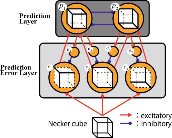
Proposed Neural Network Model. The model consists of two layers, namely the Prediction Layer and the Prediction Error Layer. The layers include 2 and 7 neurons, respectively. The red arrows indicate excitatory projections, while the blue arrows describe the inhibitory ones
The P-Layer neuron sends a negative feedback to the neuron that supports itself with an excitatory projection, which represents one of the features of the predictive coding theory. The excitatory input to an excitatory neuron in the PE-Layer symbolizes the response to bottom-up visual stimuli, while the inhibitory one is the feedback from the P-Layer. Therefore, the excitatory neuron in the PE-Layer is strongly activated when the visual stimulus is not correctly predicted. In contrast, when the prediction is correct, the firing rate of the PE-Layer neuron will be suppressed. In other words, the excitatory feedforward signal from the PE-Layer to the P-Layer corresponds to a prediction error. Therefore, the firing rate of a P-Layer neuron increases immediately after the presentation of a visual stimulus, but it gradually decreases as negative feedback suppresses the PE-Layer. From another viewpoint, the neural adaptation effect is implemented in the relationship between the P-Layer and the PE-Layer.
To produce the slow adaptation effect, inhibitory neurons are explicitly mediated between P-Layer and PE-Layer neurons. Without considering the perceptual biases, symmetric synaptic weights were assumed between neurons for simplicity (Table 1). Furthermore, to prevent multi-perceptions or non-perception, the weights were adjusted ensuring that the firing rate would be between and .
Table 1.
Synaptic weights of the network model
| Role | Connections | Weights |
|---|---|---|
| Stimulus response | , | 0.75 |
| 1.0 | ||
| Bottom-up | , | 2.0 |
| , | 1.6 | |
| Mutual inhibition | , | − 1.5 |
| Top-down | , | 0.6 |
| , | − 0.6 | |
| , | 0.48 | |
| , | − 0.48 |
As a duration of a percet in the computer simulations, we only count when the dominant neuron’s firing rate is 2 times higher than the other neuron to exclude momentary alternations under the noisy conditions. Another way of alternative perception does not affect the essential results. To prevent the effect of initial fluctuations in the simulation, the first 10 perceptual alternations were excluded from the analysis. Additionally, the cases in which perceptual duration was less than 100 time-steps were also not included.
Model neuron
We assume a simple integrate-and-fire model. The firing rate v of excitatory and inhibitory neurons in PE-Layer and a P-Layer neuron are defined respectively as follows:
| 1 |
| 2 |
| 3 |
where is the excitatory synaptic weight, represents the firing rate of an excitatory neuron, indicates the inhibitory synaptic weight, suggests the firing rate of an inhibitory neuron, W is the weight for an input, represents the time constant, f indicates the sigmoidal function: , and I is assumed to be the response in the lower visual cortex which is input to the excitatory neurons – in the PE-Layer. The time constants are and in excitatory (, , –) and inhibitory (–) neurons, respectively.
We assume two kinds of external inputs I to the model, (1) Gaussian noise + constant and (2) pulsed error signal (PE) + constant. These inputs are expected to induce endogenous and exogenous perceptual alternations, respectively, and are described in the next sections. The fourth-order Runge–Kutta method with a 0.01 incremental width was used in the numerical calculation of ordinary differential equations.
Gaussian inputs
First, we confirmed whether our model showed endogenous perceptual alternations, as observed in previous computational models. A constant , correspondent to a response to the Necker cube plus a fluctuation n imitating spontaneous activity, is input to every excitatory neuron - in the PE-Layer. In other words, I is an external input to this model, while n follows an Ornstein-Uhlenbeck process (Risken 1996), as shown below.
| 4 |
where is the time constant, represents the Gaussian noise with zero mean and unit variation, and indicates its strength. Figure 3 shows an example of external input. Since this fluctuation successively changes, it is often used in computer simulations of a neuron’s firing rate (Shpiro et al. 2009, for example).
Fig. 3.
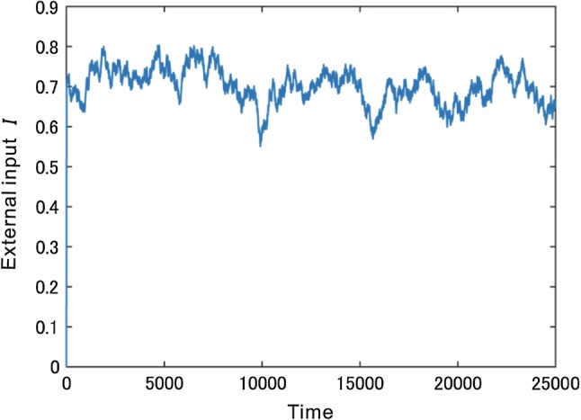
An example of Gaussian inputs (, )
Experimentally, the distribution of perceptual durations shows a right-skewed distribution, such as the Gaussian or logarithmic normal distribution (Levelt 1968; Zhou et al. 2004), where the CV is known to be approximately 0.5 (Levelt68). In the present study, we would like to confirm whether our model also shows the same characteristics for Gaussian noises (, ).
Pulsed inputs
To reproduce exogenous perceptual alternations, as achieved in previous experiments (Urakawa et al. 2017a), determining the way of introduction of the vMMN into our model is of great importance. Since the vMMN is thought to reflect a prediction error for unpredictable brakes in temporal irregularity (Stefanics et al. 2014), the external input to the PE-Layer neurons was assumed to reflect the vMMN. This hypothesis is supported by a previous investigation which also used the predictive coding model, as a deviant signal after regularity learning enables a prediction error neuron to fire similarly to an actual MMN (Wacongne et al. 2012). In this study, a constant response to the Necker cube and a response for the changes in the surrounding bars reflecting vMMN (prediction error), i.e. PE signal, was input to every excitatory neuron in the PE-Layer, where . In other words, we assume that the prediction errors for the bars produced elsewhere are broadly transmitted and reach the PE-Layer neurons for the Necker cube. For simplicity, PE-Layer neurons for the bars are not explicitly implemented in the model. The duration of bar stimuli and the interstimulus interval are 25 time-steps each. Moreover, 99% of the stimuli are standard while 1% are deviant. To clarify the effect of network dynamics on perceptual alternation, noise was not added in this simulation. Since the effect of noise, which is mainly limited to the fluctuations of perceptual duration, is much less than dynamics and diminished by averaging, major results would not be affected. The present study set five deviance magnitudes. The strength of the PE signal is 0.2 for the standard stimuli and 0.2, 0.3, 0.4, 0.6, 1.0 (5 conditions: , , , , ) for the deviant stimuli. An increase in the deviant to standard ratio suggests the occurrence of more augmented vMMN. The mean perceptual durations were compared assuming that the deviant stimulus was given once in a percept. Each deviance was added 475 times, where the timing was randomly chosen in each trial.
Results
Endogenous perceptual alternation
Before trying the Gaussian inputs, the constant external input was applied. Figure 4 shows the periodic perceptual alternation observed when the constant is uniformly input to every excitatory neuron in the PE-Layer. The percept duration was . Spontaneous perceptual alternation periodically occurred through two neuronal activity phases as follows: (1) Increased firing rate of the dominant P-Layer neuron and decreased rate of the other neuron, (2) decreased firing rate of the dominant P-Layer neuron and increased rate of the other neuron. In the 2nd phase, the increase (decrease) of the firing rate of a PE-Layer neuron underlies the increase (decrease) of the corresponding P-Layer neuron. This reverse tendency over these phases leads to perceptual alternation. In the predictive coding theory, perceptual alternation is considered a result of the accumulation in prediction error neurons of the prediction errors for unperceived stimulus (Hohwy et al. 2008).
Fig. 4.
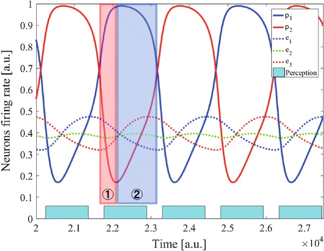
Firing rates in response to a constant. The solid line indicates the firing rate of a P-Layer neuron, whereas the dotted line represents the firing rate of an excitatory neuron in the PE-Layer. Each blue rectangle suggests the constant duration of a percept
When the Gaussian fluctuation is uniformly input to every excitatory neuron in the PE-Layer, Fig. 5 shows the firing rates of excitatory neurons in both the P-Layer and the PE-Layer. Briefly, the firing rates of and increased alternatively and periodically, and the occurrence of endogenous perceptual alternation was confirmed. Furthermore, perceptual duration showed a right-skewed distribution, where the mean was and the CV was 0.423 (Fig. 6). These are in concordance with the main properties of the experimental data previously reported (Shpiro et al. 2009; Brascamp et al. 2015). Since our perceptual alternation model reports structural mutual inhibition and slow adaptation, as previous models do, such a result is rather reasonable.
Fig. 5.
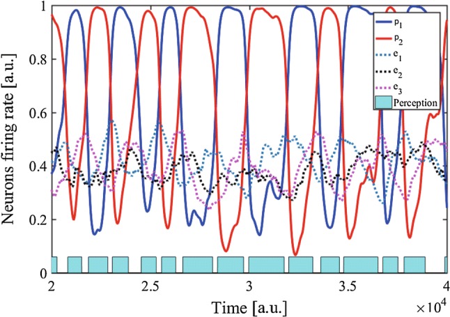
Firing rates in response to Gaussian fluctuations. The solid line indicates the firing rate of a P-Layer neuron whereas the dotted line represents the firing rate of an excitatory neuron in the PE-Layer. Each blue rectangle suggests the duration of a percept
Fig. 6.
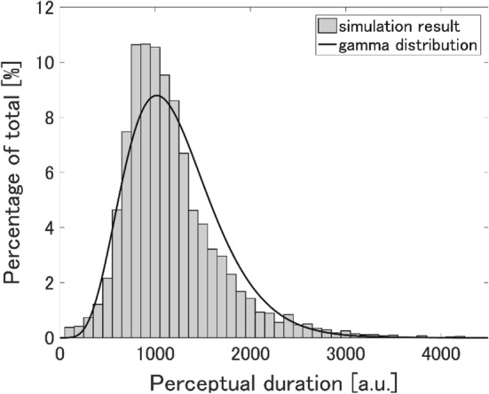
Distribution of perceptual durations
Exogenous perceptual alternation
To simulate exogenous perceptual alternation, a pulsed signal, resembling the responses to the Necker cube and the standard and deviant bars, was commonly input to every excitatory neuron in the PE-Layer. Reflecting the vMMN, the input pulse amplitude was larger in response to a 1% deviant stimulus of bars, although it was smaller for the 99% standard ones. Figure 7 shows the firing rates of excitatory neurons in both the P-Layer and the PE-Layer following the pulsed signals. We compared the durations of percept between the two conditions in various pulse amplitudes, in the presence of standard pulses only and when a deviant one was input among them. As a result, the duration of percept decreased as the response to deviance increased (Fig. 8). A repeated-measure one-way ANOVA was conducted in the statistical analysis using software SPSS (IBM). The main effect was significant (, ), and all pairs in the post-hoc test with Bonferroni corrections were significant (overall ). This result is correspondent with the experimental data in the previous study (Urakawa et al. 2017a, b).
Fig. 7.
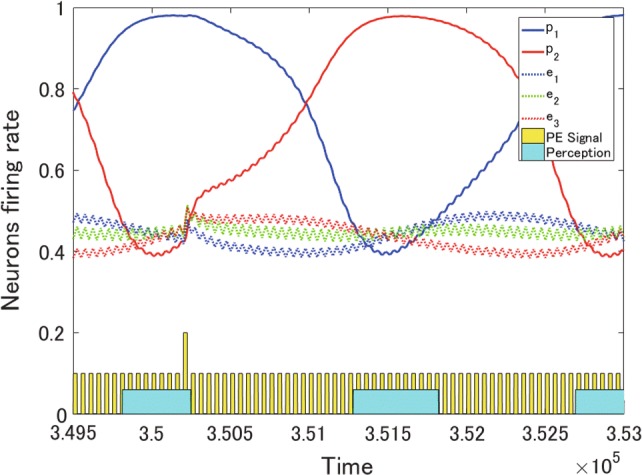
Firing rates in response to pulses. The solid line indicates the firing rate of a P-Layer neuron, whereas the dotted line represents the firing rate of an excitatory neuron in the PE-Layer. The yellow pulses describe PE signals. Each blue rectangle suggests the duration of a percept
Fig. 8.
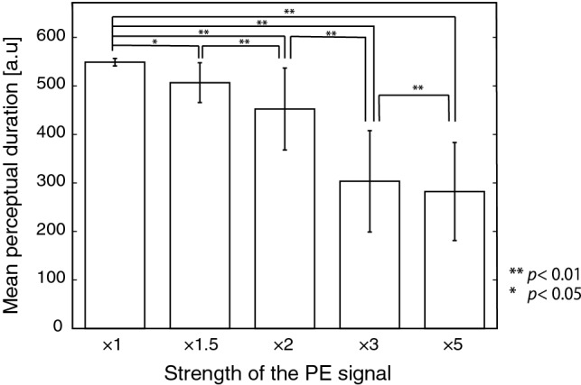
Relation between the mean perceptual duration and the amplitude of a deviant PE signal. Error bars show the standard deviation. Horizontal axis indicates the relative strength to the amplitude of a standard pulse
Discussion
By constructing a neural network model using both the prediction and the prediction error layers in the predictive coding framework, we succeeded in the simulation of previous experimental data related to exogenous perceptual alternation induced by the vMMN. In the proposed model, the vMMN effect was introduced into the volley of inputs, assuming that the prediction error evoked by a deviant stimulus would spread across visual processing areas. As a result of the computer simulations, the duration of a percept decreased, while the alternation was induced as the strength of the PE signal increased. This is in concordance with previous experimental results regarding the positive correlation between the perceptual alternation rate and the vMMN strength (Urakawa et al. 2017a, b). We also demonstrated that the model follows the experimental properties of endogenous perceptual alternation as well as the exogenous one, as reported in previous models. This is a result of presence of the typical dynamical characteristics of mutual inhibition and slow adaptation for perception in the present model, inherited from previous models (Shpiro et al. 2007; Brascamp et al. 2015). If the neural mechanism incorporated in our model is assumed, prediction errors induced through the change detection system are suggested to spread across visual perception areas.
Here, we show that a difference in the structure affects whether the experimental data shown in Fig. 8 can be reproduced or not. To show the difference clearly, we will compare the behaviors of two simple models. The first model is a representative model of conventional models (Laing and Chow 2002; Shpiro et al. 2007) as follows. The model consists of four model neurons as shown in Fig. 9a. and represent the activities of opponent neurons for percepts, while and indicate those of adaptation neurons. The input to the model, I, represents visual stimulus of the Necker cube. d is provided as a mismatch detection signal for deviant stimuli. They obey the following equations:
| 5 |
where and g are connection strengths between percept neurons and adaptation neurons, respectively. And f is a sigmoid function , where , and . For the second model, we simplified our model for comparability. The model consists of four model neurons as shown in Fig. 9b. and represent the activities of the percept neurons, while and indicate those of prediction error neurons. They obey the following equations:
| 6 |
where I is an input reflecting the bistable image, and d is a signal by the mismatch detection. and g are connection strengths between percept neurons and prediction error neurons, respectively. f is the same sigmoid function as shown above. The mismatch signal should be generated by the change detection of orientation of the bars, that is irrelevant to the task on the Necker cube. Thus, we assume that d is given from the outside to mediate Necker cube perception neurons, and as in Fig. 9b. In the previous model, d is given to and for the same condition (Fig. 9a).
Fig. 9.
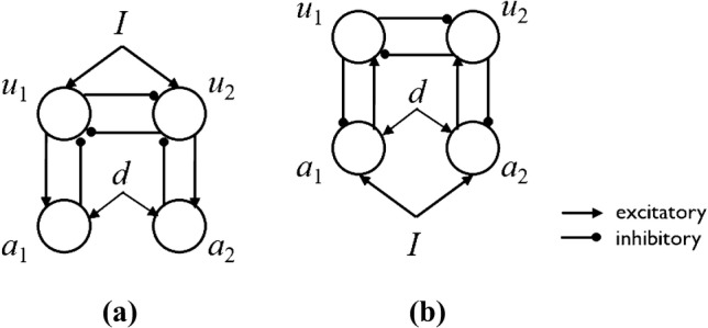
A conventional model (a) and the simplified proposed model based on predictive coding (b)
Figure 10 shows the simulation results of dominant durations for different d in the two models. The parameter values were as follows: β = 1.1, g = 0.5, and τ = 100. The inputs were and 3.0 for previous and proposed models, respectively. This difference is due to the range of I for bistable oscillations. The input strength is assumed to be relatively larger because it reflects the stimulus of a bistable image. The result means that the conventional model does not decrease as the fluctuation increases, although the proposed model does, as in Fig. 8. This indicates that the previous model (Fig. 9a) cannot reproduce the tendency shown in Fig. 8.
Fig. 10.
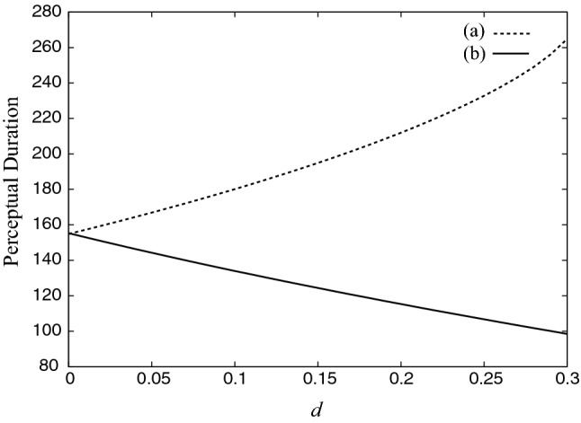
Change of perceptual duration for increase in fluctuation. The tendency is different for a the conventional model and b the proposed model, based on predictive coding
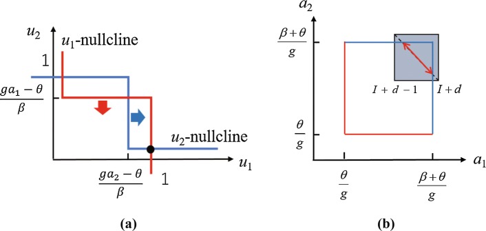
Furthermore, to intuitively understand these results, we attempted to provide theoretical explanations. Actually, we applied the analytical method of Curtu et al. (2008) to the simplified proposed model as follows. For simplicity, the sigmoid function was approximated by the Heaviside function h(x) with the threshold , where if , otherwise . According to the dynamical system Eq. (6), the nullclines are shown in Fig. 11a. Assuming that and , is decreasing (-nullcline is sliding down) and is increasing (-nullcline is sliding rightward). If either of the thresholds cross 0 or 1, the equilibrium point disappears and the system will be attracted to . This drastic change corresponds to perceptual alternation. At this moment, or . From symmetricity, when or , a perceptual alternation also occurs. The red and blue boundaries where perceptual alternation occurs are shown in Fig. 11b. On the other hand, and asymptotically change along the diagonal of the gray square in Fig. 11 because they slowly approach to and alternately. Therefore, the red arrow indicates the central pathway of . If d increases, the gray square moves toward the upper-right and the width of the arrow will decrease. This means that the period of the percept decreases as d increases as shown in Fig. 10. For the conventional model, similar analysis (Curtu et al. 2008) confirms the tendency in Fig. 10. It is clear that the tendencies are so robust that they are not affected by small changes in parameter values, but by the network structure. These show that for the network structure of previous models it is irrelevant to embed the mismatch signal to explain the experimental data. Therefore, the analyses indicate that the excitatory feedforward and inhibitory feedback connections, before perception, play an important role in reproducing the tendency. Besides, this structure fits well with the predictive coding framework.
Fig. 11.
Analysis of the dynamics of the proposed model (Curtu et al. 2008). a Nullclines on the plane (, ). b Dynamics on the plane (, ) show that the duration decreases as the value of d increases
In contrast, the mean perceptual duration did not decrease, in the case of the Gaussian inputs, implying perceptual alternation suppression. This property was attributed to the simple neural network dynamics with mutual inhibition and slow adaptation of the typical perceptual alternation models (Curtu et al. 2008; Shpiro et al. 2007). In summary, the perceptual duration increases as the stimulus input increases for smaller inputs, considering that the “release mechanism” (i.e., the input effect to a dominant population is relatively stronger) is dominant, while the duration decreases as the stimulus increases for larger inputs, as a result of the “escape mechanism” (the input effect to a suppressed population is relatively stronger). Since the amount of change in Gaussian signals per unit time is smaller than that of pulsed ones, the result of our numerical experiments is consistent with these explanations from the dynamical viewpoint. This confirms that our computational model shares the same dynamical property of the typical previous models. The model should reproduce Levelt’s prepositions as the previous models did. The essential difference lies in the implementation method for adaptation, which are represented by positive bottom-up and negative top-down neural projections in the predictive coding framework. In this structure, the vMMN signal can be introduced as a prediction error in a reasonable way. In the proposed model, inhibitory neurons with a larger time constant slow down the feedback, which consequently leads to slow adaptation.
Footnotes
Publisher's Note
Springer Nature remains neutral with regard to jurisdictional claims in published maps and institutional affiliations.
References
- Buesing L, Bill J, Nessler B, Maass W. Neural dynamics as sampling: a model for stochastic computation in recurrent networks of spiking neurons. PLoS Comput Biol. 2011;7(11):e1002211. doi: 10.1371/journal.pcbi.1002211. [DOI] [PMC free article] [PubMed] [Google Scholar]
- Brascamp JW, Klink PC, Levelt WJM. The laws of binocular rivalry: 50 years of Levelt’s propositions. Vis Res. 2015;109:20–37. doi: 10.1016/j.visres.2015.02.019. [DOI] [PubMed] [Google Scholar]
- Chikkerur S, Serre T, Tan C, Poggio T. What and where: a Bayesian inference theory of attention. Vis Res. 2010;50(22):2233–2247. doi: 10.1016/j.visres.2010.05.013. [DOI] [PubMed] [Google Scholar]
- Clark A. Whatever next? Predictive brains, situated agents, and the future of cognitive science. Behav Brain Sci. 2013;36(3):181–204. doi: 10.1017/S0140525X12000477. [DOI] [PubMed] [Google Scholar]
- Curtu R, Shpiro A, Rubin N, Rinzel J. Mechanisms for frequency control in neuronal competition models. SIAM J Appl Dyn Syst. 2008;7(2):609–649. doi: 10.1137/070705842. [DOI] [PMC free article] [PubMed] [Google Scholar]
- Dayan P. A hierarchical model of binocular rivalry. Neural Comput. 1998;10(5):1119–1135. doi: 10.1162/089976698300017377. [DOI] [PubMed] [Google Scholar]
- Friston K. Learning and inference in the brain. Neural Netw. 2003;16(9):1325–1352. doi: 10.1016/j.neunet.2003.06.005. [DOI] [PubMed] [Google Scholar]
- Friston K. A theory of cortical responses. Philos T Roy Soc B. 2005;360(1456):815–836. doi: 10.1098/rstb.2005.1622. [DOI] [PMC free article] [PubMed] [Google Scholar]
- Gershman SJ, Vul E, Tenenbaum JB. Multistability and perceptual inference. Neural Comput. 2012;24(1):1–24. doi: 10.1162/NECO_a_00226. [DOI] [PubMed] [Google Scholar]
- Grossber S, Swaminathan G. A laminar cortical model for 3D perception of slanted and curved surfaces and of 2D images: development, attention, and bistability. Vis Res. 2004;44(11):1147–1187. doi: 10.1016/j.visres.2003.12.009. [DOI] [PubMed] [Google Scholar]
- Hohwy J, Roepstorff A, Friston K. Predictive coding explains binocular rivalry: an epistemological review. Cognition. 2008;108(3):687–701. doi: 10.1016/j.cognition.2008.05.010. [DOI] [PubMed] [Google Scholar]
- Kanai R, Moradi F, Shimojo S, Verstraten FAJ. Perceptual alternation induced by visual transients. Perception. 2005;34(7):803–822. doi: 10.1068/p5245. [DOI] [PubMed] [Google Scholar]
- Laing CR, Chow CC. A spiking neuron model for binocular rivalry. J Comput Neurosci. 2002;12(1):39–53. doi: 10.1023/a:1014942129705. [DOI] [PubMed] [Google Scholar]
- Lehky S. An astable multivibrator model of binocular rivalry. Perception. 1988;17(2):215–228. doi: 10.1068/p170215. [DOI] [PubMed] [Google Scholar]
- Leopold DA, Logothetis NK. Multistable phenomena: changing views in perception. Trends Cogn Sci. 1999;3(7):254–264. doi: 10.1016/s1364-6613(99)01332-7. [DOI] [PubMed] [Google Scholar]
- Levelt WJM. On binocular rivalry. Paris: Mouton; 1968. [Google Scholar]
- Lieder F, Daunizeau J, Garrido MI, Friston KJ, Stephan KE. Modelling trial-by-trial changes in the mismatch negativity. PLoS Comput Biol. 2013;9(2):e1002911. doi: 10.1371/journal.pcbi.1002911. [DOI] [PMC free article] [PubMed] [Google Scholar]
- Lieder F, Stephan KE, Daunizeau J, Garrido MI, Friston KJ. A neurocomputational model of the mismatch negativity. PLoS Comput Biol. 2013;9(11):e1003288. doi: 10.1371/journal.pcbi.1003288. [DOI] [PMC free article] [PubMed] [Google Scholar]
- Matsuoka K. The dynamic model of binocular rivalry. Biol Cybern. 1984;49(3):201–208. doi: 10.1007/BF00334466. [DOI] [PubMed] [Google Scholar]
- Moreno-Bote R, Rinzel J, Rubin N. Noise-induced alternations in an attractor network model of perceptual bistability. J Neurophysiol. 2007;98(3):1125–1139. doi: 10.1152/jn.00116.2007. [DOI] [PMC free article] [PubMed] [Google Scholar]
- Moreno-Bote R, Shpiro A, Rinzel J, Rubin N. Alternation rate in perceptual bistability is maximal at and symmetric around eqi-dominance. J Vis. 2010;10(11):1–18. doi: 10.1167/10.11.1. [DOI] [PMC free article] [PubMed] [Google Scholar]
- Panagiotaropoulos TI, Kapoor V, Logothetis NK, Deco G. A common neurodynamical mechanism could mediate externally induced and intrinsically generated transitions in visual awareness. PLoS ONE. 2013;8(1):e53833. doi: 10.1371/journal.pone.0053833. [DOI] [PMC free article] [PubMed] [Google Scholar]
- Pisarchik AN, Jaimes-Reátegui R, Magallón-García CDA, Castillo-Morales CO. Critical slowing down and noise-induced intermittency in bistable perception: bifurcation analysis. Biol Cybern. 2014;108(4):397–404. doi: 10.1007/s00422-014-0607-5. [DOI] [PubMed] [Google Scholar]
- Platonov A, Goossens J. Influence of contrast and coherence on the temporal dynamics of binocular motion rivalry. PLoS ONE. 2013;8(8):e71931. doi: 10.1371/journal.pone.0071931. [DOI] [PMC free article] [PubMed] [Google Scholar]
- Risken H. Fokker–Planck equation. 2. Berlin: Springer; 1996. [Google Scholar]
- Runnova AE, Hramov AE, Grubov VV, Koronovskii AA, Kurovskaya MK, Pisarchik AN. Theoretical background and experimental measurements of human brain noise intensity in perception of ambiguous images. Chaos Soliton Fract. 2016;93:201–206. [Google Scholar]
- Shpiro A, Curtu R, Rinzel J, Rubin N. Dynamical characteristics common to neuronal competition models. J Neurophysiol. 2007;97(1):462–473. doi: 10.1152/jn.00604.2006. [DOI] [PMC free article] [PubMed] [Google Scholar]
- Shpiro A, Moreno-Bote R, Rubin N, Rinzel J. Balance between noise and adaptation in competition models of perceptual bistability. J Comput Neurosci. 2009;27(1):37–54. doi: 10.1007/s10827-008-0125-3. [DOI] [PMC free article] [PubMed] [Google Scholar]
- Spratling MW. Predictive coding as a model of cognition. Cogn Process. 2016;17(3):279–305. doi: 10.1007/s10339-016-0765-6. [DOI] [PubMed] [Google Scholar]
- Stefanics G, Kremláček J, Czigler I. Visual mismatch negativity: a predictive coding view. Front Hum Neurosci. 2014;8:1–19. doi: 10.3389/fnhum.2014.00666. [DOI] [PMC free article] [PubMed] [Google Scholar]
- Sterzer P, Kleinschmidt A, Rees G. The neural bases of multistable perception. Trends Cogn Sci. 2009;13(7):310–318. doi: 10.1016/j.tics.2009.04.006. [DOI] [PubMed] [Google Scholar]
- Stollenwerk L, Bode M. Lateral neural model of binocular rivalry. Neural Comput. 2003;15(12):2863–2882. doi: 10.1162/089976603322518777. [DOI] [PubMed] [Google Scholar]
- Sundareswars R, Schrater PR. Perceptual multistability predicted by search model for Bayesian decisions. J Vis. 2008;8(5):1–19. doi: 10.1167/8.5.12. [DOI] [PubMed] [Google Scholar]
- Urakawa T, Bunya M, Araki O. Involvement of the visual change detection process in facilitating perceptual alternation in the bistable image. Cogn Neurodyn. 2017;11(4):307–318. doi: 10.1007/s11571-017-9430-8. [DOI] [PMC free article] [PubMed] [Google Scholar]
- Urakawa T, Aragaki T, Araki O. Exogenously-driven perceptual alternation of a bistable image: from the perspective of the visual change detection process. Neurosci Lett. 2017;653:92–96. doi: 10.1016/j.neulet.2017.05.041. [DOI] [PubMed] [Google Scholar]
- Wacongne C, Changeux J-P, Dehaene S. A neuronal model of predictive coding accounting for the mismatch negativity. J Neurosci. 2012;32(11):3665–3678. doi: 10.1523/JNEUROSCI.5003-11.2012. [DOI] [PMC free article] [PubMed] [Google Scholar]
- Wilson HR. Minimal physiological conditions for binocular rivalry and rivalry memory. Vis Res. 2007;47(21):2741–2750. doi: 10.1016/j.visres.2007.07.007. [DOI] [PubMed] [Google Scholar]
- Zhou YH, Gao JB, White KD, Merk I, Yao K. Perceptual dominance time distributions in multistable visual perception. Biol Cybern. 2004;90(4):256–263. doi: 10.1007/s00422-004-0472-8. [DOI] [PubMed] [Google Scholar]


