Using extremal events to characterize noisy time series

Abstract

Experimental time series provide an informative window into the underlying dynamical system, and the timing of the extrema of a time series (or its derivative) contains information about its structure. However, the time series often contain significant measurement errors. We describe a method for characterizing a time series for any assumed level of measurement error ε by a sequence of intervals, each of which is guaranteed to contain an extremum for any function that ε-approximates the time series. Based on the merge tree of a continuous function, we define a new object called the normalized branch decomposition, which allows us to compute intervals for any level ε.

We show that there is a well-defined total order on these intervals for a single time series, and that it is naturally extended to a partial order across a collection of time series comprising a dataset. We use the order of the extracted intervals in two applications. First, the partial order describing a single dataset can be used to pattern match against switching model output [1], which allows the rejection of a network model. Second, the comparison between graph distances of the partial orders of different datasets can be used to quantify similarity between biological replicates.

1. Introduction

Time series data provide a discrete measurement of a dynamical system. By collecting simultaneous time series measuring different components of a dynamical system, we can infer potentially causal relationships between components [2, 3, 4, 5]. These relationships are represented in the form of a regulatory network, deduced from data experimentally or via network learning [5, 6, 7, 8, 9, 10, 11]. Our recent work [12] has focused on the post hoc study of admissible dynamics for these network models. We associate to each network model a switching system [13, 14, 15, 16], in which each node is modeled by a piecewise linear ODE.

In [12], we introduced a method to describe the global dynamics of a regulatory network for all parameterizations of the switching system. This approach, named DSGRN (Dynamic Signatures Generated by Regulatory Networks) [17], leverages the fact that the switching system admits a finite decomposition of phase space into domains, and each variable of the dynamical system can be assigned one of the finite number of states representing these domains. Furthermore, the dynamics of the switching system can be described by capturing transitions between these states via a state transition graph. Finally, the switching systems admit an explicit finite decomposition of parameter space in regions where the state transition graph is constant. DSGRN provides a complete combinatorialization of dynamics in both phase space and parameter space.

The solution trajectories of the parameterized switching system correspond to the sequences of discrete states determined by paths through the state transition graph. From the sequence of states, one can deduce the sequences of maxima and minima (extrema) of the admissible solution trajectories.

In a recent paper [1], we compared a sequence of extrema generated by paths in the DSGRN switching model to experimentally observed sequences of maxima and minima in time series. We were seeking consistency between a network model and a time series dataset by checking if the ordering of extrema in the dataset is compatible with the ordering of extrema along a path in the state transition graph. If such a match could not be found, we proposed that the network model be rejected as a valid model of the underlying biological system producing time series data.

The sparseness of measurements in time series may not accurately capture the timing of an extremum. As a consequence, it may be difficult to ascertain differences in ordering between extrema in different time series with high confidence. To account for these issues, [1] proposed that each extremum in the dataset should be assigned a time interval representing the level of uncertainty in the timing of the extremum. If two time intervals overlapped, then the relative ordering of the extrema was taken to be unknown. If the intervals were disjoint, then the relative order was known. This relation formed a partial order of extrema representing the time series dataset.

In [1], the intervals were chosen in an ad hoc fashion. In this manuscript, we describe how to extract the desired time intervals about each extremum in a dataset $\mathcal{D}$ in a rigorous and automated fashion.

We consider our dataset $\mathcal{D}$ to be a collection of n time series

$$\mathcal{D}=(D_1,D_2,\dots ,D_n)$$

measured at a common discrete set of time points (z₁,…,z_k). We assume that the measurement error of size ε is additive and thus the “true” time series T_i lies in a band of size 2ε about measured time series D_i. Our goal is to compute a collection time intervals ${\mathcal{I}}_{\epsilon }(D_i)$, each of which is guaranteed to contain an extremum of the true time series T_i. Using the techniques of merge trees [18, 19], branch decompositions [20], and sublevel sets, we construct time intervals ${\mathcal{I}}_{\epsilon }(D_i)$ that increase in length as a function of increasing ε (see Section 4). We call this construction the ε-extremal interval method.

As an example, see Figure 1. On top is a time series curve D₁ that has been interpolated to smooth it (see Appendix A) and normalized to the range [−0.5, 0.5]. It has five local extrema including the endpoints. In the second row of Figure 1, there is a visualization of ${\mathcal{I}}_{\epsilon }(D_1)$ as a function of increasing noise ε. The reddish lines are the intervals associated to local maxima and the gray lines are associated to the local minima.

Figure 1:

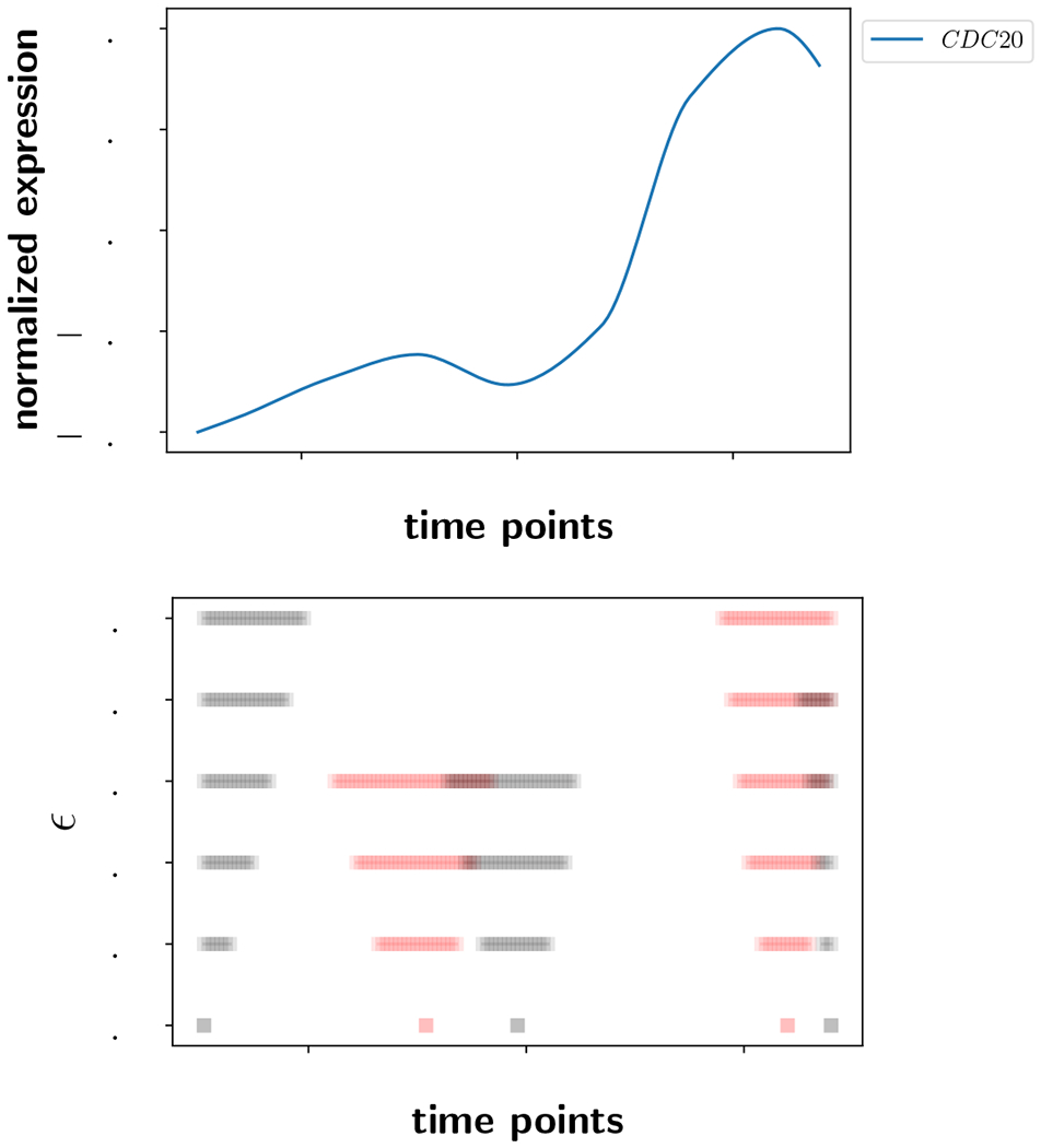
Top: A smoothed and normalized time series. Bottom: The ε-extremal intervals as a function of increasing noise ε. The gray lines correspond to local minima and the reddish lines are associated to local maxima.

The bottom row in the lower plot has five points marked, each of which is an interval of length zero corresponding to the case without noise, ε = 0. At a noise level of ±1%, the intervals have widened but remain distinct. At a noise level of ±2%, some of the intervals have started to overlap. Somewhere between ±3% and ±4%, the two intervals corresponding to the maximum and minimum near time point 100 have widened so much that they coincide. When two intervals coincide, it means the ε-band has become so large that the true time series T₁ is not guaranteed to have any extrema within that interval, and the interval is removed from ${\mathcal{I}}_{\epsilon }(D_1)$. Between ±4% and ±5%, the interval associated to the right endpoint minimum has become a proper subset of the interval of the adjacent maximum. The interval containing the maximum continues to the 5% noise level, while the interval associated to the rightmost minimum has been removed from ${\mathcal{I}}_{\epsilon }(D_1)$. Every time an interval becomes a proper subset of another interval, the smaller interval is removed and the larger one is retained in ${\mathcal{I}}_{\epsilon }(D_1)$. The reason is because the true time series T₁ is only guaranteed to attain the extremum associated to the larger interval.

The top row in the lower plot provides a description of the time series assuming a measurement error of ±5%. At this level of precision, the time series is characterized by a global minimum well-separated from a global maximum. When the noise level increases enough that these last two intervals coincide, which they will do by a 50% noise level, then we say that the time series is ε-constant. At that point in time, all information about the extrema of the time series (if they exist) is is erased by noise.

As alluded to above, the key property that guides the construction of the collection of intervals ${\mathcal{I}}_{\epsilon }(D_i)$ is the following. Let l be the linear interpolation of a time series D_i and let e be its local extremum. For a fixed measurement error level ε, let $I\in {\mathcal{I}}_{\epsilon }(D_i)$ be the ε-extremal interval containing e. We prove in Section 4 that every continuous function whose graph lies within the band l ± ε must attain an extremum of the same type as e (maximum or minimum) within the interval I. Moreover, I is the minimal such interval about e with this property, up to the discretization level of the time series. This means that the intervals ${\mathcal{I}}_{\epsilon }(D_i)$ describe the position of extrema of a time series in a way that is robust to noise in the most precise way possible given the information in the dataset. Naturally, if important extrema are missing from the dataset due to sparse time points, then this method cannot guess at their existence.

Using our approach, a dataset $\mathcal{D}$ is represented as a strict partial order $P_{\epsilon }(\mathcal{D})=({\mathcal{I}}_{\epsilon }(\mathcal{D}),◁)$ of the collection of intervals representing extrema for all time series in the dataset. If $I\in {\mathcal{I}}_{\epsilon }(\mathcal{D})$ is an interval in time series D_i and $J\in {\mathcal{I}}_{\epsilon }(\mathcal{D})$ is an interval in time series D_j with i ≠ j, then I ◁ J if and only if the right endpoint of I is less than or equal to the left endpoint of J. In other words, I is comparable to J if and only if the intervals are disjoint, except possibly at a single point. When intervals are disjoint, then the extrema they represent are well-separated and can be unambiguously distinguished. Since not all pairs of intervals in ${\mathcal{I}}_{\epsilon }(\mathcal{D})$ are comparable, the intervals are only partially ordered.

Each partial order $P_{\epsilon }(\mathcal{D})$ can be represented as a graph $H_{\epsilon }^R(V,E)$, called the Hasse diagram, with nodes V corresponding to intervals in ${\mathcal{I}}_{\epsilon }(\mathcal{D})$, and an edge in E ⊂ V × V whenever I ◁J. This graph is a coarse representation of the information contained in the dataset, containing qualitative rather than quantitative phase shifts.

As ε increases, there are fewer disjoint intervals in ${\mathcal{I}}_{\epsilon }(\mathcal{D})$, fewer well-ordered pairs of intervals, and therefore fewer restrictions on the ordering of extrema between time series. This results in a more permissive partial order, where the amount of trusted information decreases as assumed noise level increases. Eventually, ε increases to the point where some neighboring extrema become indistinguishable and the number of nodes in $H_{\epsilon }^R(V,E)$ decreases. We illustrate this on an example in Figure 2. In the upper left, there are two interpolated and normalized time series. The blue curve is the same as the one in Figure 1 (top), and has five local extrema. The second orange curve has four local extrema including endpoints. We calculate the ε-extremal intervals for both curves for ε = 0.0, 0.03, and 0.05 and get the Hasse diagrams of the partial orders shown in the figure. In every Hasse diagram, the arrow of time points downward.

Figure 2:

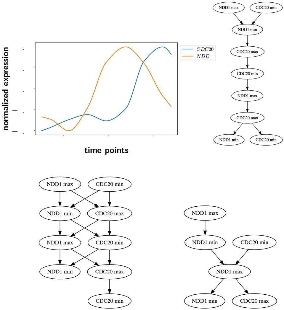
Hasse diagrams of two time series as a function of ε. Upper left: The time series under consideration. Upper right: ε = 0.0. Lower left: ε = 0.03. Lower right: ε = 0.05.

At the upper right in Figure 2 is the Hasse diagram for ε = 0.0, which corresponds to the case without noise, and all nine local extrema are represented. At ε = 0.03 (lower left), all nine extrema are still present, but the greater number of incomparable ε-extremal intervals indicates a more permissive partial order. For example, at ε = 0, the first NDD1 minimum (the one closest to the top of the Hasse diagram) must occur before the first CDC20 maximum. But when ε = 3% those two extrema are incomparable, as indicated by the lack of an arrow between them in the Hasse diagram on the lower left. At the lower right with ε = 5%, there are only six extrema. CDC20 has lost its two middle extrema and its rightmost minimum, as shown in Figure 1 (bottom) where ε = 0.05.

As motivation for the work in Section 4, we discuss the applications of our method after a brief introduction to some standard definitions in graph theory. Application 1 demonstrates that the ε-extremal interval method can be used for consistency-checking a DSGRN model of network dynamics as suggested in [1]. Application 2 shows that the technique can be used to quantify the similarity between different time series datasets.

For the purpose of the presentation of the applications we will ask the reader to accept that the collection ${\mathcal{I}}_{\epsilon }(\mathcal{D})$, the partial order $P_{\epsilon }(\mathcal{D})=({\mathcal{I}}_{\epsilon }(\mathcal{D}),◁)$, and its representation $H_{\epsilon }^R(V,E)$ can be unambiguously constructed for any dataset $\mathcal{D}$ and any ε. Rigorous technical detail for the method of ε-extremal intervals is given in depth in Section 4, along with information on the computational implementation [21]. Section 4 may be read before the applications in Section 3 if desired.

2. Graph theory preliminaries

Definition 1. A directed graph G(V,E) is a set of nodes (or vertices) V, together with a collection of edges E ⊆ V × V. A labeled, directed graph G(V, E, ℓ) has in addition a labeling function ℓ that assigns labels to the nodes and/or edges of a graph.

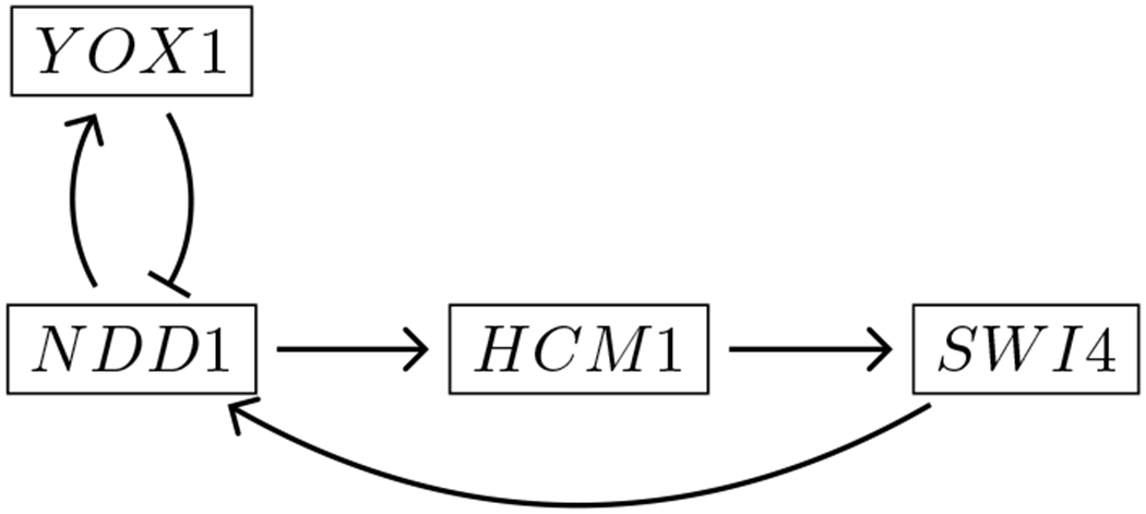
We will refer to all of unlabeled, node-labeled, and node- and edge-labeled graphs in this manuscript. One important example is a gene regulatory network, which is a node- and edge-labeled directed graph. Each node is labeled by the gene product that it represents, and every edge is labeled either as an activating (→) or repressing (⊣) edge. The gene regulatory network that we will explore in Application 1 is shown in Figure 3.

Figure 3:

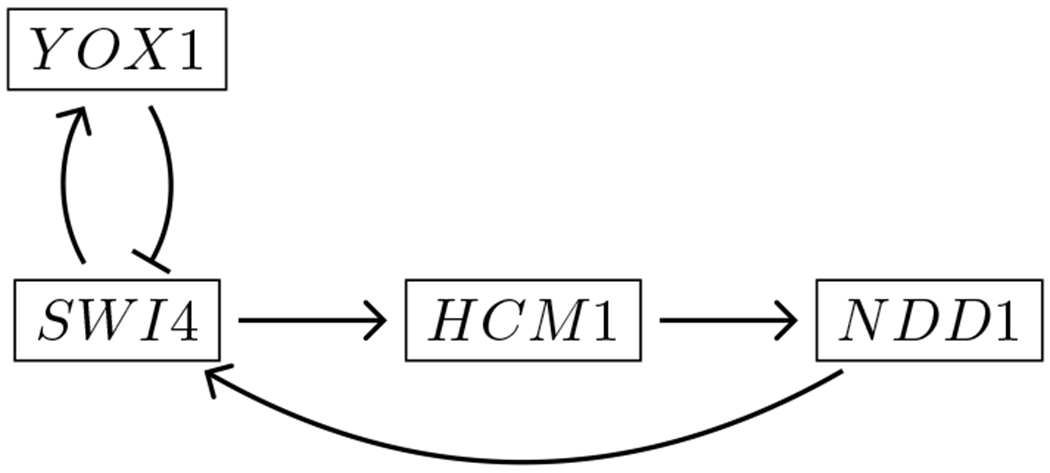
Wavepool model of core genes involved in regulation of the yeast (S. cerevisiae) cell cycle [22].

Definition 2. A partial order P = (S, ≤) is a binary relation ≤ on the set S that is reflexive, antisymmetric, and transitive. A strict partial order P = (S, <) is a binary relation < on the set S that is antisymmetric and transitive. A (strict) total order is a (strict) partial order where for any pair (a, b) ∈ S × S either a ≤ b (a < b) or b ≤ a (b < a). A linear extension of a (strict) partial order is a (strict) total order T such that if a ≤ b (a < b) in P, then a ≤ b (a < b) in T.

In this manuscript, we will only be concerned with strict partial and strict total orders. Our notation reflects this, but for brevity we will often refer only to partial and total orders.

Every partial order can be represented as a directed graph called a Hasse diagram. To explain Hasse diagrams, it is useful to know the concepts of transitive closures and transitive reductions. A transitive closure adds a direct edge wherever there is a path between two nodes, and a transitive reduction removes an edge whenever there is a longer path from one node to another.

Definition 3. Let G(V, E) be a directed graph. A node j is reachable from a node i in the graph G if there exists a path

$$(i,i_1),(i_1,i_2),\dots ,(i_n,j)$$

such that each edge (i_j, i_j+1) ∈ E. The transitive closure of G(V, E) is the directed graph G^C(V, E′) with E ⊆ E′ such that (i, j) ∈ E′ if and only if j is reachable from i in G The transitive reduction of G(V, E) is the directed graph G^R(V, E″) with the minimal set of edges E″ ⊆ E such that if the vertex j ∈ V is reachable from i ∈ V in the graph G, then j is reachable from i in G^R.

Definition 4. Let P = (S, <) be a strict partial order on a finite set S. Let H(V, E) be a directed graph where the nodes V are in a bijection with the elements of the set S, and an edge (i,j) ∈ E if and only if i < j. The Hasse diagram H^R(V, E″) of P is the transitive reduction of H.

Note that the graph H defined in Definition 4 is its own transitive closure, H(V, E) = H^C(V, E), because the partial order P is transitively closed. For clarity, we will refer to H^C rather than H in the text. The Hasse diagram H^R plays a role in both Applications 1 and 2, and the transitive closure of the Hasse diagram H^C is important in Application 2. We will use the notation $H_{\epsilon }^R(\mathcal{D})$ and $H_{\epsilon }^C(\mathcal{D})$ for a given dataset $\mathcal{D}$ and noise level ε.

Every partial order P is associated to a unique distributive lattice. This is the content of Birkhoff’s Representation Theorem (see Chapter 5 in [23]).

Definition 5. Let P = (S, <) be a strict partial order over a finite set S. A down-set is any set Q ⊆ S such that if a ∈ Q and b < a, then b ∈ Q. A down-set lattice is the partial order $P^{\prime }=(\mathcal{O}(P),\subset )$, ordered by set inclusion, where $\mathcal{O}(P)$ is the collection of down-sets of P.

The down-set lattice has a minimal element, the empty set, and a maximal element, S. In the Hasse diagram of the down-set lattice, the two nodes associated to these sets are called the root and the leaf respectively. For brevity, we will use the term down-set lattice interchangeably with the Hasse diagram of the down-set lattice.

Remark 1. The paths from root to leaf in the down-set lattice are in a one-to-one correspondence with the collection of linear extensions of P. This observation plays a central role in Application 1.

Definition 6. A graph distance is a non-negative, real-valued, symmetric function d(G₁, G₂) acting on two graphs G₁ and G₂ that satisfies the triangle inequality and that is zero if and only if G₁ = G₂.

The graph distance described in Section 4.3.3 for node-labeled, directed graphs is used in Application 2 to assess the similarity between two time series datasets.

3. Applications

3.1. Model rejection via pattern matching

3.1.1. DSGRN

In our previous work [12] we introduced a method to describe the global dynamics of a regulatory network for all parameters. This approach, named DSGRN (Dynamic Signatures Generated by Regulatory Networks) [17], uses combinatorial dynamics generated by switching systems [13, 14, 15, 16] to construct a database of all possible dynamics that a network may exhibit.

The core procedure of DSGRN [12, 17] is the following:

1. A switching system ODE model is associated to a gene regulatory network. The dimension of phase space is the number of nodes in the network, N. The dimension of parameter space is 3M + N, where M is the number of edges in the network.

2. The form of switching systems allows parameter space ${\mathbb{R}}_{+}^{3M+N}$ to be decomposed into a finite number of semi-algebraic regions. We call each region a DSGRN parameter.

3. The form of switching systems also admits a decomposition of phase space ${\mathbb{R}}_{+}^N$ into a finite number of rectangular regions (boxes). The number of boxes depends on the number of discrete states that each gene product can attain, which is exactly one more than the number of out-edges from the corresponding node.

4. The dynamics of the switching system for a DSGRN parameter are captured by a state transition graph, in which each node is associated to one of the boxes in phase space, and edges capture the direction of the normal component of the vector field at a boundary between two boxes. This assignment is consistent if there is no negative self-regulation in the regulatory network [14]. A solution trajectory of the switching system then corresponds to a path in the state transition graph.

DSGRN produces a finite collection of state transition graphs that captures the parameter dependence of the dynamics across all of parameter space.

Important to the application here, the nodes of the state transition graph can be labeled by whether each gene product is increasing (I), decreasing (D), or both (*) in the corresponding phase space box. Likewise, the edges can be labeled by which variable is attaining an extremum between boxes (M for maximum, m for minimum, a dash for neither). By assumptions on the switching system, only one gene product may attain an extremum at a time. An example labeled state transition graph for a fixed DSGRN parameter for the network in Figure 3 is shown in Figure 4.

Figure 4:

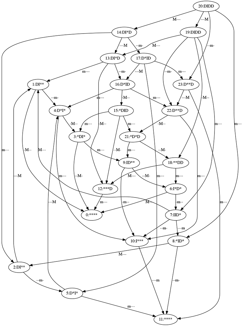
Example state transition graph for the network in Figure 3. This is a state transition graph as described in the text, with 4-symbol labels indicating whether a variable is increasing (I), decreasing (D), or both (*) in the corresponding partition of phase space. The order of the symbols is SWI4, HCM1, NDD1, and YOX1. The edge labels indicate the possibility of a local maximum (M) or minimum (m) for each variable. The dash indicates that no extremum is possible for that variable.

3.1.2. DSGRN model consistency with a dataset

In a recent paper [1], we compared a DSGRN model of molecular regulation to experimentally observed time series. We proposed that a network can be rejected as a model of a biological system that produces the experimental dataset D if there is no DSGRN parameter at which a path in a DSGRN state transition graph is “consistent” with the partial order $P_{\epsilon }(\mathcal{D})$ derived from a dataset.

A path is consistent with partial order $P_{\epsilon }(\mathcal{D})$ if it is a linear extension of $P_{\epsilon }(\mathcal{D})$. Any linear extension of $P_{\epsilon }(\mathcal{D})$ is a total order of the extrema consistent with the time discretization and the measurement error level ε. Therefore a path in the state transition graph that is a linear extension of $P_{\epsilon }(\mathcal{D})$ represents a solution trajectory that has an order of extrema consistent with noise level ε in the data. If such an extension exists, the network cannot be rejected as a valid model.

Because we are seeking a linear extension, we make use of the down-set lattice structure introduced in Definition 5, since it is a summary of all linear extensions of $P_{\epsilon }(\mathcal{D})$. First, the lattice is augmented with labels. In the Hasse diagram of $P_{\epsilon }(\mathcal{D})$, $H_{\epsilon }^R(\mathcal{D})$ the nodes can be naturally labeled with extrema. Therefore one can unambiguously label the edges of $H_{\epsilon }^R(\mathcal{D})$ based on whether the gene product is increasing or decreasing, which is opposite to the labeling on the state transition graph. We showed that there is a natural way to assign dual labeling to the down-set lattice. In other words, the lattice can be labeled unambiguously with extrema on the edges and increasing or decreasing behavior on the nodes. Second, the lattice is augmented with self-edges at every node. Since gene products may monotonically increase or decrease in concentration across multiple boxes before reaching an extremum, self-loops were added to represent this dwell time. The resulting graph is called a pattern graph, and has a unique root node and a unique leaf node. An example is shown in Figure 6 based on the time series introduced in Figure 5.

Figure 6:

Corresponding pattern graph for $H_{0.15}^R(\mathcal{D})$ in Figure 5 (lower right). The 4-symbol node labels with I (increasing) and D (decreasing) and the edge labels with m (minimum) and M (maximum) symbols have the same meaning as in Figure 4. Notice the unique root and unique leaf.

Figure 5:

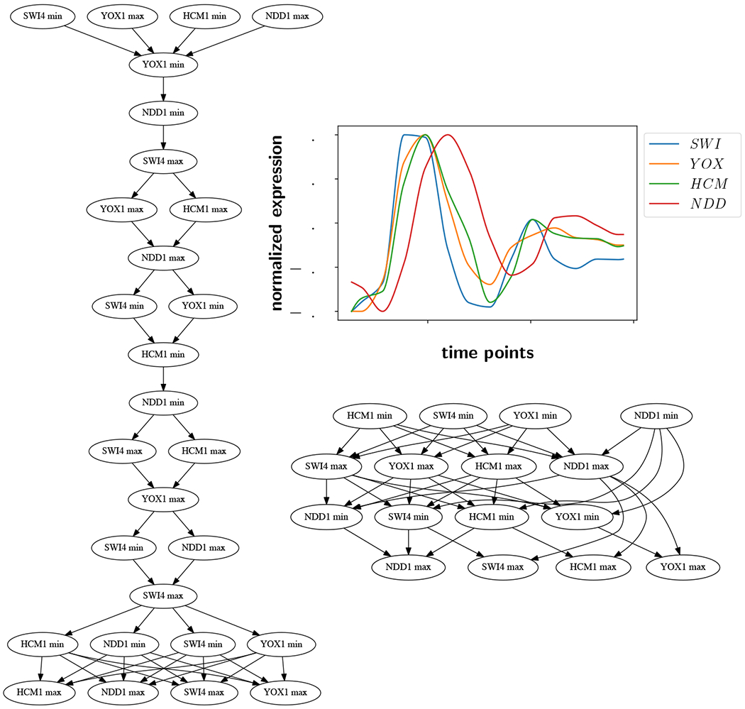
S. cerevisiae time series data [28] (upper right) and example $H_{\epsilon }^R(\mathcal{D})$ for the data at ε = 0.0 (left) and ε = 0.15 (lower right). The arrow of time points downward on the Hasse diagrams.

We seek a pair of paths with matching labels on both nodes and edges, where one path goes from root to leaf in the pattern graph and the other path is in the state transition graph. The matching relation between labels that we define allows for non-exact matches; namely the symbol * is allowed to match both I and D. This is a type of approximate graph matching [24, 25, 26, 27]. If such a pair exists, then the model is consistent with the data and cannot be rejected. In [1], we formulate this consistency problem as a graph theory problem with a polynomial time algorithm.

In Figure 5 of [1], the partial order $P_{\epsilon }(\mathcal{D})$ was calculated by hand via visual inspection of the data. We illustrate the approach developed in this paper on the example from [1].

3.1.3. Cell cycle data model

In Figure 5 (upper right), we present microarray time series data from the yeast S. cerevisiae, which was normalized between −0.5 and 0.5. The data were published in [28], and have here undergone shifting via CLOCCS analysis [29] and smoothing via polynomial splines, as described in Appendix A. These data are similar to those in [1] (Section 4.2, data published in [30]), which are data collected on the same genes from the same organism in the same lab, but using RNAseq technology rather than the microarray platform.

We show two partial orders arising from this data at two noise levels using the ε-extremal interval method. The Hasse diagrams are shown in Figure 5 at ε = 0.0 (left) and 0.15 (lower right). The number of extrema at a noise level of 0 is 28, and drops to 16 at a noise level of 0.15. The partial order at ε = 0.0 is far more restrictive (and thus looks closer to a total order), because few of the intervals overlap, and more order relations are known. The pattern graph associated to the partial order on the right is shown in Figure 6.

The regulatory network in Figure 3 is a simplified version of the wavepool model, introduced in [22]. This model has been corroborated experimentally [31, 32, 33] and describes the mechanism for controlling the cell-cycle transcriptional program.

In [1], we verified that the wavepool model is consistent with the data. We find the same result here. In particular, there is a pair of matching paths between Figures 4 and 6 of length 17:

$$\begin{gathered} (18,38)\to (6,37)\to (7,34)\to (8,32)\to (2,31)\to (5,42)\to (4,25)\to (3,22) \\ \to (9,21)\to (6,19)\to (7,65)\to (8,63)\to (2,13)\to (5,80)\to (4,7) \\ \to (3,4)\to (0,0) \end{gathered}$$

The first number is the integer node label in Figure 4, and the second is the integer node label in Figure 6. The first node pair is at the root of the pattern graph (node 38) and the last node pair is at the leaf of the pattern graph (node 0). It can be verified that the labels at each pair of nodes match, remembering that the wild card character * matches itself, I, and D. Likewise, the edge labels match as well. So at the DSGRN parameter that produced the state transition graph in Figure 4, the wavepool network model cannot be rejected.

3.1.4. Global assessment of the network model

We seek to characterize the performance of the wavepool model across parameter space and across various levels of noise. Recall that we use the variable ε to denote a band of noise around a time series. Recall also that the partial order representing the dataset $P_{\epsilon }(\mathcal{D})$ depends on ε, so that the pattern graph depends on ε as well. We independently normalized each time series in the dataset between −0.5 and 0.5 so that ε represents a percentage of the distance between the global maximum and global minimum of each time series in the dataset.

The wavepool network in Figure 3 has 1080 DSGRN parameters. For ε values ranging from 0.0 to 0.15, we searched for pairs of matching paths between the pattern graph and the state transition graph at each DSGRN parameter using the DSGRN pattern matching algorithm described in [1] and implemented in [17]. See Figure 5 for the partial orders $P_{0.0}(\mathcal{D})$ and $P_{0.15}(\mathcal{D})$ showing the extremes of the representation of the dataset.

The results are summarized in the first row of Table 1. There are 22 DSGRN parameters in the wavepool network that exhibit consistent dynamics with the time series in Figure 5 (upper right) for noise levels ε = 0.01 through 0.04. This is the same number of DSGRN parameters with path matches found in [1].

Table 1:

Number of parameters with at least one match to $P_{\epsilon }(\mathcal{D})$.

ε	0.0	0.01	0.04	0.05	0.06	0.08	0.09	0.10	0.14	0.15
Figure 3	0	22	22	12	12	42	24	24	24	24
Figure 7	0	0	0	0	0	0	0	0	22	22

Although the number of matches is the same, none of the partial orders $P_{\epsilon }(\mathcal{D})$ match the one computed by hand in [1]. This is likely due to the difference in sampling times; the RNAseq data in [1] have a sampling interval of 5 minutes, while the microarray data have a sampling interval of 16 minutes. This discrepancy can be responsible for different resolutions in peak detection, and therefore change the representative partial orders. It is also possible that the CLOCCS shifting of the microarray dataset resulted in a small phase shift with respect to the RNAseq data, which could alter the relative locations of the extrema.

In addition to the difference in partial orders, we also do not know if the collection of parameters at which there are pattern matches is the same between this work and the previous one. However, the fact that the model has comparable performance under different data collection platforms and sampling intervals highlights both the reproducibility of the performance of the S. cerevisiae cell cycle, and the power of this technique to identify/reject models based on time series data.

We note that at ε = 0, the wavepool model has no matches to the partial order in Figure 5 (left). Without considering noise, we would be tempted to reject the hypothesis that the wavepool model is consistent with the experimental data.

However, the ability to scan through different potential noise levels reveals that the wavepool model cannot be rejected, as it consistently matches the data over a range of small noise levels.

Finally, we observe that the number of matches does not increase monotonically with ε. This may at first seem counterintuitive, since as intervals grow larger and overlap, the number of constraints in the partial order is reduced. However, nodes in the graph representing shallow extrema in the time series disappear as ε grows larger, which changes the size of the graph. Under these conditions, there is no guarantee of monotonicity. In our example here, the number of nodes in the partial order decreases from 28 to 16 as ε increases from 0 to 0.15. At ε = 0.08, we find the highest number of parameters with matches, 42.

3.1.5. Model rejection

In a second numerical experiment, we propose a different model for the same time series data, depicted in Figure 7. Here we swapped the positions of the genes NDD1 and SWI4 compared with the first model, thus creating an “incorrect” model for the data. In [1], no matches were found for this model using the partial order computed by hand and shown in Figure 5 of that work. The number of matches that we find now for this network are shown in second row of Table 1. We observe that there are no matches in this network until noise level ε = 0.14, so that we match [1] in the range ε = 0.01 through 0.04 as before. At a noise level of ε = 0.14, the band of uncertainty around the data is 28% of the difference between the global maximum and the global minimum in the normalized data. This a very high level of noise, and we hypothesize that the partial order at this noise level does not sufficiently constrain the model, leading to matches with models that are inconsistent with experimental results. The large range of noise levels with zero matches would lead us to reject the network in Figure 7 as a description of the biological mechanism that produced the time series data.

Figure 7:

A model in which two genes of the wavepool model are swapped, which our methodology invalidates.

3.2. Quantifying similarity between replicate experiments

In this application, we seek to quantify the similarity between two replicates of the same experiment with datasets ${\mathcal{D}}_1$ and ${\mathcal{D}}_2$. We construct for each dataset partially ordered sets of ε-extremal intervals $P_{\epsilon }({\mathcal{D}}_1)$ and $P_{\epsilon }({\mathcal{D}}_2)$, and represent them by the transitive closures of Hasse diagrams $H_{\epsilon }^C({\mathcal{D}}_1)$ and $H_{\epsilon }^C({\mathcal{D}}_2)$ as in Definitions 3 and 4. We then calculate a graph distance between $H_{\epsilon }^C({\mathcal{D}}_1)$ and $H_{\epsilon }^C({\mathcal{D}}_2)$, which is roughly the proportion of non-shared edges between the two graphs; see Section 4.3.3 for a precise definition. The distance $d(H_{\epsilon }^C({\mathcal{D}}_1),H_{\epsilon }^C({\mathcal{D}}_2))$ that we use is scaled so it has a range between 0 and 1. We say that the similarity between two datasets ${\mathcal{D}}_1$ and ${\mathcal{D}}_2$ is given by

$$s({\mathcal{D}}_1,{\mathcal{D}}_2)=1-d(H_{\epsilon }^C({\mathcal{D}}_1),H_{\epsilon }^C({\mathcal{D}}_2)).$$

This similarity measure gives roughly the proportion of shared edges between $H_{\epsilon }^C({\mathcal{D}}_1)$ and $H_{\epsilon }^C({\mathcal{D}}_2)$.

In order for the comparison of the two datasets to be biologically relevant, they must be synchronized at the same point in the yeast cell cycle. In the datasets we consider, the time series were processed to align with the yeast cell cycle using the techniques described in Appendix A. After this processing, we normalized the data to the range [−0.5, 0.5] and truncated so that most of the time series exhibited one period, as shown in Figure 8. The truncation limits the computation time of the graph distance, and focuses the analysis on the highest and most synchronized peaks.

Figure 8:

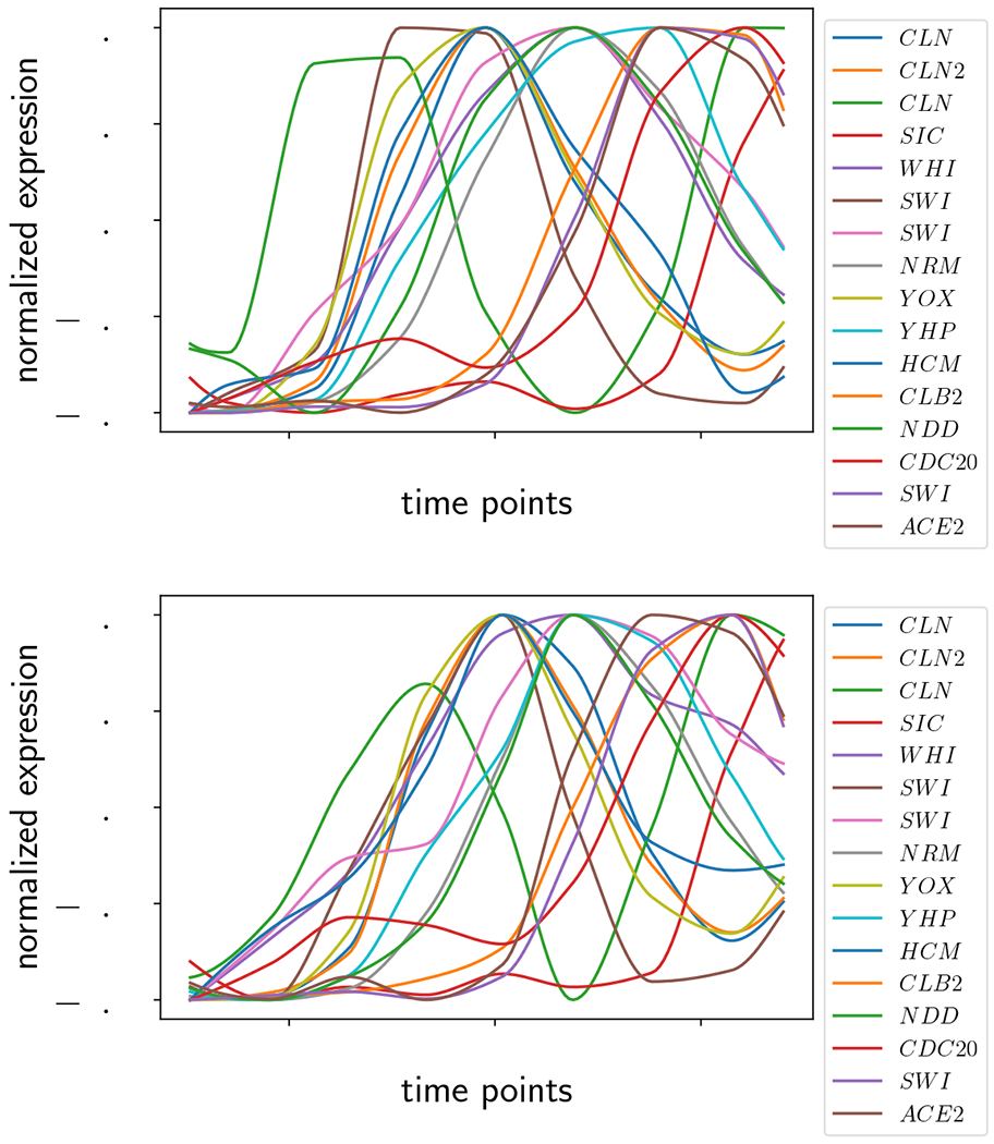
Microarray yeast cell cycle data from [28], processed as described in Appendix A. (Top) Replicate 1. (Bottom) Replicate 2.

To illustrate the properties of the similarity measure, we perform four different comparison experiments.

1. We first concentrate on only four genes, SWI4, YOX1, NDD1, and HCM1. We denote by ${\mathcal{D}}_1^{\prime }$ and ${\mathcal{D}}_2^{\prime }$ the time series of these four genes extracted from experiments ${\mathcal{D}}_1$ and ${\mathcal{D}}_2$, respectively (see Figure 9 top row). We calculate the similarity $s({\mathcal{D}}_1^{\prime },{\mathcal{D}}_2^{\prime })$ over a range of ε.

2. We compute $s({\mathcal{D}}_1^{\prime },{\mathcal{D}}_2^{″})$, where ${\mathcal{D}}_2^{″}$ is the dataset formed by time series SWI4, CLB2, NDD1, and HCM1. Here we replace the time series of YOX1 in the second dataset by the time series of CLB2, where the CLB2 time series can be seen in Figure 8.

3. We compare the same data as in (2), but we mislabel CLB2 in ${\mathcal{D}}_2^{″}$ as YOX1. We call the mislabeled dataset ${\mathcal{D}}_3^{″}$. The calculation of $s({\mathcal{D}}_1^{\prime },{\mathcal{D}}_3^{″})$ shows the effect of replacing the YOX1 data in ${\mathcal{D}}_2^{\prime }$ by a different time series. The comparison between experiments (2) and (3) gives an idea of the impact on the distance measure when there are non-matching gene labels in the partial orders.

4. Lastly, we compare all of the time series by randomly sampling four genes to construct datasets ${\widehat{\mathcal{D}}}_1$ and ${\widehat{\mathcal{D}}}_2$ one hundred times, and calculating $s({\widehat{D}}_1,{\widehat{D}}_2)$ for each over a range of ε. The mean of these curves is taken to be representative of the full dataset. The same experiment is performed with random samples of eight genes to show the dependence of results on gene sample size.

Figure 9:

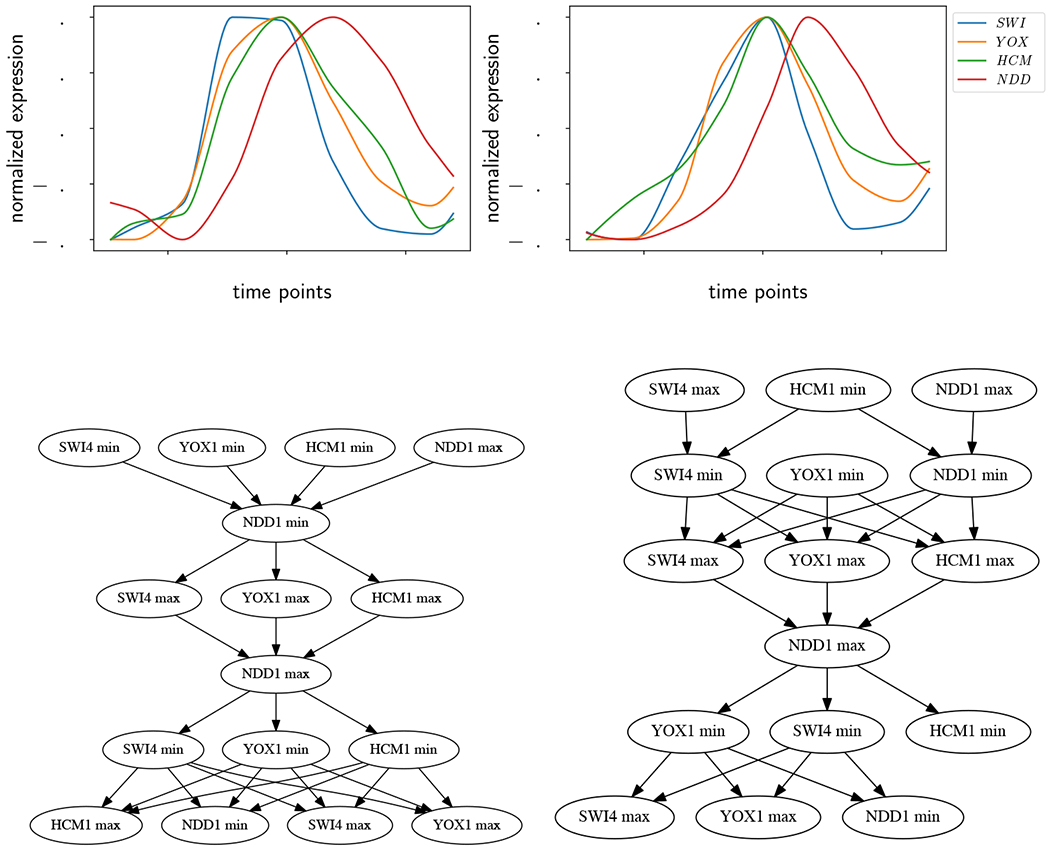
(Top left) Time series for replicate 1. (Top right) Time series for replicate 2. (Bottom left) Hasse diagram $H_{0.01}^R({\mathcal{D}}_1^{\prime })$ for replicate 1 at ε = 0.01. (Bottom right) Hasse diagram $H_{0.01}^R({\mathcal{D}}_2^{\prime })$ for replicate 2 at ε = 0.01. The arrow of time points downward on the Hasse diagrams.

Experiment 1:

We compute ε-extremal intervals to produce a partially ordered set of extrema for ${\mathcal{D}}_1^{\prime }$ and ${\mathcal{D}}_2^{\prime }$. As an example, the Hasse diagrams $H_{0.01}^R({\mathcal{D}}_1^{\prime })$ and $H_{0.01}^R({\mathcal{D}}_2^{\prime })$ for ε = 0.01 are shown in the bottom row of Figure 9. Although we use the transitive closure $H_{\epsilon }^C(\mathcal{D})$ to calculate distances, the transitive reductions are shown for simplicity, so that the structures of the partial orders are easier to compare.

We repeat this procedure at noise levels ε = 0 to 0.15 at intervals of 0.005. The similarity $s({\mathcal{D}}_1^{\prime },{\mathcal{D}}_2^{\prime })$ was calculated at each ε and represented as the blue curve in Figure 10. Notice that the similarity between the partially ordered sets goes to 1 at larger values of ε and varies between 0.7 and 1.0 over the whole range of ε. To assess if this represents strong or weak similarity, we perform two other numerical experiments.

Figure 10:

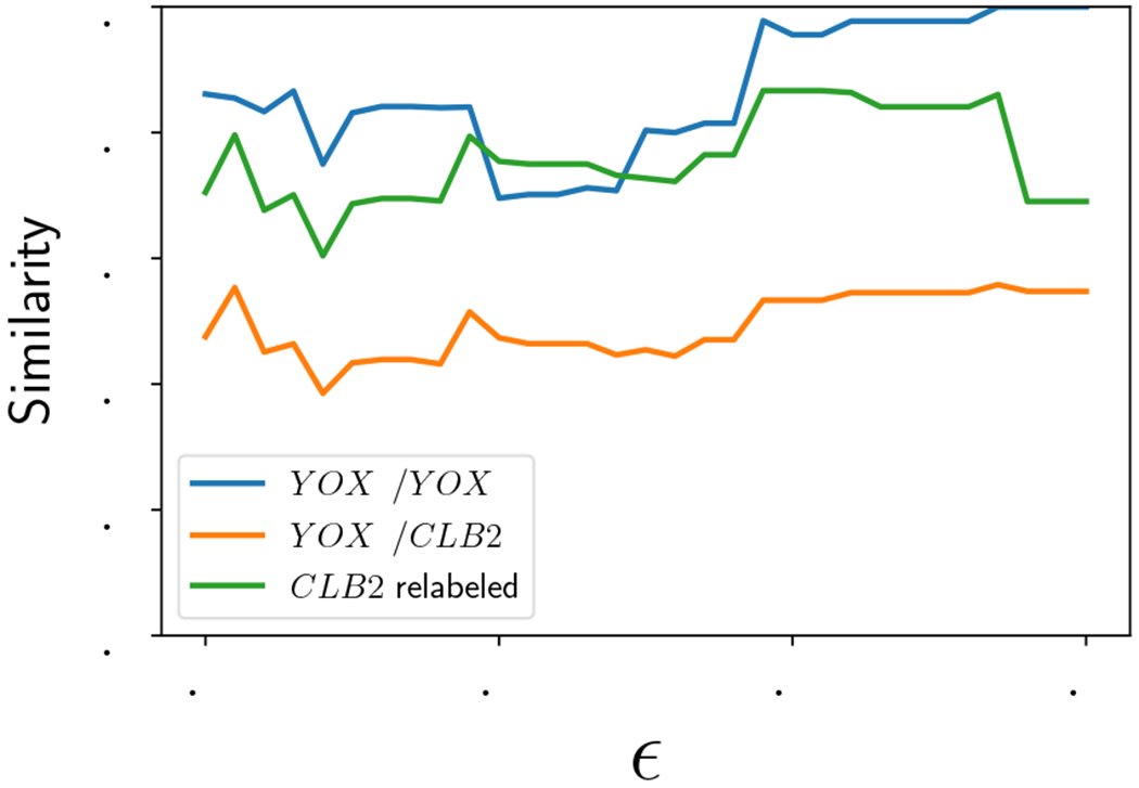
Similarity as a function of ε. Blue curve: Experiment 1, $s({\mathcal{D}}_1^{\prime },{\mathcal{D}}_2^{\prime })$. Orange curve: Experiment 2, $s({\mathcal{D}}_1^{\prime },{\mathcal{D}}_2^{″})$. Green curve: Experiment 3, $s({\mathcal{D}}_1^{\prime },{\mathcal{D}}_3^{″})$.

Experiment 2:

We replace the second data set ${\mathcal{D}}_2^{\prime }$ by the dataset ${\mathcal{D}}_2^{″}$ composed of genes SWI4, CLB2, NDD1, and HCM1, and we show the similarity $s({\mathcal{D}}_1^{\prime },{\mathcal{D}}_2^{″})$ in the orange curve in Figure 10. Since the YOX1 extrema in replicate 1 are being compared with the CLB2 extrema in replicate 2, the distance between the partially ordered sets is larger than in Experiment 1. The similarity between the partial orders ranges between about 40-55%. This gives an idea of the distance when nodes cannot be matched across partial orders because of a single time series swap.

Experiment 3:

We relabeled all “CLB2” extrema in replicate 2 to “YOX1” labels to get dataset ${\mathcal{D}}_3^{″}$. This allows us to compare the distance when the curve shape of CLB2 is used in place of the true YOX1 data. The resulting similarities $s({\mathcal{D}}_1^{\prime },{\mathcal{D}}_3^{″})$ are shown in the green curve in Figure 10. By comparing the orange curve (Experiment 2) with the green curve (Experiment 3) in Figure 10, it can be seen that having mismatched labels contributes substantially to the dissimilarity of time series. However, even when the mismatched labels are artificially removed with relabeling, we see by comparing the blue curve (Experiment 1) with the green curve (Experiment 3) in Figure 10 that using the same set of time series in both replicates leads to a noticeably higher similarity over most of the range of ε.

Experiment 4:

We now consider all the time series in the dataset, as shown in Figure 8, to quantify the similarity of the two replicates as a function of noise. Because our algorithm for graph distance does not scale favorably with the size of the graph, we chose to (a) sample ε more coarsely from 0 to 0.15 at intervals of 0.01, and (b) pick at random one hundred samples of four and eight genes each, and then calculate the mean similarity. The resulting curves are shown in Figure 11 with samples of 4 genes on the left and 8 genes on the right. The thick black line indicates the mean and ±1 standard deviation of the one hundred samples shown in grey. The mean on both curves ranges between about 75-95% similarity, with the bulk of the values over 80% similar. The standard deviation decreases substantially with increasing gene sample sizes, suggesting that sampling subsets of genes is a reasonable proxy for calculating the similarity of the whole dataset.

Figure 11:

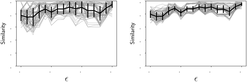
Similarity $s({\widehat{\mathcal{D}}}_1,{\widehat{\mathcal{D}}}_2)$ as a function of ε. Thin gray curves: one hundred samples of 4 genes each (left) and 8 genes each (right) from the 16 genes listed in the legend of Figure 8. Thick black curve: Mean of the one hundred samples with ±1 standard deviation.

4. Methods

The applications in the previous section are dependent on the representation of a time series dataset $\mathcal{D}$ by a partial order $P_{\epsilon }(\mathcal{D})$ over time intervals ${\mathcal{I}}_{\epsilon }(\mathcal{D})$ representing the location of extrema up to a noise level ε. We now present in detail the construction of the intervals ${\mathcal{I}}_{\epsilon }(\mathcal{D})$.

We begin in Section 4.1 by establishing the theory for continuous functions. For $f:[x_1,x_2]\to \mathbb{R}$ a continuous function on a closed interval [x₁, x₂], we present an approach that finds a collection of intervals ${\mathcal{J}}_{\epsilon }(f)$, called ε-extremal intervals, with the property that any continuous function g whose values are within measurement error ε of f is guaranteed in each interval $I\in {\mathcal{J}}_{\epsilon }(f)$ to attain a local extremum.

Our main tool is the notion of the merge tree of f [18, 19] that we use to define a new object, called the normalized branch decomposition of f on [x₁, x₂]. The normalized branch decomposition allows us construct a collection of ε-minimal intervals on [x₁, x₂], such that every continuous function g that remains within the bounds f − ε and f + ε is guaranteed to achieve a minimum in each ε-minimal interval. By taking −f and applying the same method, we construct ε-maximal intervals, in which every perturbation g of f bounded by ε is guaranteed to attain a local maximum. The union of ε-minimal and ε-maximal intervals forms the set ${\mathcal{J}}_{\epsilon }(f)$.

The extension of merge trees and branch decompositions to discrete time series is straightforward [34]. We show in Section 4.2 that ε-extremal intervals ${\mathcal{I}}_{\epsilon }$ can also be assigned to a discrete time series by using the linear interpolation to construct a continuous function f. With this view, most of the same theorems hold for discrete time series as for general continuous functions.

In both discrete and continuous cases, there is a total order on the ε-extremal intervals for a single function f. In other words, the ε-extremal intervals represent a sequence of extrema of f that can be trusted up to measurement error level of ε. The total orders associated to a collection of functions {f_i} derived from a time series dataset can be extended to a partial order on the extrema of {f_i}.

In Section 4.3, we discuss Algorithms 1 and 2 of [34] that are used to compute merge trees and branch decompositions for a set of time series. We also discuss algorithms derived from Section 4.2 for constructing ε-extremal intervals, partial orders, and a graph distance for partial orders. We provide a repository [21] in Python 3.7 that implements all the algorithms.

4.1. ε-extremal intervals for continuous functions

Consider a continuous function, $f:[x_1,x_2]\to \mathbb{R}$, defined on a closed interval, $[x_1,x_2]\subset \mathbb{R}$.

Definition 7. Let C([x₁, x₂]) denote the space of continuous functions $g:[x_1,x_2]\to \mathbb{R}$, endowed with the supremum norm. For ε ≥ 0, define

$$N_{\epsilon }(f)≔\{g\in C([x_1,x_2]):\mid f-g\mid <\epsilon \}$$

to be the ε-neighborhood of f. A function g ∈ N_ε(f) will be called an ε-perturbation of f.

Given ε ≥ 0, we would like to compute a collection of intervals, ${\mathcal{J}}_{\epsilon }(f)≔\{I_i^{\epsilon }\}$, $I_i^{\epsilon }\subset [x_1,x_2]$, not necessarily disjoint such that

1. every g ∈ N_ε(f) attains either a minimum or a maximum in each $I_i^{\epsilon }$, and

2. for any nonempty $J\subset I_i^{\epsilon }$, there exists some h ∈ N_ε(f) such that h does not attain a maximum or a minimum in J.

The collection ${\mathcal{J}}_{\epsilon }(f)$ represents a set of extrema corresponding to a noise level of ε.

To construct ${\mathcal{J}}_{\epsilon }(f)$ for all ε, we use merge trees [18, 20, 19, 35] to construct an associated object, which we call the normalized branch decomposition. We will show that the normalized branch decomposition provides the proper framework to allow us to associate a collection ${\mathcal{J}}_{\epsilon }(f)$ to all ε > 0.

4.1.1. Merge trees

The merge tree of a real-valued function, f, captures the connectivity of the sublevel sets, f⁻¹(−∞, h], for each $h\in \mathbb{R}$, similar to how the Reeb graph [18] captures the connectivity of the level sets of a function. Here, we recall the definition of the merge tree associated to a function, and refer the reader to [18] and [19] for more details.

Definition 8. The merge tree of f, denoted T_f, is defined to be the quotient space

$$T_f≔\Gamma (f)∕~,$$

where Γ(f) denotes the graph of f, and for x,y ∈ Γ(f), we declare x ~ y if there exists an $h\in \mathbb{R}$ such that both x and y belong to the same level set of f, f⁻¹(h), and also to the same connected component of the sublevel set, f⁻¹(−∞, h].

See Figure 12 (b) for an example of a merge tree. To visualize the construction of the merge tree, imagine a horizontal line sweeping upward from the bottom of the time series depicted in Figure 14 (a). An intersection of such a line with a local minimum corresponds to a leaf of a merge tree, where the leaves are located at the bottom of the merge tree, and an intersection with a local maximum corresponds to an internal node of the merge tree. Notice that each node of T_f, whether maximum or minimum, is associated to a time at which the extremum is located, t_i, and a height of the extremum, f(t_i). Denote by {ℓ_i} the leaves and by {m_i} the internal nodes of the merge tree. For ℓ_i a leaf, denote its height by a_i = f(t_i), and similarly for m_i an internal node, b_i = f(t_i).

Figure 12:

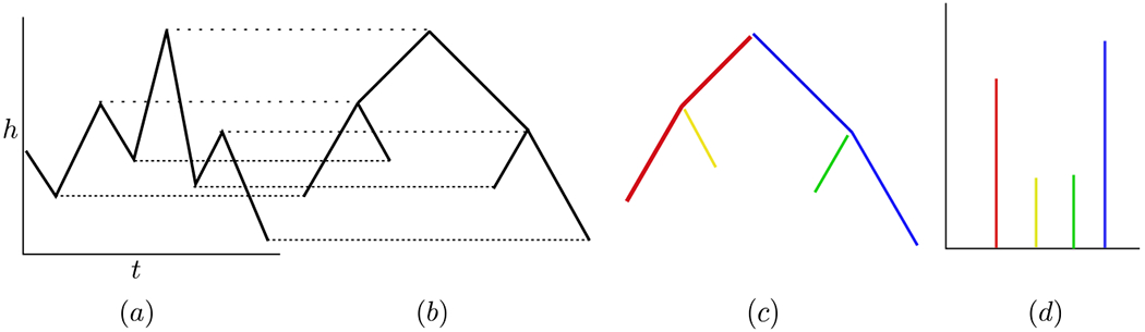
(a) The graph of a function with height h vs time t, (b) its corresponding merge tree, (c) the branch decomposition represented as a colored graph, and (d) the normalized branch decomposition.

Figure 14:

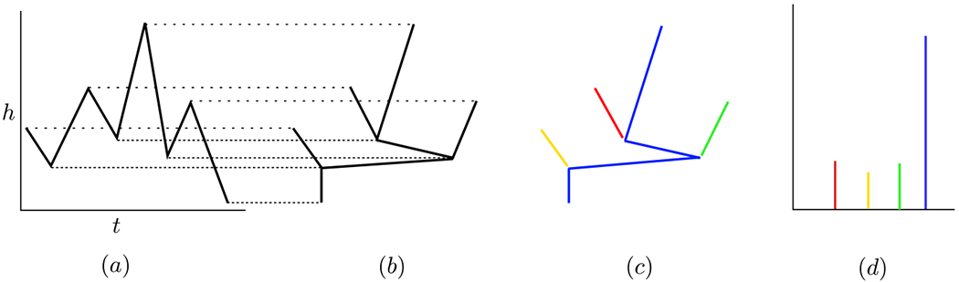
From left to right: the graph of a function, its corresponding dual merge tree, the dual branch decomposition, and the normalized dual branch decomposition.

Note that while the left hand endpoint in Figure 1 (a) is a local maximum, it does not play an important role in the merge tree, Figure 1 (b), because no new topological features appear or merge with other features at that height. The endpoints are the only extrema that might not play a significant role in the merge tree.

4.1.2. Normalized branch decomposition

A branch decomposition is a way of partitioning a merge tree that pairs up the appearance (i.e. birth) and the disappearance (i.e. death) of minima as a function of sublevel height h [20]. The birth heights are given by values {f(t_i)} associated to leaves ℓ_i and the death heights {f(t_k)} correspond to the internal nodes of the merge tree. At each internal node, at least two branches merge. We choose to continue the branch with lowest birth height and terminate all other branches.

This is unambiguous when the branches start at distinct heights. Although having distinct minima is a generic property in continuous functions, experimental time series may be measured only up to some finite resolution, in which case equal height values at which different minima appear may be common. Therefore, in the case that the branches do not start at distinct heights, we arbitrarily decide to continue the branch with the lowest height that also occurs first in time. Other choices are reasonable and would induce different branch decompositions.

Definition 9. We define a total order ≺ on the leaves of the merge tree {ℓ_i} by saying ℓ_i ≺ ℓ_j if one of the following holds:

1. a_i < a_j, or

2. a_i = a_j and t_i < t_j.

This defines an indexing on the leaves of T_f that satisfies ℓ_i ≺ ℓ_i+1 for all i, starting at i = 0.

Definition 10. Let m_k be an internal node of T_f, with associated height b_k. Define S_mk to be the subtree of T_f that is rooted at m_k. We define the branch decomposition of f to be the collection of intervals

1. [a₀, b₀], where b₀ is the global maximum of f; and

2. [a_i,b_k) whenever S_mk is the largest subtree satisfying

   1. ℓ_i is in the subtree S_mk and
   2. ℓ_i ≺ ℓ_j for all ℓ_j ∈ S_mk with i ≠ j.

The branch decomposition can be viewed as a partition of the merge tree, as shown in Figure 12 (c).

Definition 11. The normalized branch decomposition of $f:[x_1,x_2]\to \mathbb{R}$ is a collection of intervals

$$\mathcal{B}(f)≔\underset{i}{⨆}{J}_i,$$

where ⨆ denotes disjoint union, J₀ := [0, b₀ − a₀], and J_i := [0, b_k − a_i) for i > 0 are defined using the branch decomposition of f. Recall that each J_i is uniquely associated to a leaf ℓ_i, with value a_i = f(t_i), and its time of occurrence t_i. We say that t_i is the representative of J_i.

Note that by representing the collection (J_i) as disjoint intervals, we can visualize the normalized branch decomposition as a “barcode”-like summary, which we show in Figure 12 (d).

4.1.3. ε-minimal intervals

We now establish properties of the normalized branch decomposition that allow us to associate a collection of intervals ${\mathcal{J}}_{\epsilon }(f)$ to each parameter ε. First, we describe how to obtain the intervals corresponding to local minima, and then we dualize this procedure to obtain intervals corresponding to the local maxima.

Definition 12. Fix ε > 0. Let $B_{\epsilon }\subset \mathcal{B}(f)$ be the collection of all intervals in the normalized branch decomposition $\mathcal{B}(f)$ that are longer than 2ε,

$$B_{\epsilon }=\{J_i\in \mathcal{B}(f):\mid J_i\mid >2\epsilon \}.$$

Let J_i = [0, b_k − a_i) ∈ B_ε and consider its representative t_i. Define φ(J_i) to be the connected component of (f−ε)⁻¹(−∞, a_i + ε) that contains t_i. Clearly, φ(J_i) is a well-defined relatively open interval in [x₁, x₂]. We define the collection of ε-minimal intervals, denoted

$${\mathcal{J}}_{\epsilon }^{\mathit{min}}\left(f\right):=\left\{\phi \left(J_i\right)|J_i\in B_{\epsilon }\right\}$$

to be the collection of all such intervals. For I_i = φ(J_i), we say that t_i is the representative of I_i as well as of J_i.

See Figure 13 for a depiction of the action of φ. The following Proposition shows that we cannot have overlapping ε-minimal intervals.

Figure 13:

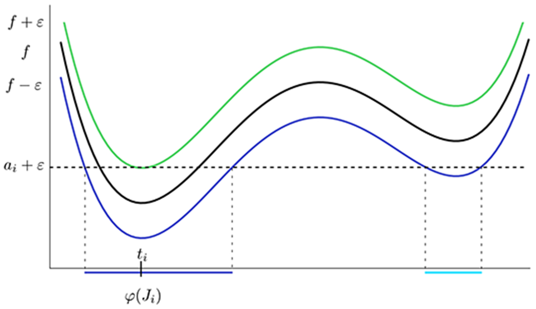
A graph of a function, f, as well as f ± ε. While (f − ε)⁻¹(−∞, a_i + ε) consists of both the dark blue and light blue intervals, φ(J_i) is just the connected component that contains the representative, t_i.

Proposition 1. For any $I_i,I_j\in {\mathcal{J}}_{\epsilon }^{\min }(f)$, I_i ∩ I_j = ∅.

Proof. Consider I_i = φ(J_i) for some J_i = [0, b_k − a_i) ∈ B_ε, and I_j = φ(J_j) for some J_j = [0, b_ℓ − a_j) ∈ B_ε, their representatives t_i and t_j, and their leaves in the merge tree ℓ_i and ℓ_j, respectively. Since t_i and t_j are locations of minima of the continuous function f, there must exist at least one maximum of f between t_i and t_j. Let b_q denote the highest local maximum between the two minima, with location t_q ∈ (t_i,t_j). Notice that if b_q < b_k or b_q < b_ℓ, then the two leaves ℓ_i and ℓ_j are in the same subtree rooted at one of the internal nodes m_k or m_ℓ associated to b_k and b_ℓ respectively. This contradicts the fact that I_i,I_j correspond to distinct branches in the branch decomposition. So b_q ≥ b_k and b_q ≥ b_ℓ. Then by Definition 12,

$$b_q-a_i\ge b_k-a_i>2\epsilon \text{and}{b}_q-a_j\ge b_{\ell }-a_j>2\epsilon ,$$

so that t_q ∉ (f − ε)⁻¹(−∞, a_i + ε) = I_i and t_q ∉ (f − ε)⁻¹(−∞, a_j + ε) = I_j. Since t_q ∈ (t_i,t_j) with t_i ∈ I_i and t_j ∈ I_j, this establishes that I_i ∩ I_j = ∅. □

Assume $f:[x_1,x_2]\to \mathbb{R}$ is a continuous function and assume $\mathcal{B}(f)$ is its corresponding normalized branch decomposition.

Proposition 2. Fix ε > 0. Then any g ∈ N_ε(f) attains a local minimum in the relative interior of every interval $I\in {\mathcal{J}}_{\epsilon }^{\mathit{min}}(f)$.

Proof. Note that any interval $I\in {\mathcal{J}}_{\epsilon }^{\mathit{min}}(f)$ has a corresponding interval $J_i\in B_{\epsilon }\subset \mathcal{B}(f)$ given by I = φ(J_i). By construction of $\mathcal{B}(f)$, f attains a local minimum a_i in I, since a_i = f(t_i) and t_i ∈ I.

We now consider several cases.

• First, assume I = (y₁, y₂) away from the endpoints of [x₁, x₂]; i.e. y_i ≠ x_i,i = 1, 2. Since g ∈ N_ε(f), and f(t_i) = a_i, it follows that g(t_i) < a_i + ε. But by definition of I we have a_i + ε = f(y₁) − ε, because otherwise y₁ ∈ I. Therefore

  $$a_i+\epsilon =f(y_1)-\epsilon <g(y_1),$$

  and by similar argument a_i + ε < g(y₂). It follows that

  $$g(t_i)<g(y_1)\text{and}g(t_i)<g(y_2)$$

  and by continuity g attains a local minimum in I.

• Next, assume that I = [x₁,y), and g ∈ N_ε(f). If g attains a local minimum at x₁, then the proof is complete; so assume that g(x₁) is not a local minimum of g in I. As before we have that g(y) > a_i + ε, and g(t_i) < a_i + ε. If g(x₁) ≥ a_i + ε, then by continuity, g must attain a local minimum in the interior of I. Finally, assume that g(x₁) < a_i + ε. Since g does not attain a local minimum at x₁, there exists some $\tilde{x}\in I$ such that $g(\tilde{x})<g(x_1)<g(y)$. By continuity, g must attain a minimum in the interior of I.

• The case where I = (y, x₂] follows from a similar argument to that of the previous case.

Let $\stackrel{‒}{I}$ denote the closure of interval I.

Proposition 3. Consider $I\in {\mathcal{J}}_{\epsilon }^{\mathit{min}}(f)$. For any $\overline{J}⊊\stackrel{‒}{I}$, there exists a strictly monotone function $g:\overline{J}\to \mathbb{R}$ such that $g\in N_{\epsilon }(f{\mid }_{\overline{J}})$.

Proof. Let $\stackrel{‒}{I}=[y_1,y_2]$ and $\overline{J}≔[z_1,z_2]$. We prove the case z₁ = y₁, with an analogous argument proving the case z₂ = y₂. Recall that f attains a minimum in I, a_i = f(t_i). First assume that the minimum is located in the interior of the subinterval, t_i ∈ (z₁, z₂). Note that f(z₂) < a_i + 2ε, and for all z ∈ (t_i, z₂), we have f(z) ≥ a_i. Therefore there exists δ₂ > 0 such that

$$a_i+\epsilon +{\delta }_2\in N_{\epsilon }(f(z_2))=(f(z_2)-\epsilon ,f(z_2)+\epsilon ).$$

Since z₁ = y₁, there exists some δ₀ > 0, such that

$$a_i+\epsilon -{\delta }_0\in N_{\epsilon }(f(z_1)).$$

Finally, there is δ₁ < δ₀ such that

$$a_i+\epsilon -{\delta }_1\in N_{\epsilon }(f(t_i)).$$

We define two linear increasing functions $g_1:[z_1,t_i]\to \mathbb{R}$ and $g_2:[t_i,z_2]\to \mathbb{R}$ by

$$g_1(z_1)=a_i+\epsilon -{\delta }_0,g_{\text{1}}(t_i)=a_i+\epsilon -{\delta }_1;\text{and}{g}_2(t_i)=a_i+\epsilon -{\delta }_1,g_2(z_2)=a_i+\epsilon +{\delta }_2.$$

Function g₁ is increasing; since δ₁ < δ₀; g₂ is also clearly increasing. Most importantly, we have that the graph of g₁ is contained in N_ε(f|_[z1,ti]) and the graph of g₂ is contained in N_ε(f|[t_i,z₂]). Since g₁(t_i) = g₂(t_i) the continuous function, $g:\overline{J}\to \mathbb{R}$, defined by

$$g(x)=\{\begin{array}{cc}{g}_1(x),& \text{if}x\in {[z}_1,t_i]\\ g_2(x)& \text{if}x\in [t_i,z_2]\end{array}$$

is in $N_{\epsilon }(f_{\overline{J}})$. By construction, g is a piecewise linear, strictly increasing function. This establishes the result for the case t_i ∈ (z₁, z₂). To finish the proof, we note that if t_i < z₁, the construction of g₂ produces the desired function, and if z₂ < t_i, then the construction of g₁ produces the desired function.

Corollary 1. For any non-empty, proper subinterval, J ⊂ I with $I\in {\mathcal{J}}_{\epsilon }^{\mathit{min}}(f)$, such that $\overline{J}⊊\stackrel{‒}{I}$, there exists some g ∈ N_ε(f) such that g does not attain a local minimum in J.

We conclude that ${\mathcal{J}}_{\epsilon }^{\min }(f)$ consists of intervals on which every ε-perturbation of f attains a local minimum, and furthermore, that these intervals are the smallest such intervals for which this is true. This justifies the name and notation of ${\mathcal{J}}_{\epsilon }^{\min }(f)$. This collection robustly represents the minima of f up to precision ε.

4.1.4. Dual construction for local maxima

The simple observation that the maxima of f are the minima of −f leads to the following definition.

Definition 13. We define a collection of ε-maximal intervals ${\mathcal{J}}_{\epsilon }^{\mathit{max}}(f)$ by

$${\mathcal{J}}_{\epsilon }^{\mathit{max}}(f):={\mathcal{J}}_{\epsilon }^{\mathit{min}}(-f).$$

Given the above definition, we have the following corollary from Proposition 2 and Corollary 1.

Corollary 2. Fix ε > 0. Then any g ∈ N_ε(f) attains a local maximum in every interval $I\in {\mathcal{J}}_{\epsilon }^{\mathit{max}}(f)$. Furthermore, for any nonempty, proper subinterval J ⊂ I with $\overline{J}⊊\stackrel{‒}{I}$, there exists some h ∈ N_ε(f) such that h does not attain a local maximum in I.

Therefore the collection ${\mathcal{J}}_{\epsilon }^{\max }(f)$ robustly represents the maxima of f, which is a natural dual of ${\mathcal{J}}_{\epsilon }^{\min }(f)$. The corresponding dual merge tree, dual branch decomposition, and dual normalized branch decomposition of the function f in Figure 12 are shown in Figure 14. To visualize the construction of the merge tree, imagine a horizontal line sweeping down from the top of the time series depicted in Figure 14 (a). An intersection of such a line with a local maximum corresponds to a leaf of a merge tree, where the leaves are located at the top of the merge tree, and an intersection with a local minimum corresponds to an internal node of the merge tree.

Definition 14. The collection of ε-extremal intervals is the collection

$${\mathcal{J}}_{\epsilon }(f):={\mathcal{J}}_{\epsilon }^{\mathit{min}}(f)⨆{\mathcal{J}}_{\epsilon }^{\mathit{max}}(f).$$

If ${\mathcal{J}}_{\epsilon }(f)=\varnothing$, then we say f is ε-constant.

The motivation for the definition of ε-constant is that when ${\mathcal{J}}_{\epsilon }(f)=\varnothing$, then b − a ≤ 2ε for any minimum a and maximum b, and so the extrema cannot be distinguished at ε. We now show that the ε-minimal intervals are distinct from ε-maximal intervals.

Proposition 4. Consider $I\in {\mathcal{J}}_{\epsilon }^{\mathit{min}}(f)$, represented by u and $J\in {\mathcal{J}}_{\epsilon }^{\mathit{max}}(f)$, represented by v. Then u ∉ J and v ∉ I.

Proof. By the definition of representative, f(u) = a is a local minimum with u ∈ I and f(v) = b is a local maximum with v ∈ J. Then v ∉ I since otherwise

$$\begin{gathered} v\in (f-{\epsilon }^{-1})(-\infty ,a+\epsilon ) \\ \Rightarrow b=f(v)\le a+2\epsilon \\ \Rightarrow b-a\le 2\epsilon \\ \Rightarrow I,J\notin {\mathcal{J}}_{\epsilon }(f). \end{gathered}$$

A similar argument shows u ∉ J.

Corollary 3. ${\mathcal{J}}_{\epsilon }^{\mathit{min}}(f)\cap {\mathcal{J}}_{\epsilon }^{\mathit{max}}(f)=\varnothing$.

4.1.5. Total ordering in ${\mathcal{J}}_{\epsilon }(f)$

Since f(x) is continuous, we expect that the ε-minimal and ε-maximal intervals must alternate. In this section, we define a total order on these intervals and prove that it is well-defined and that the extremal intervals alternate as expected. Technicalities occur, because the ε-minimal intervals can overlap with the ε-maximal intervals; see Figure 15.

Figure 15:

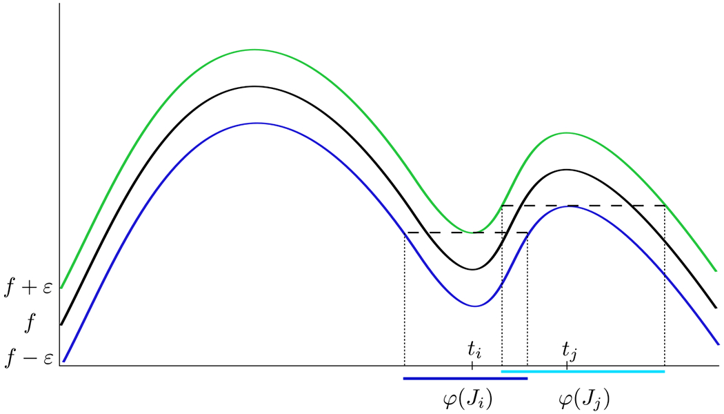
A graph of a function, f, as well as f ± ε. Here, t_i is a representative of a minimum with associated ε-minimum interval φ(J_i), and t_j is a representative of the ε-maximum interval φ(J_j). Notice that φ(J_i) ∩ φ(J_j) = ∅.

Definition 15. We define an order ◁ on ${\mathcal{J}}_{\epsilon }(f)$ as follows. Consider two relatively open intervals, $I,J\in {\mathcal{J}}_{\epsilon }(f)$, with y₁ < y₂ the endpoints of I and z₁ < z₂ the endpoints of J. Then I ◁ J if and only if either y_l < z_l or y₂ < z₂.

Theorem 1. The order ◁ on ${\mathcal{J}}_{\epsilon }(f)$ is a well-defined total order.

Proof. Consider two relatively open intervals $I,J\in {\mathcal{J}}_{\epsilon }(f)$, with y₁ < y₂ the endpoints of I and z₁ < z₂ the endpoints of J. Let u represent I and let v represent J. To prove that ◁ is well-defined, we must show that y₁ ≤ z₁ iff y₂ ≤ z₂.

The case where I ∩ J = ∅ is trivial, so we consider I ∩ J = ∅. It follows from Proposition 1 that when I ∩ J = ∅, then either $I\in {\mathcal{J}}_{\epsilon }^{\min }(f)$ and $J\in {\mathcal{J}}_{\epsilon }^{\max }(f)$ or vice versa. Now it follows from Proposition 4 that

$$u<v\Rightarrow y_1\le u\le z_1\text{and}{y}_2\le v\le z_2$$

and similarly

$$v<u\Rightarrow z_1\le v\le y_1\text{and}{z}_2\le u\le y_2.$$

This shows that the order is well defined. It now follows from Corollary 3 that the order is total. □

Theorem 2. ε-minimal intervals alternate with ε-maximal intervals.

Proof. Consider two adjacent ε-minimal intervals I₁ < I₂ with a₁ and a₂ the associated local minima. Assume without loss that a₁ > a₂. Then there exists t ∈ (a₁, a₂) such that t ∉ (f − ε)⁻¹(−∞, a₁ + ε), since otherwise I₁ and I₂ are not distinct. This implies that f(t) > a₁ + 2ε and therefore b := max_x∈[a1,a2] f(x) > a₁ + ε > a₂ + ε. Thus there is an ε-maximal interval J containing b. Since ◁ is a total order this implies I ◁ J ◁ K.

The argument ruling out two adjacent maxima is similar. □

4.1.6. Partial ordering between ${\mathcal{J}}_{\epsilon }(f_i)$

So far we have considered the representation of a single function f(t) in terms of a noise-level dependent collection of ε-minimal and ε-maximal intervals. However, many datasets include M functions f_i on the same domain [x₁, x₂]. There is a natural partial order on the union of the ε-extremal intervals.

Definition 16. Define the partially ordered set

$$\left(\underset{i}{\overset{M}{⨆}}{\mathcal{J}}_{\epsilon }\left(f_i\right),◁\right)$$

to be an extension of the total order of each ${\mathcal{J}}_{\epsilon }(f_i)$ as follows. If $I,J\in {\mathcal{J}}_{\epsilon }(f_i)$ for some i, define ◁ as in Definition 15. Now consider $I\in {\mathcal{J}}_{\epsilon }(f_i)$ and $J\in {\mathcal{J}}_{\epsilon }(f_j)$ for i ≠ j, with y₁ < y₂ the endpoints of I and z₁ < z₂ the endpoints of J. Then

$$I◁J\text{if and only if}{y}_2\le z_1.$$

We choose this order because overlapping ε-extremal intervals across functions indicate that the order of the respective local extrema is not decidable at the noise level of ε.

4.2. ε-extremal intervals for discrete time series

Time series have values measured at only a finite collection of times. In this section, we consider this case in more detail.

Definition 17. A set $\mathcal{D}≔{\{D_i\}}_{i=1}^M$ is a dataset on the interval [x₁, x₂] if $D_i≔{\{(z_k,h_k^i)\}}_{k=1}^N$ where

$$Z:=\{z_1=x_1,z_2,\mathrm{\dots },z_{N-1},z_N=x_2\},$$

is an ordered set with z_j < z_j+1 and the heights $h_k^i$ are measurements of the i^th variable at z_k. The components D_i will be referred to as time series.

The collection Z is independent of i. An example would be a collection of time series of gene expression, such as comes from RNAseq data. We note, however, that the independent variable is not required to be time.

Definition 18. Let f_i be the linear interpolation of D_i, and let ${\mathcal{J}}_{\epsilon }(f_i)$ be the ε-extremal intervals of the linear interpolation. Define ${\mathcal{K}}_{\epsilon }^{\min }(D_i)$ to be the set of relatively open intervals in [x₁, x₂] with endpoints in the set Z such that for each $I_i\in {\mathcal{J}}_{\epsilon }^{\min }(f_i)$, there exists $J_i\in {\mathcal{K}}_{\epsilon }^{\min }(D_i)$ satisfying

1. J_i ⊇ I_i, and

2. J_i is the minimal such interval; i.e. there does not exist an interval K_i with endpoints in Z such that J_i ⊉ K_i ⊇ I_i.

We define a function ${\beta }^{\min }:{\mathcal{K}}_{\epsilon }^{\min }(D_i)\to {\mathcal{J}}_{\epsilon }^{\min }(f_i)$ by β^min(J_i) = I_i that captures this relationship. Analogously, considering the linear interpolation – f_i, there is an analogous set of intervals ${\mathcal{K}}_{\epsilon }^{\max }(D_i)$ and a map β^max.

Since every local extremum of the linear interpolation f_i occurs at one of the points z_j ∈ Z, it is easy to see that the proof of Proposition 1 is still valid. Therefore we have

Proposition 5. For any $I,J\in {\mathcal{K}}_{\epsilon }^{\min }(D_i)$, I ∩ J = ∅.

Note that choosing f_i to be the linear interpolation of D_i is critical in order for this proposition to hold.

Definition 18 is a conservative definition in the sense that a minimum is guaranteed to occur within each interval I of ${\mathcal{K}}_{\epsilon }^{\min }(D_i)$ by restricting to ${\beta }^{\min }(I)\in {\mathcal{J}}_{\epsilon }^{\min }(f_i)$. In other words, Proposition 2 still holds for ${\mathcal{K}}_{\epsilon }^{\min }(D_i)$. However, minimality is lost in discretization and Proposition 3 does not hold for ${\mathcal{K}}_{\epsilon }^{\min }(D_i)$.

This widening of the ε-extremal intervals means that an ε-minimal interval and an ε-maximal interval can coincide. In other words, given $I\in {\mathcal{K}}_{\epsilon }^{\min }(D_i)$ and $J\in {\mathcal{K}}_{\epsilon }^{\max }(D_i)$, we can have that I = J, so that Proposition 3 does not hold. To address this issue, we remove these intervals from the sets ${\mathcal{K}}_{\epsilon }^{\min }(D_i)$ and ${\mathcal{K}}_{\epsilon }^{\max }(D_i)$.

Definition 19. Let ${\mathcal{K}}_{\epsilon }^{\cap }(D_i)$ be the intersection ${\mathcal{K}}_{\epsilon }^{\min }(D_i)\cap {\mathcal{K}}_{\epsilon }^{\max }(D_i)$. Then define

$$\begin{gathered} {\mathcal{I}}_{\epsilon }^{\min }(D_i):={\mathcal{K}}_{\epsilon }^{\min }(D_i)\backslash {\mathcal{K}}_{\epsilon }^{\cap }(D_i) \\ {\mathcal{I}}_{\epsilon }^{\max }(D_i):={\mathcal{K}}_{\epsilon }^{\max }(D_i)\backslash {\mathcal{K}}_{\epsilon }^{\cap }(D_i) \\ {\mathcal{I}}_{\epsilon }(D_i):={\mathcal{I}}_{\epsilon }^{\mathit{min}}(D_i)⨆{\mathcal{I}}_{\epsilon }^{\max }(D_i). \end{gathered}$$

We say that a time series D_i is ε-constant if and only if

$${\mathcal{I}}_{\epsilon }(D_i)=\varnothing .$$

In a slight abuse of nomenclature, we will refer to ${\mathcal{I}}_{\epsilon }(D_i)$ as the collection of ε-extremal intervals of D_i, and ${\mathcal{I}}_{\epsilon }^{\max }(D_i)$ and ${\mathcal{I}}_{\epsilon }^{\min }(D_i)$ will be called the ε-maximal and ε-minimal intervals of D_i, respectively. We say that

$${\mathcal{I}}_{\epsilon }\left(\mathcal{D}\right):=\underset{i}{\overset{M}{⨆}}{\mathcal{I}}_{\epsilon }\left(D_i\right)$$

is the set of ε-extremal intervals of the dataset.

Since ${\mathcal{I}}_{\epsilon }(\mathcal{D})\subseteq {\mathcal{K}}_{\epsilon }(\mathcal{D})$, all the results for ${\mathcal{K}}_{\epsilon }(\mathcal{D})$ hold on ${\mathcal{I}}_{\epsilon }(\mathcal{D})$.

The total order described in Definition 15, now applied to ${\mathcal{I}}_{\epsilon }({\mathcal{D}}_i)$, and the associated Theorem 1 proving the total order is well-defined, hold without changes – provided we again use the fact that all extrema of f_i occur at some z_j in the discretized time interval. Using that observation, we remark that the ε-minimal and ε-maximal intervals of ${\mathcal{I}}_{\epsilon }(D_i)$ still alternate, as in Theorem 2. We are now free to apply Definition 16 for the partial order ◁ on ${\mathcal{I}}_{\epsilon }(\mathcal{D})$, as restated here.

Definition 20. Define a partial order ◁ on the set ${\mathcal{I}}_{\epsilon }(\mathcal{D})$ as follows: Let $I\in {\mathcal{I}}_{\epsilon }(D_i)$ and $J\in {\mathcal{I}}_{\epsilon }(D_j)$ with y₁ < y₂ the endpoints of I and z₁ < z₂ the endpoints of J. If i = j, then I ◁ J if and only if either y₁ < z₁ or y₂ < z₂. If i ≠ j, then I ◁ J if and only if y₂ ≤ z₁.

4.3. Algorithms and software

4.3.1. Merge trees and branch decompositions

To calculate merge trees and branch decompositions for a discrete time series $D_i=\{z_j,h_j^i\}$, we follow Smirnov and Morozov [34], who provide pseudocode for Kruskals algorithm and a helper function called FindDeepest. This combination of algorithms has O(m log n) complexity for a merge tree with n nodes and m edges. We briefly summarize these algorithms here.

Let Z be the ordered set of time points {z₁, …, z_N} and let f_i be the linear interpolation as before, with $f_i(z_j)=h_j^i$. We form a linear graph G, where the vertices of G are labeled by the elements of Z, and edges in G connect and z_j and z_j+1 for all i. For brevity, we will drop subscripts where the context allows, and we will refer to a vertex in G as an element z ∈ Z.

Definition 21 ([34]). For $h\in \mathbb{R}$, the sublevel graph at h, denoted G_h, is the subgraph induced by the vertices Z′ ⊆ Z whose function values f_i(z) for z ∈ Z′ do not exceed h. The representative of vertex z at level h ≥ f_i(z) is the vertex y ∈ Z with the minimum function value in the connected component of G_h containing z.

Definition 22 ([34]). The merge tree of f_i on G is the tree on the vertex set of G that has an edge (z, y), with f_i(z) < f_i(y), if the connected component of z in G_fi(z)(z) is a subset of the connected component of y in G_fi(y), and there is no vertex x with f_i(z) < f_i(x) < f_i(y) such that the connected component of z is a subset of the connected component of x in G_fi(x).

The algorithm of Smirnov and Morozov [34] is based on a representation of each vertex z in the merge tree by a triplet of vertices (z, s, y), where vertex z represents itself at levels h ∈ [f_i(z), f_i(s)), and y becomes its representative at level f_i(s). We make the following observations:

• if z is a vertex representing the global minimum of f_i, then the triplet attached to z will be (z, z, z);

• if z is any other local minimum of f_i and hence a leaf of the merge tree, then the triplet associated to z is (z, s, y) with z ≠ s ≠ y and f_i(y) < f_i(z) < f_i(s);

• if z is any other non-leaf vertex of G, then its triplet representation is (z, z, y) with f_i(y) < f_i(z).

Note that for any leaf z of the merge tree with triplet (z, s, y), the interval [f_i(z), f_i(s)) represents a branch in the branch decomposition. For z with a triplet (z, z, z), the branch is [f_i(z), b₀], where b₀ is the global maximum of f_i. The normalized branch decomposition is then the collection {[0, f_i(s) − f_i(z))}∪{[0, b₀ − f_i(z)]} for every triplet in the branch decomposition. Therefore the algorithms of [34] calculate both the merge tree and the normalized branch decomposition simultaneously.

We implemented Algorithms 1 and 2 of [34] in Python 3 [21], along with a post-processing function to isolate the leaves of the merge tree using the fact that non-leaf vertices always have the triplet form (z, z, y) with f_i(y) < f_i(z). When there are two minima of identical depth, the one that occurs first in time is chosen to represent the triplet as in Definition 9.

4.3.2. ε-extremal intervals

Once the leaves are isolated, we calculate, for some specified noise level ε, the ε-minimal interval associated to each minimum. First, we remove all normalized branches that are not greater than 2ε. Then we take each representative z in the remaining triplets (z, s, y), and grow a ball around z until the associated function values f_i(z−δ₁) and f_i(z+δ₂) meet or exceed a distance of 2ε from f_i(z). This constraint arises because we are constructing the connected component of the sublevel set (f_i − ε)⁻¹(−∞, f_i(z) + ε) that contains z. So we are seeking the largest set of vertices Z′ ⊆ Z such that the subgraph of G induced by Z′ is connected, and any v ∈ Z′ satisfies f_i(v) − ε ∈ (−∞, f_i(z) + ε), or equivalently, f_i(v) − ε < f_i(z) + ε.

In order to find the dual merge tree, dual branch decomposition, and associated ε-maximal intervals, we simply reflect the curve f_i over the z-axis to get −f_i, and repeat exactly the same procedure. The calculation of ε-extremal intervals given the triplets is at worst linear in the number of time points in the time series.

Once we have all of the ε-extremal intervals for a dataset, ${\mathcal{I}}_{\epsilon }(\mathcal{D})$, we impose the partial order in Definition 20. All of this functionality is in the open source software [21], along with Jupyter notebooks that generate the figures for the applications in Section 3.

4.3.3. Graph distance

In Application 2, we use a graph distance to calculate similarity between the transitive closures of Hasse diagrams. This graph distance gives roughly the proportion of dissimilar edges between $H_{\epsilon }^C({\mathcal{D}}_1)$ and $H_{\epsilon }^C({\mathcal{D}}_2)$.

Definition 23. For two node-labeled graphs G(V, E, ℓ) and G′(V′, E′, ℓ′), a bijection ϕ : V → V′ is a graph isomorphism if and only if

• (v₁, v₂) ∈ E ⇔ (ϕ(v₁), ϕ(v₂)) ∈ E′ for all v₁, v₂ ∈ V,

• ℓ(v) = ℓ′(ϕ(v)) for all v ∈ V.

Definition 24. For two node-labeled graphs G(V, E, ℓ) and G′(V′, E′, ℓ′) the directed maximum common edge induced subgraph (DMECS) problem is to find some ordered pair (W, W′) with W ⊆ E and W′ ⊆ E′ such that if

$$\begin{gathered} U=\left\{v_1\in V|\left(v_1,v_2\right)\in Wor\left(v_2,v_1\right)\in W\right\} \\ U\prime =\left\{v_1\in V\prime |\left(v_1,v_2\right)\in W\prime or\left(v_2,v_1\right)\in W\prime \right\} \end{gathered}$$

then the graphs H = (U, W, ℓ|_U) and H′ = (U′, W′, ℓ′|_U′) are isomorphic and the value of |W| = |W′| is maximized. Here H and H′ are edge-induced subgraphs of G and G′. |W| is maximized if for all Z ⊆ E and Z′ ⊆ E′ such that Z and Z′ induce isomorphic subgraphs of G and G′,

$$\left|Z\right|\le \left|W\right|.$$

We define DMCES(G, G′) = |W| where |W| is maximized.

It is shown in [36] that

$$d\left(G,G\prime \right)=1-\frac{\mathrm{DMCES}\left(G,G\prime \right)}{\max \left(\left|E\right|,\left|E\prime \right|\right)}.$$

is a metric on the space of node-labeled, directed graphs. Since by definition

$$DMCES\left(G,G\prime \right)\le \max \left(\left|E\right|,\left|E\prime \right|\right),$$

distance varies between 0 (most similar) and 1 (least similar).

As shown in [36], there is a polynomial-time reduction of the DMCES problem to the maximum clique problem and polynomial-time reduction of the graph isomorphism problem to the DMCES problem. Thus DMCES is no easier than the graph isomorphism problem and no harder than the maximum clique problem. This suggests that computing the DMCES problem is exponentially hard but no harder than NP-complete problems. We use an algorithm from [36] to compute the DMCES problem which leverages the special structure of the Hasse diagrams produced from datasets; namely that the partial order is built from the collection of total orders that arise from each individual time series.

5. Discussion

The method described in this paper assigns to a time series a collection of partially ordered intervals that are dependent upon a level of measurement uncertainty ε. Each interval is guaranteed to contain either a maximum or a minimum of every continuous function that is ε-close to the time series. We are particularly focused on applications in molecular and cellular biology where ’omics data can measure expression levels of thousands of genes; however, this approach is widely applicable.

Due to experimental challenges, a typical time series has 10-20 time points with time resolution of minutes to hours, and significant levels of measurement error. We do not assume that the measured variables are statistically independent; in fact this dependence carries information about the interactions between the components of the system which are of great interest. There are methods that use time series to deduce a structure of the underlying causal network [2, 3, 4, 5], i.e. which genes up-regulate or down-regulate other genes. These methods rely on sequencing of time points when genes achieve their peak expression, lowest expression, or time points when they pass the half saturation point. Since this is the time where maximal rate of change occurs, we may alternatively approximate the derivative of the time series and turn the problem of finding the sequence of times with maximal rates of change to the problem of finding extrema.

Our work is closely related to work on merge trees and persistence homology [18, 37, 38]. Persistence type methods use topological data analysis to extract the most prominent extrema. Since the most persistent features have large amplitude, and we are interested in all levels where extrema appear and disappear, the 0-persistence of f gives closely related, but complementary results to ours.

Similar ideas to those presented in this paper have been used in [39] in the context of 2D uncertain scalar fields. Their goal is to describe mandatory critical points for 2D data for which upper and lower bounding scalar fields f⁻ and f⁺ are given. The mandatory critical points are characterized by regions of the plane called critical components where the critical point is guaranteed to occur for any realization of a scalar field within f⁻ and f⁺, and by critical intervals in $\mathbb{R}$ which bound the admissible height of the critical point. These critical components correspond in our approach to ε-minimal intervals when f⁺ = f + ε and f⁻ = f − ε.

Our approach can be viewed as an adaptation of the technique in [39] to time series data, with some important differences. Since the time series data are assumed to arise from a continuous process, we first analyze continuous functions and only then extend it to the discrete time series data. Moreover, we do not assume that the upper (f⁺) and lower (f⁻) bounds are given; rather we parameterize these in terms of parameter ε and analyze a range of values of ε. This aspect is very important in the applications we present in Section 3. In these applications, we analyze multiple time series, construct partial orders of ε-extremal intervals, and use the partial orders to compare models to time series as well as quantify differences between time series replicates.

The two applications of our technique use microarry data. In the first application, the presented analysis allows the rejection of DSGRN network models [1, 12] that cannot reproduce the experimentally observed sequences of minima and maxima of microarray time series. For a proposed network model, DSGRN computes all possible sequences of minima and maxima that can be produced by the network, across all parameters. This data can be then compared to a partial order computed from the experimental time series data, at different levels of assumed experimental measurement uncertainty ε. We illustrate our approach on data from the yeast cell cycle, where the regulatory network is well-described and has substantial experimental validation [22, 40, 28, 41, 31, 42]. We show that the network model can reproduce experimental data at a low level of assumed experimental noise, but cannot reproduce data where we artificially swap labels on the time series. Swapping labels is equivalent to making the model incorrect, and such a model is consistent with data only at very high levels of noise (28% of the total signal amplitude).

In our second application, we study again the gene regulatory network that controls the cell-cycle-transcriptional program [32, 33, 28, 31]. The network of serially-activated transcription factors activates other transcription factors at appropriate phase of the cell cycle and thus plays a key role in establishing a cell cycle generating order in cellular transcription. There is an ongoing debate in the field on the role of this network in controlling cell-cycle-regulated transcription and in the ordering of cell-cycle events [43, 44]. A reproducible ordering of gene expression, which we observe in this paper, argues for precise control of the transcriptional program and provides further supporting evidence for the importance of a cell-cycle gene regulatory network.

The problem of aligning data from different experiments and evaluating the similarity of two experiments is a problem in biology that goes beyond the study of cell cycles. Circadian clock networks also control large, well-ordered programs of phase-specific gene expression [45, 46], and perturbations to those programs are likely to be found in clock-associated diseases. Ordering the expression of genes is also a fundamental mechanism for the assembly of a variety of protein complexes [47]. Thus, the ability to accurately compare ordering in gene expression will be useful for identifying perturbations in complex formation, circadian regulation, as well as cell-cycle control. The approach presented in this paper is applicable to any experimental time series data where comparison and evaluation of similarity of ordering is desired.

A. Yeast data analysis

Time-series transcriptomic data for one replicate of wild-type yeast Saccharomyes cerevisiae were previously published in [28]. Microarray (Affymetrix Yeast Genome 2.0) expression data were normalized as previously described [28], although for this study Affymetrix probe IDs were re-annotated using Affymetrix Yeast Genome 2.0 microarray annotation 35. Expression data were aligned to a common cell-cycle time line using the CLOCCS (Characterizing Loss of Cell Cycle Synchrony) [29] population synchrony model, as previously described [28]. Briefly, the CLOCCS model allows multiple time-series experiments to be aligned to a common cell-cycle timeline, using experimentally-derived yeast budding data. The CLOCCS model converts time points in the series to life points, which indicate the progression through the cell cycle. Expression data for both replicates were interpolated to integer life points with an interval of one using a Piecewise Cubic Hermite Interpolating Polynomial (PCHIP) spline. Life points were then trimmed so both replicate time series were of identical location and duration in the cell cycle.

References

- [1].Cummins B, Gedeon T, Harker S, Mischaikow K, Model rejection and parameter reduction via time series, SIAM J. Appl. Dyn. Syst to appear. [DOI] [PMC free article] [PubMed] [Google Scholar]
- [2].Albert R, Network inference, analysis, and modeling in systems biology, The Plant cell 19 (11) (2007) 3327–3338. [DOI] [PMC free article] [PubMed] [Google Scholar]
- [3].Sugihara G, May R, Ye H, Hsieh C, Deyle E, Fogarty M, Munch S, Detecting Causality in Complex Ecosystems, Science 338 (2016) 496. [DOI] [PubMed] [Google Scholar]
- [4].Cummins B, Gedeon T, Spendlove K, On the efficacy of state space reconstruction methods in determining causality, SIAM J. Appl. Dyn. Syst 14 (1) (2015) 335–381. [Google Scholar]
- [5].McGoff K, Guo X, Deckard A, Kelliher C, Leman A, Francey L, Hogenesch J, Haase S, Harer J, The Local Edge Machine: inference of dynamic models of gene regulation, Genome Biology 17 (1) (2016) 214. [DOI] [PMC free article] [PubMed] [Google Scholar]
- [6].Akutsu T, Miyano S, Kuhara S, Inferring qualitative relations in genetic networks and metabolic pathways, Bioinformatics 16 (8) (2000) 727–734. doi: 10.1093/bioinformatics/16.8.727 URL https://academic.oup.eom/bioinformatics/article/16/8/727/190308 [DOI] [PubMed] [Google Scholar]
- [7].Brunton SL, Proctor JL, Kutz JN, Discovering governing equations from data by sparse identification of nonlinear dynamical systems, Proceedings of the National Academy of Sciences 113 (15) (2016) 3932–3937. doi: 10.1073/pnas.1517384113 URL http://www.pnas.org/content/113/15/3932 [DOI] [PMC free article] [PubMed] [Google Scholar]
- [8].Maucher M, Kracher B, Khl M, Kestler HA, Inferring Boolean network structure via correlation, Bioinformatics 27 (11) (2011) 1529–1536. doi: 10.1093/bioinformatics/btr166 URL https://academic.oup.com/bioinformatics/article/27/11/1529/216683 [DOI] [PubMed] [Google Scholar]
- [9].Lähdesmäki H, Shmulevich I, Yli-Harja O, On learning gene regulatory networks under the boolean network model, Machine Learning 52 (1) (2003) 147–167. doi: 10.1023/A:1023905711304 URL 10.1023/A:1023905711304 [DOI] [Google Scholar]
- [10].Barker NA, Myers CJ, Kuwahara H, Learning genetic regulatory network connectivity from time series data, IEEE/ACM Transactions on Computational Biology and Bioinformatics 8 (1) (2011) 152–165. doi: 10.1109/TCBB.2009.48. [DOI] [PubMed] [Google Scholar]
- [11].Carré C, Mas A, Krouk G, Reverse engineering highlights potential principles of large gene regulatory network design and learning, NPJ Systems Biology and Applications 3 (17). doi: 10.1038/s41540-017-0019-y. [DOI] [PMC free article] [PubMed] [Google Scholar]
- [12].Cummins B, Gedeon T, Harker S, Mischaikow K, Mok K, Combinatorial Representation of Parameter Space for Switching Systems, SIAM J. Appl. Dyn. Syst 15 (4) (2016) 2176–2212. [DOI] [PMC free article] [PubMed] [Google Scholar]
- [13].Albert R, Collins JJ, Glass L, Introduction to Focus Issue: Quantitative approaches to genetic networks, Chaos 23 (2) (2013) 025001. [DOI] [PubMed] [Google Scholar]
- [14].Edwards R, Chaos in neural and gene networks with hard switching, Diff. Eq. Dyn. Sys (9) (2001) 187–220. [Google Scholar]
- [15].Glass L, Kauffman SA, The logical analysis of continuous, non-linear biochemical control networks., Journal of Theoretical Biology 39 (1) (1973) 103–29. URL http://www.ncbi.nlm.nih.gov/pubmed/4741704 [DOI] [PubMed] [Google Scholar]
- [16].Thomas R, Regulatory networks seen as asynchronous automata: A logical description, Journal of Theoretical Biology 153 (1991) 1–23. doi: 10.1016/S0022-5193(05)80350-9. [DOI] [Google Scholar]
- [17].Harker S, Dsgrn software doi: 10.5281/zenodo.1210003 URL https://github.com/shaunharker/DSGRN [DOI]
- [18].Edelsbrunner H, Harer JL, Computational topology, American Mathematical Society, Providence, RI, 2010. [Google Scholar]
- [19].Morozov D, Beketayev K, Weber G, Interleaving distance between merge trees, Discrete and Computational Geometry 49 (2013) 22–45. [Google Scholar]
- [20].Morozov D, Weber G, Distributed merge trees, in: Proceedings of the Annual Symposium on Principles and Practice of Parallel Programming, 2013, pp. 93–102. [Google Scholar]
- [21].Cummins B, Nerem R, ε-minimal interval software v0.4 doi: 10.5281/zenodo.3405579. URL https://github.com/breecummins/min_interval_posets [DOI] [Google Scholar]
- [22].Cho CY, Kelliher CM, Haase SB, The cell-cycle transcriptional network generates and transmits a pulse of transcription once each cell cycle, Cell Cycle (2019) 1–16 doi: 10.1080/15384101.2019.1570655 URL https://www.ncbi.nlm.nih.gov/pubmed/30668223 [DOI] [PMC free article] [PubMed] [Google Scholar]
- [23].Davey BA, Priestley HA, Introduction to lattices and order, Cambridge university press, 2002. [Google Scholar]
- [24].Bunke H, Riesen K, Recent advances in graph-based pattern recognition with applications in document analysis, Pattern Recognition 44 (5) (2011) 1057–1067. doi: 10.1016/j.patcog.2010.11.015. URL http://www.sciencedirect.com/science/article/pii/S003132031000542X [DOI] [Google Scholar]
- [25].Conte D, Foggia P, Sansone C, Vento M, Thirty years of graph matching in pattern recognition, International journal of pattern recognition and artificial intelligence 18 (03) (2004) 265–298. URL http://www.worldscientific.com/doi/abs/10.1142/S0218001404003228 [Google Scholar]
- [26].Livi L, Rizzi A, Parallel algorithms for tensor product-based inexact graph matching, in: The 2012 International Joint Conference on Neural Networks (IJCNN), 2012, pp. 1–8. doi: 10.1109/IJCNN.2012.6252681. [DOI] [Google Scholar]
- [27].Fu JJ, Approximate pattern matching in directed graphs, in: Hirschberg G. Myers(Eds.), Combinatorial Pattern Matching, no. 1075 in Lecture Notes in Computer Science, Springer; Berlin Heidelberg, 1996, pp. 373–383. doi: 10.1007/3-540-61258-0_27 URL http://link.springer.com/chapter/10.1007/3-540-61258-0_27 [DOI] [Google Scholar]
- [28].Orlando DA, Lin CY, Bernard A, Wang JY, Socolar JE, Iversen S, Hartemink AJ, Haase SB, Global control of cell-cycle transcription by coupled cdk and network oscillators, Nature 453 (7197) (2008) 944–7. URL http://www.ncbi.nlm.nih.gov/entrez/query.fcgi?cmd=Retrieve&db=PubMed&dopt=Citation&list_uids=18463633 [DOI] [PMC free article] [PubMed] [Google Scholar]
- [29].Orlando DA, Lin CY, Bernard A, Iversen ES, Hartemink AJ, Haase SB, A probabilistic model for cell cycle distributions in synchrony experiments, Cell Cycle 6 (2007) 478–488. [DOI] [PubMed] [Google Scholar]
- [30].Kelliher CM, Leman AR, Sierra CS, Haase SB, Investigating conservation of the cell-cycle-regulated transcriptional program in the fungal pathogen, cryptococcus neoformans, PLoS genetics 12 (12) (2016) e1006453. [DOI] [PMC free article] [PubMed] [Google Scholar]
- [31].Simmons Kovacs LA, Mayhew MB, Orlando DA, Jin Y, Li Q, Huang C, Reed SI, Mukherjee S, Haase SB, Cyclin-dependent kinases are regulators and effectors of oscillations driven by a transcription factor network, Mol Cell 45 (5) (2012) 669–79. doi:S1097-2765(12)00043-3[pii]10.1016/j.molcel.2011.12.033 URL http://www.ncbi.nlm.nih.gov/entrez/query.fcgi?cmd=Retrieve&db=PubMed&dopt=Citation&list_uids=22306294 [DOI] [PMC free article] [PubMed] [Google Scholar]
- [32].Bristow SL, Leman AR, Simmons Kovacs LA, Deckard A, Harer J, Haase SB, Checkpoints couple transcription network oscillator dynamics to cell-cycle progression, Genome Biol 15 (9) (2014) 446. doi: 10.1186/s13059-014-0446-7. URL http://www.ncbi.nlm.nih.gov/pubmed/25200947 [DOI] [PMC free article] [PubMed] [Google Scholar]
- [33].Cho CY, Motta FC, Kelliher CM, Deckard A, Haase SB, Reconciling conflicting models for global control of cell-cycle transcription, Cell Cycle (2017) 1–14 doi: 10.1080/15384101.2017.1367073 URL https://www.ncbi.nlm.nih.gov/pubmed/28934013 [DOI] [PMC free article] [PubMed] [Google Scholar]
- [34].Smirnov D, Morozov D, Triplet merge trees, in: Topological Methods in Data Analysis and Visualization V (Proceedings of TopoInVis 2017), To appear. [Google Scholar]
- [35].Pascucci V, Cole-Mclaughlin K, Scorzelli G, Multi-resolution computation and presentation of contour trees, in: IASTED conference on Visualization, Imaging, and Image Processing, 2004. [Google Scholar]
- [36].Nerem R, Crawford-Kahrl P, Cummins B, Gedeon T, A poset metric from the directed maximum common edge subgraph (2019). arXiv:arXiv:1910.14638. [Google Scholar]
- [37].Carlsson G, Topology and data, Bull. Amer. Math. Soc. (NS) 46 (2) (2009) 255–308. [Google Scholar]
- [38].Zomorodian A, Carlsson G, Computing persistent homology, Discrete & Computational Geometry 33 (2) (2005) 249–274. [Google Scholar]
- [39].Günther D, Salmon J, Tierny J, Mandatory critical points of 2d uncertain scalar fields, in: Computer Graphics Forum, Vol. 33, Wiley Online Library, 2014, pp. 31–40. [Google Scholar]
- [40].Haase SB, Wittenberg C, Topology and control of the cell-cycle-regulated transcriptional circuitry, Genetics 196 (1) (2014) 65–90. doi: 10.1534/genetics.113.152595. URL http://www.ncbi.nlm.nih.gov/pubmed/24395825 [DOI] [PMC free article] [PubMed] [Google Scholar]
- [41].Pramila T, Wu W, Miles S, Noble WS, Breeden LL, The forkhead transcription factor hcm1 regulates chromosome segregation genes and fills the s-phase gap in the transcriptional circuitry of the cell cycle, Genes Dev 20 (16) (2006) 2266–78. URL http://www.ncbi.nlm.nih.gov/entrez/query.fcgi?cmd=Retrieve&db=PubMed&dopt=Citation&list_uids=16912276 [DOI] [PMC free article] [PubMed] [Google Scholar]
- [42].Simon I, Barnett J, Hannett N, Harbison CT, Rinaldi NJ, Volkert TL, Wyrick JJ, Zeitlinger J, Gifford DK, Jaakkola TS, Young RA, Serial regulation of transcriptional regulators in the yeast cell cycle, Cell 106 (6) (2001) 697–708. URL http://www.ncbi.nlm.nih.gov/entrez/query.fcgi?cmd=Retrieve&db=PubMed&dopt=Citation&list_uids=11572776 [DOI] [PubMed] [Google Scholar]
- [43].Rahi SJ, Pecani K, Ondracka A, Oikonomou C, Cross FR, The cdk-apc/c oscillator predominantly entrains periodic cell-cycle transcription, Cell 165 (2) (2016) 475–87. doi: 10.1016/j.cell.2016.02.060 URL https://www.ncbi.nlm.nih.gov/pubmed/27058667 [DOI] [PMC free article] [PubMed] [Google Scholar]
- [44].Shedden K, Cooper S, Analysis of cell-cycle gene expression in saccharomyces cerevisiae using microarrays and multiple synchronization methods, Nucleic Acids Research 30 (13) (2002) 2920–9. [DOI] [PMC free article] [PubMed] [Google Scholar]
- [45].Mure LS, Le HD, Benegiamo G, Chang MW, Rios L, Jillani N, Ngotho M, Kariuki T, Dkhissi-Benyahya O, Cooper HM, Panda S, Diurnal transcriptome atlas of a primate across major neural and peripheral tissues, Science doi: 10.1126/science.aao0318 URL http://science.sciencemag.org/content/sci/early/2018/02/07/science.aao0318.full.pdf [DOI] [PMC free article] [PubMed] [Google Scholar]
- [46].Zhang R, Lahens NF, Ballance HI, Hughes ME, Hogenesch JB, A circadian gene expression atlas in mammals: implications for biology and medicine, Proc Natl Acad Sci USA 111 (45) (2014) 16219–24. doi: 10.1073/pnas.1408886111 URL http://www.ncbi.nlm.nih.gov/pubmed/25349387 [DOI] [PMC free article] [PubMed] [Google Scholar]
- [47].Simmons Kovacs LA, Orlando DA, Haase SB, Transcription networks and cyclin/cdks: the yin and yang of cell cycle oscillators, Cell Cycle 7 (17) (2008) 2626–9. doi:6515[pii] URL http://www.ncbi.nlm.nih.gov/entrez/query.fcgi?cmd=Retrieve&db=PubMed&dopt=Citation&list_uids=18758238 [DOI] [PubMed] [Google Scholar]