New 3D graphical representation of DNA sequence based on dual nucleotides

Abstract

We introduce a 3D graphical representation of DNA sequences based on the pairs of dual nucleotides (DNs). Based on this representation, we consider some mathematical invariants and construct two 16-component vectors associated with these invariants. The vectors are used to characterize and compare the complete coding sequence part of beta globin gene of nine different species. The examination of similarities/dissimilarities illustrates the utility of the approach.

1. Introduction

The number of biological sequences is rapidly increasing in the biological database. It is one of the challenges for bio-scientists to analyze mathematically the large volume of biological sequence data. It is good to use the graphic representation to study complicated biological systems because it can provide an intuitive picture and help people gain useful insights. Similar graphical approaches have also been used to deal with a wide variety of biological problems. For instance, various graphic approaches have been successfully used to study enzyme-catalyzed system (see, e.g., King and Altman, 1956, Chou et al., 1979, Chou and Forsen, 1980, Chou and Liu, 1981, Zhou and Deng, 1984, Chou, 1989, Chou, 1990; Kuzmic et al., 1992, Lin and Neet, 1990), protein folding kinetics (Chou, 1990, Chou, 1993), condon usage (Chou and Zhang, 1992, Zhang and Chou, 1994), HIV reverse transcriptase inhibition mechanisms (Althaus et al., 1993a, Althaus et al., 1993b, Althaus et al., 1993c) and base frequency distribution in the anti-sense strands (Chou and Zhang, 1996). Recently, the images of cellular automata were also used to represent biological sequences (Xiao et al., 2005a), predict protein subcellular location (Xiao et al., 2006a), investigate HBV virus gene missense mutation (Xiao et al., 2005b) and HBV viral infections (Xiao et al., 2006b), as well as analyze the fingerprint of SARS coronavirus (Wang et al., 2005).

As for an important part of graphical techniques, graphical representations of DNA sequences have been proposed by several authors (Zhang, 1991, Nandy, 1994, Nandy and Nandy, 2003, Liao and Wang, 2004, Randic et al., 2003, Liu et al., 2006; Zhang and Chen, 2006). Some of them, for example Nandy’ graphical representation (Nandy, 1994), are accompanied by some loss of visual information associated with crossing and overlapping of the curve with itself. In order to avoid the limitations related to crossing and overlapping, Liao (Liao and Wang, 2004) and Randic (Randic and Vracko, 2000, Randic et al., 2003) present their 2D or 3D graphical representations. However, their approaches are associated with the computations of D/D, L/L and leading eigenvalue, which need a great deal of running time and memory space.

Moreover, the dinucleotide analysis has also been tried by several previous authors. Randic (2000) proposed a condensed representation of DNA based on pairs of nucleotides. This approach can offer fast, qualitative comparisons of DNA and allow quantitative comparisons of DNA from different sources. Wu et al. (2003) and Liu et al. (2006) proposed their analysis approaches based on neighboring nucleotides of DNA sequence, which reveal the biology information hidden between the dual nucleotides (DNs). Qi and Qi (2007) also suggest a dinucleotide analysis method to reveal the biology information of DNA sequences.

Recently, Qi and Fan (2007) proposed a 3D graphical representation of DNA sequence based on a pair of nucleotides. Based on similar research object (3D graphical representation of DNA sequence based on a pair of nucleotides), in this paper we introduce a new 3D graphical representation (3D-DN curve) of DNA primary sequences, in which there is also no loss of information in the transfer of data from a DNA sequence to its mathematical representation. Our representation is different from that of PN-curve (Qi and Fan, 2007). The two papers are highly dissimilar with respect to each other in many aspects: the methods and contents of research, the map used to construct graphical representation, the graphical curve and numerical invariants characterizing DNA sequences. The introduced representation is simple and direct, and gives us more biology information based on DNs.

2. 3D graphical representation of DNA sequences based on dual nucleotides

Given a DNA primary sequence, there are 16 kinds of the pairs of the neighboring nucleotides. These pairs can be classified as four categories based on their chemical properties: purine-DN {AG, GA}/pyrimidine-DN {CT, TC}, amino-DN {AC, CA}/keto-DN {GT, TG}, weak-H bond DN {AT, TA}/strong-H bond DN {CG, GC} and repeat-DN {AA, CC, GG, TT}. Then we design a $4\times 4$ matrix and give a new 3D graphical representation of DNA sequences. We arrange 16 DNs in a $4\times 4$ matrix according to the above four categories. The matrix is

$$\left[\begin{array}{cccc}\hfill \mathrm{AG}\hfill & \hfill \mathrm{GA}\hfill & \hfill \mathrm{CT}\hfill & \hfill \mathrm{TC}\hfill \\ \hfill \mathrm{AC}\hfill & \hfill \mathrm{CA}\hfill & \hfill \mathrm{GT}\hfill & \hfill \mathrm{TG}\hfill \\ \hfill \mathrm{AT}\hfill & \hfill \mathrm{TA}\hfill & \hfill \mathrm{CG}\hfill & \hfill \mathrm{GC}\hfill \\ \hfill \mathrm{AA}\hfill & \hfill \mathrm{CC}\hfill & \hfill \mathrm{GG}\hfill & \hfill \mathrm{TT}\hfill \end{array}\right]\text{.}$$

Every element of the matrix has a corresponding index $(i,j)$, $i=0,1,2,3$; $j=0,1,2,3$. Based on the index, we assign one DN as follows:

$$(0,0,0)\to \mathrm{AG},(0,1,0)\to \mathrm{GA},(0,2,0)\to \mathrm{CT},(0,3,0)\to \mathrm{TC}\text{,}(1,0,0)\to \mathrm{AC},(1,1,0)\to \mathrm{CA},(1,2,0)\to \mathrm{GT},(1,3,0)\to \mathrm{TG}\text{,}(2,0,0)\to \mathrm{AT},(2,1,0)\to \mathrm{TA},(2,2,0)\to \mathrm{CG},(2,3,0)\to \mathrm{GC}\text{,}(3,0,0)\to \mathrm{AA},(3,1,0)\to \mathrm{CC},(3,2,0)\to \mathrm{GG},(3,3,0)\to \mathrm{TT}\text{.}$$

That is to say, we assign every DN to its corresponding index $(x,y)$, respectively, while the corresponding curve extending along with z-axes. In detail, let $G=g_1{g}_2\dots$ be an arbitrary DNA primary sequence. Then we define a map $\phi$ as follows:

$$\phi (g_i{g}_{i+1})=\left\{\begin{array}{cc}(0,0,i)\hfill & \mathrm{if}{g}_i{g}_{i+1}=\mathrm{AG},\hfill \\ (0,1,i)\hfill & \mathrm{if}{g}_i{g}_{i+1}=\mathrm{GA},\hfill \\ (0,2,i)\hfill & \mathrm{if}{g}_i{g}_{i+1}=\mathrm{CT},\hfill \\ (0,3,i)\hfill & \mathrm{if}{g}_i{g}_{i+1}=\mathrm{TC},\hfill \\ (1,0,i)\hfill & \mathrm{if}{g}_i{g}_{i+1}=\mathrm{AC},\hfill \\ (1,1,i)\hfill & \mathrm{if}{g}_i{g}_{i+1}=\mathrm{CA},\hfill \\ (1,2,i)\hfill & \mathrm{if}{g}_i{g}_{i+1}=\mathrm{GT},\hfill \\ (1,3,i)\hfill & \mathrm{if}{g}_i{g}_{i+1}=\mathrm{TG},\hfill \\ (2,0,i)\hfill & \mathrm{if}{g}_i{g}_{i+1}=\mathrm{AT},\hfill \\ (2,1,i)\hfill & \mathrm{if}{g}_i{g}_{i+1}=\mathrm{TA},\hfill \\ (2,2,i)\hfill & \mathrm{if}{g}_i{g}_{i+1}=\mathrm{CG},\hfill \\ (2,3,i)\hfill & \mathrm{if}{g}_i{g}_{i+1}=\mathrm{GC},\hfill \\ (3,0,i)\hfill & \mathrm{if}{g}_i{g}_{i+1}=\mathrm{AA},\hfill \\ (3,1,i)\hfill & \mathrm{if}{g}_i{g}_{i+1}=\mathrm{CC},\hfill \\ (3,2,i)\hfill & \mathrm{if}{g}_i{g}_{i+1}=\mathrm{GG},\hfill \\ (3,3,i)\hfill & \mathrm{if}{g}_i{g}_{i+1}=\mathrm{TT}.\hfill \end{array}\right)$$

The map $\phi$ maps G into a plot set. For example, the corresponding plot set of the sequence ATGGTGCACC is {(2, 0, 1), (1, 3, 2), (3, 2, 3), (1, 2, 4), (1, 3, 5), (2, 3, 6), (1, 1, 7), (1, 0, 8), (3, 1, 9)}. The corresponding plot set is called as characteristic plot set. The curve connected all plots of the characteristic plot set in turn is called 3D-DN curve. In Table 1 and Fig. 1 , we show the corresponding coordinates and the 3D graphical representation of the sequence, respectively.

Table 1.

Cartesian 3D coordinates for the sequence ATGGTGCACC of the coding sequence of the first exon of human $\beta$-globin gene

Base	DNs	x	y	z
1	AT	2	0	1
2	TG	1	3	2
3	GG	3	2	3
4	GT	1	2	4
5	TG	1	3	5
6	GC	2	3	6
7	CA	1	1	7
8	AC	1	0	8
9	CC	3	1	9

Fig. 1.

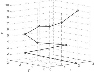
Characteristic curve of the sequence ATGGTGCACC, the dots denote the DNs making up the sequence.

From the construction of the $4\times 4$ matrix, we know that their designs are not unique. There are 16 kinds of DNs, so they have $16!$ combinations. But we design the $4\times 4$ matrix based on the classifications of nucleotides. In this paper, we only consider the above $4\times 4$ matrix to illustrate our scheme.

3. Numerical characterization of DNA sequences

Given a DNA sequence with the length of N. Based on the definition of the map $\phi$, we can have a set of points $(x_i,y_i,z_i)$, $i=1,2,\dots ,N-1$, and the correspondence between the DNs and the points is one-to-one. In order to find some of the invariants sensitive to the form of the characteristic curve we will transform the 3D graphical representation of the characteristic curve into another mathematical object. Firstly, let $K^{\mathit{ab}}$ denote the total number of the DN ab appearing in the given sequence, $a\in \{A,C,G,T\}$, $b\in \{A,C,G,T\}$. The vertex (dot) $V_1$ denotes the first dot $(x_1,y_1,z_1)$ of the 3D-DN curve. The vertex (dot) $V_i$ denotes the ith dot $(x_i,y_i,z_i)$ of the 3D-DN curve. Then let $d^{\mathit{ab}}$ denote the sum of geometrical lengths of edges between vertices (dots) $V_1$ and $V_{\mathit{ab}}$ of the 3D-DN curve, where $V_{\mathit{ab}}$ denotes the vertex representing the DN ab appearing in the given sequence. The parameter $p^{\mathit{ab}}$ is defined as the distribution of DN ab frequency. For 3D-DN curve, after simple computation, we can obtain ${\overline{d}}^{\mathit{ab}}={\sum }_{k=1}^{K^{\mathit{ab}}}{d}_k^{\mathit{ab}}/K^{\mathit{ab}}$, $p^{\mathit{ab}}=K^{\mathit{ab}}/(N-1)$, where $d_k^{\mathit{ab}}$ denotes the sum of geometrical lengths of edges between vertices (dots) $V_1$ and $V_{\mathit{ab}}$ of the 3D-DN curve when the DN ab appears kth time in the given sequence. Here, we calculate the $(\overline{d},p)$-Matrix as the following:

$$(\overline{d},p)\text{-}M=\left(\begin{array}{cccc}\hfill ({\overline{d}}^{\mathit{AG}},p^{\mathit{AG}})\hfill & \hfill ({\overline{d}}^{\mathit{GA}},p^{\mathit{GA}})\hfill & \hfill ({\overline{d}}^{\mathit{CT}},p^{\mathit{CT}})\hfill & \hfill ({\overline{d}}^{\mathit{TC}},p^{\mathit{TC}})\hfill \\ \hfill ({\overline{d}}^{\mathit{AC}},p^{\mathit{AC}})\hfill & \hfill ({\overline{d}}^{\mathit{CA}},p^{\mathit{CA}})\hfill & \hfill ({\overline{d}}^{\mathit{GT}},p^{\mathit{GT}})\hfill & \hfill ({\overline{d}}^{\mathit{TG}},p^{\mathit{TG}})\hfill \\ \hfill ({\overline{d}}^{\mathit{AT}},p^{\mathit{AT}})\hfill & \hfill ({\overline{d}}^{\mathit{TA}},p^{\mathit{TA}})\hfill & \hfill ({\overline{d}}^{\mathit{CG}},p^{\mathit{CG}})\hfill & \hfill ({\overline{d}}^{\mathit{GC}},p^{\mathit{GC}})\hfill \\ \hfill ({\overline{d}}^{\mathit{AA}},p^{\mathit{AA}})\hfill & \hfill ({\overline{d}}^{\mathit{CC}},p^{\mathit{CC}})\hfill & \hfill ({\overline{d}}^{\mathit{GG}},p^{\mathit{GG}})\hfill & \hfill ({\overline{d}}^{\mathit{TT}},p^{\mathit{TT}})\hfill \end{array}\right)\text{.}$$

The direct biological meaning of the $(\overline{d},p)$-Matrix is that they indicate the mean spaces and the distributions of DNs in the graph of the given sequence, respectively. Here, we regard them as the invariants to numerically characterize the DNA sequences.

In Nandy et al. (2006), Nandy suggests that authors apply their techniques to complete genes, or at least the complete coding sequence part. The complete genes of the beta globin genes have an interrupted structure with three exons and two introns. Comparisons of related genes in different species show that the sequences of the corresponding exons are usually conserved but the sequences of the introns are much less well related. In this paper, we apply our method to the complete coding sequence part (i.e. three exons). For simplification, in Table 2 we only list the primary DNA sequences of the complete coding sequences of part species.

Table 2.

The complete coding sequences of $\beta$-globin genes of nine species

Species	Complete coding sequence
Human	ACCESSION U01317; REGION: $\mathrm{join}(62187\dots 62278,62409\dots 62631,63482\dots 63610)$
	Exon1 $1\dots 92$; Exon2 $93\dots 315$; Exon3 $316\dots 444$;
	ATGGTGCACCTGACTCCTGAGGAGAAGTCTGCCGTTACTGCCCTGTGGGGCAAGGTGAACGTGGATGAAGTTGGTGGTGAGGCCCTGGGCAGGCTGCTGGTGGTCTACCCTTGGACCCAGAGGTTCTTTGAGTCCTTTGGGGATCTGTCCACTCCTGATGCTGTTATGGGCAACCCTAAGGTGAAGGCTCATGGCAAGAAAGTGCTCGGTGCCTTTAGTGATGGCCTGGCTCACCTGGACAACCTCAAGGGCACCTTTGCCACACTGAGTGAGCTGCACTGTGACAAGCTGCACGTGGATCCTGAGAACTTCAGGCTCCTGGGCAACGTGCTGGTCTGTGTGCTGGCCCATCACTTTGGCAAAGAATTCACCCCACCAGTGCAGGCTGCCTATCAGAAAGTGGTGGCTGGTGTGGCTAATGCCCTGGCCCACAAGTATCACTAA
Goat	ACCESSION M15387; REGION: $\mathrm{join}(279\dots 364,493\dots 715,1621\dots 1749)$
	Exon1 $1\dots 86$; Exon2 $87\dots 309$; Exon3 $310\dots 438$;
	ATGCTGACTGCTGAGGAGAAGGCTGCCGTCACCGGCTTCTGGGGCAAGGTGAAAGTGGATGAAGTTGGTGCTGAGGCCCTGGGCAGGCTGCTGGTTGTCTACCCCTGGACTCAGAGGTTCTTTGAGCACTTTGGGGACTTGTCCTCTGCTGATGCTGTTATGAACAATGCTAAGGTGAAGGCCCATGGCAAGAAGGTGCTAGACTCCTTTAGTAACGGCATGAAGCATCTTGACGACCTCAAGGGCACCTTTGCTCAGCTGAGTGAGCTGCACTGTGATAAGCTGCACGTGGATCCTGAGAACTTCAAGCTCCTGGGCAACGTGCTGGTGGTTGTGCTGGCTCGCCACCATGGCAGTGAATTCACCCCGCTGCTGCAGGCTGAGTTTCAGAAGGTGGTGGCTGGTGTTGCCAATGCCCTGGCCCACAGATATCACTAA
North American opossum	ACCESSION J03643; REGION: $\mathrm{join}(467\dots 558,672\dots 894,2360\dots 2488)$
	Exon1 $1\dots 92$; Exon2 $93\dots 315$; Exon3 $316\dots 444$;
	ATGGTGCACTTGACTTCTGAGGAGAAGAACTGCATCACTACCATCTGGTCTAAGGTGCAGGTTGACCAGACTGGTGGTGAGGCCCTTGGCAGGATGCTCGTTGTCTACCCCTGGACCACCAGGTTTTTTGGGAGCTTTGGTGATCTGTCCTCTCCTGGCGCTGTCATGTCAAATTCTAAGGTTCAAGCCCATGGTGCTAAGGTGTTGACCTCCTTCGGTGAAGCAGTCAAGCATTTGGACAACCTGAAGGGTACTTATGCCAAGTTGAGTGAGCTCCACTGTGACAAGCTGCATGTGGACCCTGAGAACTTCAAGATGCTGGGGAATATCATTGTGATCTGCCTGGCTGAGCACTTTGGCAAGGATTTTACTCCTGAATGTCAGGTTGCTTGGCAGAAGCTCGTGGCTGGAGTTGCCCATGCCCTGGCCCACAAGTACCACTAA
Gallus	ACCESSION V00409; REGION: $\mathrm{join}(465\dots 556,649\dots 871,1682\dots 1810)$
	For simplification, only Exon1 $(1\dots 92)$ is listed;
	ATGGTGCACTGGACTGCTGAGGAGAAGCAGCTCATCACCGGCCTCTGGGGCAAGGTCAATGTGGCCGAATGTGGGGCCGAAGCCCTGGCCAG
Black lemur	ACCESSION M15734; REGION: $\mathrm{join}(154\dots 245,376\dots 598,1467\dots 1595)$
	For simplification, only Exon1 $(1\dots 92)$ is listed;
	ATGACTTTGCTGAGTGCTGAGGAGAATGCTCATGTCACCTCTCTGTGGGGCAAGGTGGATGTAGAGAAAGTTGGTGGCGAGGCCTTGGGCAG
House mouse	ACCESSION V00722; REGION: $\mathrm{join}(275\dots 367,484\dots 705,1334\dots 1462)$
	For simplification, only Exon1 $(1\dots 93)$ is listed;
	ATGGTGCACCTGACTGATGCTGAGAAGTCTGCTGTCTCTTGCCTGTGGGCAAAGGTGAACCCCGATGAAGTTGGTGGTGAGGCCCTGGGCAGG
Rabbit	ACCESSION V00882; REGION: $\mathrm{join}(277\dots 368,495\dots 717,1291\dots 1419)$
	For simplification, only Exon1 $(1\dots 92)$ is listed;
	ATGGTGCATCTGTCCAGTGAGGAGAAGTCTGCGGTCACTGCCCTGTGGGGCAAGGTGAATGTGGAAGAAGTTGGTGGTGAGGCCCTGGGCAG
Norway rat	ACCESSION X06701; REGION: $\mathrm{join}(310\dots 401,517\dots 739,1377\dots >1505)$
	For simplification, only Exon1 (1 …92) is listed;
	ATGGTGCACCTAACTGATGCTGAGAAGGCTACTGTTAGTGGCCTGTGGGGAAAGGTGAACCCTGATAATGTTGGCGCTGAGGCCCTGGGCAG
Cattle	ACCESSION X00376; REGION: $\mathrm{join}(278\dots 363,492\dots 714,1613\dots 1741)$
	For simplification, only Exon1 (1 … 86) is listed;
	ATGCTGACTGCTGAGGAGAAGGCTGCCGTCACCGCCTTTTGGGGCAAGGTGAAAGTGGATGAAGTTGGTGGTGAGGCCCTGGGCAG

In Table 3 , the $(\overline{d},p)$-Matrix is constructed for the nine species presented in Table 2. To compare conveniently, we list the comparison of the mean space $\overline{d}$ and the distribution p of DNs among the nine species in Fig. 2 . Taking a closer look at Fig. 2, we can find some common features of nine DNA primary sequences, which are not easily visible in Table 3. The features may give us more information about their evolution. The DNs AG, GA, TC, AC, CA, GT, GC, AA, CC and TT occur appropriately in all species presented in Table 2. The DNs CT, TG and GG occur more frequently in all species. The DNs AT, TA and CG occur more rarely in all species. Moreover, observing the lines whose localities and heights denote the distributions of the corresponding DNs and mean space of every two identical DNs, respectively, we find Gallus (the only nonmammalian species) and Opossum (the most remote species from the remaining mammals) show larger entries among these species.

Table 3.

The $(\overline{d},p)$-Matrix of the nine different species presented in Table 2

Human				Goat
500.6136	396.8885	586.6441	591.9827	456.9633	418.3000	524.6166	563.2798
0.0609	0.0564	0.0993	0.0451	0.0709	0.0686	0.1030	0.0412
379.2788	613.9212	416.0631	381.3174	380.0210	614.6291	456.6932	413.2502
0.0542	0.0677	0.0722	0.1354	0.0458	0.0618	0.0595	0.1350
432.6606	614.6310	446.4609	423.7280	455.4911	499.6837	521.9378	425.9806
0.0293	0.0203	0.0113	0.0790	0.0343	0.0206	0.0183	0.0961
597.4704	487.8472	486.8177	487.0639	569.0279	539.2355	491.6873	515.4189
0.0519	0.0790	0.0993	0.0384	0.0503	0.0572	0.0892	0.0481
North American opossum				Gallus
523.8582	533.3919	556.4765	444.8475	513.3896	474.0916	615.7531	521.0959
0.0677	0.0677	0.0926	0.0542	0.0519	0.0564	0.0948	0.0655
346.9337	518.0918	402.6976	459.9530	417.5562	523.9502	421.4063	431.0943
0.0519	0.0700	0.0677	0.1242	0.0587	0.0835	0.0429	0.1016
426.4998	515.1239	495.2860	549.4444	376.1917	699.1648	409.4878	425.4332
0.0429	0.0248	0.0090	0.0655	0.0361	0.0068	0.0316	0.0858
643.2122	540.4797	525.8275	525.6048	632.2262	544.2404	464.1535	659.8438
0.0497	0.0655	0.0790	0.0677	0.0542	0.1151	0.0835	0.0316
Black lemur				House mouse
451.0993	413.3322	561.5003	453.7127	520.6454	492.1484	600.5855	553.3528
0.0655	0.0609	0.1038	0.0587	0.0609	0.0609	0.1038	0.0429
442.8868	600.2678	447.9226	413.2137	417.1156	610.4255	391.1613	369.3045
0.0497	0.0677	0.0722	0.1309	0.0542	0.0655	0.0519	0.1242
321.9795	414.8371	482.6028	431.5504	409.7837	468.5294	419.5267	436.9504
0.0271	0.0135	0.0158	0.0790	0.0361	0.0248	0.0113	0.0835
650.6342	530.5800	526.9254	534.0476	482.2962	548.1338	589.0919	536.1029
0.0474	0.0564	0.1016	0.0497	0.0609	0.0903	0.0903	0.0384
Rabbit				Norway rat
443.4465	442.0772	626.0979	512.4670	545.4528	513.0164	551.5921	604.1700
0.0677	0.0587	0.0971	0.0609	0.0564	0.0609	0.0971	0.0384
449.8174	577.2756	371.9956	388.3690	393.9856	622.8308	434.4702	409.3697
0.0429	0.0722	0.0767	0.1332	0.0564	0.0632	0.0564	0.1264
376.8481	590.5806	470.5930	415.0455	385.2784	364.5492	376.9265	405.8272
0.0361	0.0158	0.0090	0.0745	0.0451	0.0339	0.0045	0.0700
572.4836	553.8482	543.3979	589.6406	535.1879	529.7384	513.1191	633.0783
0.0632	0.0564	0.0971	0.0384	0.0632	0.0858	0.0948	0.0474
Cattle
483.0319	428.6478	545.2948	609.2222
0.0686	0.0686	0.0915	0.0389
369.6844	610.7933	423.1906	411.7154
0.0366	0.0572	0.0618	0.1350
479.0289	529.5687	471.0091	421.5105
0.0435	0.0229	0.0160	0.0892
593.1544	478.8359	526.3381	517.2071
0.0549	0.0618	0.0938	0.0595

Fig. 2.

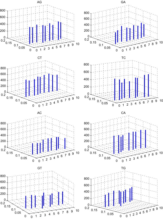
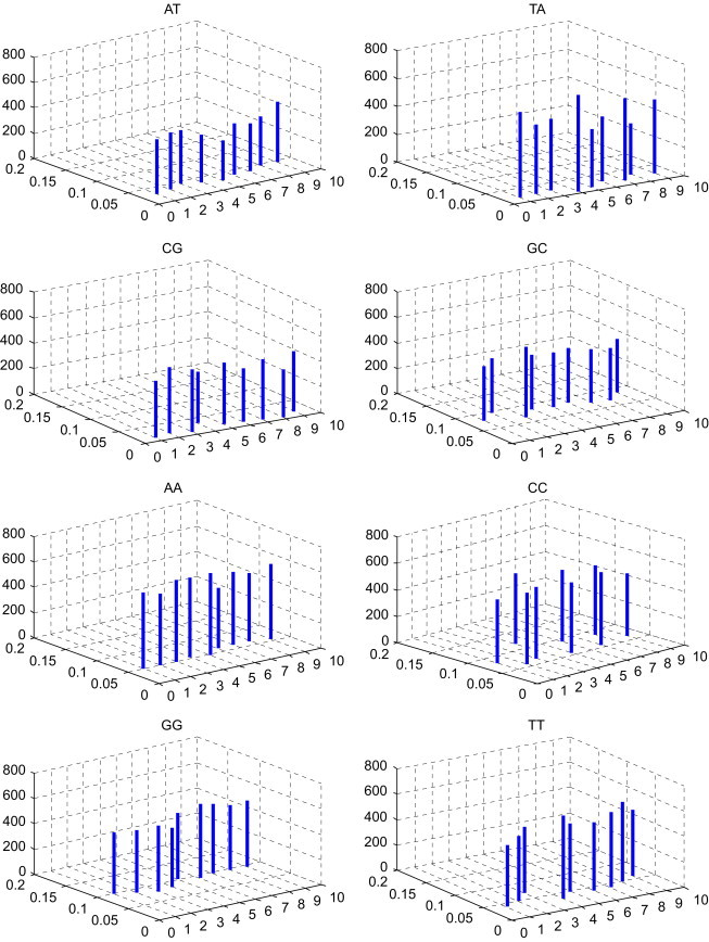
The comparison of the mean spaces and the distributions of DNs among the nine species in Table 2; i of x-coordinate denotes the ith species in Table 2, $i=1,2,\dots ,9$; the value of y-coordinate denotes the distributions of DNs; the value of z-coordinate denotes the mean spaces of DNs.

4. Similarities/dissimilarities among the complete coding sequences of $\beta$-globin gene of different species

In this section, we will illustrate the use of the quantitative characterization of DNA sequences by an examination of similarities/dissimilarities among the nine complete coding sequences in Table 2. The analysis of similarity/dissimilarity between two DNA sequences represented by the vectors is based on the assumption that the two sequences are similar if the corresponding vectors point to a similar direction and have similar magnitudes. Similar assumption is done in Randic et al. (2001).

In order to facilitate the quantitative comparison of different species, we extract some invariants with simple methods. Firstly, we calculate the space-sum matrix (s-M) as follows:

$$s\text{-}M=\left(\begin{array}{cccc}\hfill d^{\mathit{AG}}\hfill & \hfill d^{\mathit{GA}}\hfill & \hfill d^{\mathit{CT}}\hfill & \hfill d^{\mathit{TC}}\hfill \\ \hfill d^{\mathit{AC}}\hfill & \hfill d^{\mathit{CA}}\hfill & \hfill d^{\mathit{GT}}\hfill & \hfill d^{\mathit{TG}}\hfill \\ \hfill d^{\mathit{AT}}\hfill & \hfill d^{\mathit{TA}}\hfill & \hfill d^{\mathit{CG}}\hfill & \hfill d^{\mathit{GC}}\hfill \\ \hfill d^{\mathit{AA}}\hfill & \hfill d^{\mathit{CC}}\hfill & \hfill d^{\mathit{GG}}\hfill & \hfill d^{\mathit{TT}}\hfill \end{array}\right)\text{.}$$

The element $d^{\mathit{ab}}$ of the matrix s-M reveals the total sum of geometrical lengths of edges between vertices (dots) $V_1$ and all $V_{\mathit{ab}}$ of the 3D-DN curve, where $d^{\mathit{ab}}={\sum }_{k=1}^{K^{\mathit{ab}}}{d}_k^{\mathit{ab}}$, $a\in \{A,C,G,T\}$, $b\in \{A,C,G,T\}$. Similarly, we have the distribution matrix (p-M) as follows:

$$p\text{-}M=\left(\begin{array}{cccc}\hfill p^{\mathit{AG}}\hfill & \hfill p^{\mathit{GA}}\hfill & \hfill p^{\mathit{CT}}\hfill & \hfill p^{\mathit{TC}}\hfill \\ \hfill p^{\mathit{AC}}\hfill & \hfill p^{\mathit{CA}}\hfill & \hfill p^{\mathit{GT}}\hfill & \hfill p^{\mathit{TG}}\hfill \\ \hfill p^{\mathit{AT}}\hfill & \hfill p^{\mathit{TA}}\hfill & \hfill p^{\mathit{CG}}\hfill & \hfill p^{\mathit{GC}}\hfill \\ \hfill p^{\mathit{AA}}\hfill & \hfill p^{\mathit{CC}}\hfill & \hfill p^{\mathit{GG}}\hfill & \hfill p^{\mathit{TT}}\hfill \end{array}\right)\text{.}$$

The element $p^{\mathit{ab}}$ in the matrix p-M indicates the distribution of DNs on the 3D-DN curve.

We will illustrate the use of the 3D quantitative characterization of DNA sequences with an examination of similarities/dissimilarities among the nine complete coding sequences listed in Table 2. We construct two 16-component vectors (s-vector, p-vector): s-vector consisting of the 16 space-sums in the matrix s-M; p-vector consisting of the 16 distributions in the matrix p-M. Based on the assumption of similarity/dissimilarity between two DNA sequences, the similarities among such vectors can be computed in two ways: (1) calculating the Euclidean distance between the end point of the s-vectors; (2) calculating the Euclidean distance between the end point of the p-vectors. When comparing two DNA sequences, we suppose that there are two species $G_1$ and $G_2$, the parameters i and j denote row number and column number of $4\times 4$ matrix, respectively. The distance $D(G_1,G_2)$ between the two s-vectors is

$$D(G_1,G_2)={\left[\sum _{i=0}^3\sum _{j=0}^3(d_{\mathit{ij}}^{G_1}-d_{\mathit{ij}}^{G_2}{)}^2\right]}^{1/2}\text{.}$$

The distance $P(G_1,G_2)$ between the two p-vectors is

$$P(G_1,G_2)={\left[\sum _{i=0}^3\sum _{j=0}^3(p_{\mathit{ij}}^{G_1}-p_{\mathit{ij}}^{G_2}{)}^2\right]}^{1/2}\text{.}$$

The smaller the Euclidean distance is, the more similar the DNA sequences are. We list the similarities and dissimilarities for the nine complete coding sequences in Table 4, Table 5 .

Table 4.

The similarity/dissimilarity matrix for the complete coding sequences of Table 2 based on the Euclidean distances between the end points of the 16-component vectors of the space-sums of 16 DNs

Species	Human	Goat	North American opossum	Gallus	Black lemur	House mouse	Rabbit	Norway rat	Cattle
Human	0	8160	11 877	14 923	7077	8683	5874	8801	10 650
Goat		0	7790	17 978	8224	12 258	9379	10 704	5732
North American opossum			0	18 830	11 643	13 728	11 886	8483	6705
Gallus				0	18 706	11 792	17 419	14 367	20 194
Black lemur					0	12 323	5636	10 983	9938
House mouse						0	10 992	8422	13 848
Rabbit							0	9813	10 067
Norway rat								0	10 173
Cattle									0

Table 5.

The similarity/dissimilarity matrix for the complete coding sequences of Table 2 based on the Euclidean distances between the end points of the 16-component vectors of the distributions of the 16 DNs

Species	Human	Goat	North American opossum	Gallus	Black lemur	House mouse	Rabbit	Norway rat	Cattle
Human	0	0.0398	0.0480	0.0713	0.0320	0.0311	0.0348	0.0358	0.0442
Goat		0	0.0474	0.0857	0.0345	0.0442	0.0430	0.0519	0.0243
North American opossum			0	0.0834	0.0424	0.0522	0.0453	0.0450	0.0416
Gallus				0	0.0834	0.0559	0.0853	0.0715	0.0900
Black lemur					0	0.0509	0.0265	0.0547	0.0415
House mouse						0	0.0515	0.0253	0.0479
Rabbit							0	0.0525	0.0450
Norway rat								0	0.0468
Cattle									0

Observing Table 4, Table 5, we find Gallus and Opossum are very dissimilar to others among the nine species because their corresponding rows have larger entries. On the other hand, the most similar species pairs are Human–Rabbit, Goat–Cattle and Black lemur–Rabbit. The more similar species pairs are Human–Goat, House mouse–Norway rat, Human–Black lemur, Goat–North American opossum and North American opossum–Cattle. This is not an accident, but indicates that they have close evolutionary relationship. For comparison, we denote the degree of similarity of the pair Human–Gallus as 1. Then we list the above results of the examination of the degree of similarity between human and other several species in Fig. 3 . As one can see there is an overall agreement among similarity between human and other several species in Fig. 3. But the results for species 5 and 6 for methods a and b show divergent trends. We think that different invariants derived from the same 3D-DN curve bring about the divergent trends. The method a (i.e. s-vector or matrix s-M) includes the distribution information and the position information hidden in DNs of the 3D-DN curve. However, the method b (i.e. p-vector or matrix p-M) only reveals the distribution information of DNs of the 3D-DN curve. Even in Fig. 3 the emergence of the results for species 5 and 6 for methods a and b is remarkable but not for other species. The method a with more biological information, we believe, is relatively more credible than method b.

Fig. 3.

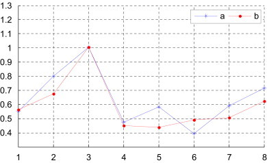
The degree of similarity of the complete coding sequences of several species with the complete coding sequence of human (a: from [this work, Table 4]; b: from [this work, Table 5]); i of x-coordinate denotes the species of Table 4 (x-coord 1: Goat, x-coord 2: North American opossum, x-coord 3: Gallus, x-coord 4: Black lemur, x-coord 5: House mouse, x-coord 6: Rabbit, x-coord 7: Norway rat, x-coord 8: Cattle).

5. Discussion

In this paper we arrange 16 DNs in a $4\times 4$ matrix according to the four categories. The matrix M is

$$\left[\begin{array}{cccc}\hfill \mathrm{AG}\hfill & \hfill \mathrm{GA}\hfill & \hfill \mathrm{CT}\hfill & \hfill \mathrm{TC}\hfill \\ \hfill \mathrm{AC}\hfill & \hfill \mathrm{CA}\hfill & \hfill \mathrm{GT}\hfill & \hfill \mathrm{TG}\hfill \\ \hfill \mathrm{AT}\hfill & \hfill \mathrm{TA}\hfill & \hfill \mathrm{CG}\hfill & \hfill \mathrm{GC}\hfill \\ \hfill \mathrm{AA}\hfill & \hfill \mathrm{CC}\hfill & \hfill \mathrm{GG}\hfill & \hfill \mathrm{TT}\hfill \end{array}\right]\text{.}$$

From the construction of the $4\times 4$ matrix, we know that their designs are not unique. There are 16 kinds of DNs, so they have $16!$ combinations. Similarly, we find out the same phenomenon in Randic (2000) and Liu et al. (2006). Randic (2000) think that the ordering of the nucleic bases in his matrix is not important. Liu et al. (2006) only consider an ordering matrix to illustrate their method.

We suggest a novel approach based on DNs to compute parameters to determine similarity/dissimilarity between two DNA sequences. The ordering of the nucleic bases in our matrix is not important. But we want to know whether the ordering of the DNs of the matrix brings about divergent trends in computing parameters to determine similarity/dissimilarity between two DNA sequences. So we randomly arrange 16 DNs in another $4\times 4$ matrix $M^{\prime }$ as follows:

$$\left[\begin{array}{cccc}\hfill \mathrm{GC}\hfill & \hfill \mathrm{GG}\hfill & \hfill \mathrm{GT}\hfill & \hfill \mathrm{TC}\hfill \\ \hfill \mathrm{TT}\hfill & \hfill \mathrm{CA}\hfill & \hfill \mathrm{AT}\hfill & \hfill \mathrm{AA}\hfill \\ \hfill \mathrm{CT}\hfill & \hfill \mathrm{TA}\hfill & \hfill \mathrm{CG}\hfill & \hfill \mathrm{AG}\hfill \\ \hfill \mathrm{TG}\hfill & \hfill \mathrm{CC}\hfill & \hfill \mathrm{GA}\hfill & \hfill \mathrm{AC}\hfill \end{array}\right]\text{.}$$

Every element of the matrix has a corresponding index $(i,j)$, $i=0,1,2,3$; $j=0,1,2,3$. Based on the index, we assign one DN as follows:

$$(0,0,0)\to \mathrm{GC},(0,1,0)\to \mathrm{GG},(0,2,0)\to \mathrm{GT},(0,3,0)\to \mathrm{TC}\text{,}(1,0,0)\to \mathrm{TT},(1,1,0)\to \mathrm{CA},(1,2,0)\to \mathrm{AT},(1,3,0)\to \mathrm{AA}\text{,}(2,0,0)\to \mathrm{CT},(2,1,0)\to \mathrm{TA},(2,2,0)\to \mathrm{CG},(2,3,0)\to \mathrm{AG}\text{,}(3,0,0)\to \mathrm{TG},(3,1,0)\to \mathrm{CC},(3,2,0)\to \mathrm{GA},(3,3,0)\to \mathrm{AC}\text{.}$$

Based on the above designation we can draw another 3D-DN curve to represent the same DNA sequence, which is named as $C^{\prime }$.

For comparison, we list the similarities and dissimilarities for the nine complete coding sequences in Table 6 by using the s-vector derived from the new 3D-DN curve $C^{\prime }$ based on the new random matrix $M^{\prime }$. As one can see there is an overall agreement among similarities obtained by different methods, despite some variation of numerical value among them. The variation of numerical value is not important. It is important whether there exit divergent trends in computing parameters to determine similarity/dissimilarity between two DNA sequences. We list the results of the examination of the degree of similarity between human and other several species in Fig. 4 . According to the results of the examination of Fig. 4 we can draw a conclusion that there exit the same trends in computing parameters to determine similarity/dissimilarity between two DNA sequences by using the s-vectors derived from different 3D-DN curves. The ordering of the nucleic bases in the suggested approach is not important.

Table 6.

The similarity/dissimilarity matrix for the complete coding sequences of Table 2 based on the Euclidean distances between the end points of the 16-component vectors of the space-sums of 16 DNs (by using the s-vector derived from the new 3D-DN curve $C^{\prime }$ based on the new random matrix $M^{\prime }$)

Species	Human	Goat	North American opossum	Gallus	Black lemur	House mouse	Rabbit	Norway rat	Cattle
Human	0	10 379	12 545	19 172	9210	10 814	7897	9602	12 403
Goat		0	8054	20 541	11 125	13 402	10 123	12 887	6669
North American opossum			0	19 740	13 302	14 171	12 391	9086	8976
Gallus				0	21 693	11 952	20 071	16 045	23 525
Black lemur					0	15 087	6044	13 759	13 335
House mouse						0	13 184	9340	16 032
Rabbit							0	10 148	11 375
Norway rat								0	14 140
Cattle									0

Fig. 4.

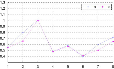
The degree of similarity of the complete coding sequences of several species with the complete coding sequence of human (a: from [this work, Table 4]; c: from [this work, Table 6]); i of x-coordinate denotes the species of Table 4 (x-coord 1: Goat, x-coord 2: North American opossum, x-coord 3: Gallus, x-coord 4: Black lemur, x-coord 5: House mouse, x-coord 6: Rabbit, x-coord 7: Norway rat, x-coord 8: Cattle).

6. Conclusion

In this paper, we give a novel approach to graphically characterize DNA primary sequences. The properties of DNs in a DNA sequence based on the $4\times 4$ matrix consisting of 16 DNs are presented in the 3D graphical representation. Based on this representation, we construct two 16-component vectors and employ the vectors in characterizing and comparing the complete coding sequence part of beta globin gene of nine different species. The results of examination show that our method is useful for visualizing the local and global features of long or short DNA sequences and can reveal the visual characteristic in a DNA sequence. The advantage of our approach is that it allows visual inspection of DNs data, helping in recognizing major similarities among different DNA sequences.

References

- Althaus I.W., Chou J.J., Gonzales A.J., Diebel M.R., Chou K.C., Kezdy F.J., Romero D.L., Aristoff P.A., Tarpley W.G., Reusser F. Biochemistry. 1993;32:6548. doi: 10.1021/bi00077a008. [DOI] [PubMed] [Google Scholar]
- Althaus I.W., Chou J.J., Gonzales A.J., Diebel M.R., Chou K.C., Kezdy F.J., Romer D.L., Aristoff P.A., Tarpley W.G., Reusser F. J. Biol. Chem. 1993;268:6119. [PubMed] [Google Scholar]
- Althaus I.W., Gonzales A.J., Chou J.J., Diebel M.R., Chou K.C., Kezdy F.J., Romero D.L., Aristoff P.A., Tarpley W.G., Reusser F. J. Biol. Chem. 1993;268:14875. [PubMed] [Google Scholar]
- Chou K.C. J. Biol. Chem. 1989;264:12074. [PubMed] [Google Scholar]
- Chou K.C. Biophys. Chem. 1990;35:1. doi: 10.1016/0301-4622(90)80056-d. [DOI] [PubMed] [Google Scholar]
- Chou K.C. J. Math. Chem. 1993;12:97. [Google Scholar]
- Chou K.C., Forsen S. Biochem. J. 1980;187:829. doi: 10.1042/bj1870829. [DOI] [PMC free article] [PubMed] [Google Scholar]
- Chou K.C., Liu W.M. J. Theor. Biol. 1981;91:637. [Google Scholar]
- Chou K.C., Zhang C.T. AIDS Res. Hum. Retrovirus. 1992;8:1967. doi: 10.1089/aid.1992.8.1967. [DOI] [PubMed] [Google Scholar]
- Chou K.C., Jiang S.P., Liu W.M., Fee C.H. Sci. Sin. 1979;22:341. [Google Scholar]
- Chou K.C., Zhang C.T., Elrod D.W. J. Protein Chem. 1996;15:59. doi: 10.1007/BF01886811. [DOI] [PubMed] [Google Scholar]
- King E.L., Altman C. J. Phys. Chem. 1956;60:1375. [Google Scholar]
- Kuzmic P., Ng K.Y., Heath T.D. Anal. Biochem. 1992;200:68. doi: 10.1016/0003-2697(92)90278-f. [DOI] [PubMed] [Google Scholar]
- Liao B., Wang T.M. Chem. Phys. Lett. 2004;338:195. [Google Scholar]
- Lin S.X., Neet K.E. J. Biol. Chem. 1990;265:9670. [PubMed] [Google Scholar]
- Liu X.Q., Dai Q., Xiu Z.L., Wang T.M. J. Theor. Biol. 2006;243:555. doi: 10.1016/j.jtbi.2006.07.018. [DOI] [PubMed] [Google Scholar]
- Nandy A. Curr. Sci. 1994;66:309. [Google Scholar]
- Nandy A., Nandy P. Chem. Phys. Lett. 2003;368:102. [Google Scholar]
- Nandy, A., Harle, M., Basak, S.C., 2006. ARKIVO, ix, 211.
- Qi Z.H., Fan T.R. Chem. Phys. Lett. 2007;442:434. [Google Scholar]
- Qi Z.H., Qi X.Q. Chem. Phys. Lett. 2007;440:139. [Google Scholar]
- Randic M. J. Chem. Inf. Comput. Sci. 2000;40:50. doi: 10.1021/ci990084z. [DOI] [PubMed] [Google Scholar]
- Randic M., Vracko M. J. Chem. Inf. Comput. Sci. 2000;40:599. doi: 10.1021/ci9901082. [DOI] [PubMed] [Google Scholar]
- Randic M., Guo X.F., Basak S.C. J. Chem. Inf. Comput. Sci. 2001;41:619. doi: 10.1021/ci000120q. [DOI] [PubMed] [Google Scholar]
- Randic M., Vracko M., Lers N., Plavsic D. Chem. Phys. Lett. 2003;371:202. [Google Scholar]
- Wang M., Yao J.S., Huang Z.D., Xu Z.J., Liu G.P., Zhao H.Y., Wang X.Y., Yang J., Zhu Y.S., Chou K.C. Med. Chem. 2005;1:39. doi: 10.2174/1573406053402505. [DOI] [PubMed] [Google Scholar]
- Wu Y.H., Liew A., Wee-C, Yan H., Yang M.S. Chem. Phys. Lett. 2003;367:170. [Google Scholar]
- Xiao X., Shao S., Ding Y., Huang Z., Chen X., Chou K.C. Amino Acids. 2005;28:29. doi: 10.1007/s00726-004-0154-9. [DOI] [PMC free article] [PubMed] [Google Scholar]
- Xiao X., Shao S., Ding Y., Huang Z., Chen X., Chou K.C. J. Theor. Biol. 2005;235:555. doi: 10.1016/j.jtbi.2005.02.008. [DOI] [PubMed] [Google Scholar]
- Xiao X., Shao S.H., Ding Y.S., Huang Z.D., Chou K.C. Amino Acids. 2006;30:49. doi: 10.1007/s00726-005-0225-6. [DOI] [PMC free article] [PubMed] [Google Scholar]
- Xiao X., Shao S.H., Chou K.C. Biochem. Biophys. Res. Commun. 2006;342:605. doi: 10.1016/j.bbrc.2006.01.166. [DOI] [PubMed] [Google Scholar]
- Zhang Y.S., Chen W. J. Theor. Biol. 2006;242:382. doi: 10.1016/j.jtbi.2006.03.012. [DOI] [PubMed] [Google Scholar]
- Zhang C.T., Chou K.C. J. Mol. Biol. 1994;238:1. doi: 10.1006/jmbi.1994.1263. [DOI] [PubMed] [Google Scholar]
- Zhang C.T., Zhang R. Nucleic Acids Res. 1991;19:6313. doi: 10.1093/nar/19.22.6313. [DOI] [PMC free article] [PubMed] [Google Scholar]
- Zhou G.P., Deng M.H. Biochem. J. 1984;222:169. doi: 10.1042/bj2220169. [DOI] [PMC free article] [PubMed] [Google Scholar]