

Highlights
-
•
Introduced vortex structure to deconstruct the airflow in the cabin.
-
•
Investigated the “lock” phenomenon for contaminants released in the vorticity.
-
•
Analyzed effects of thermal buoyancy on the contaminant longitudinal transmission.
Keywords: Aircraft cabin, Airflow vortex structure, Ventilation efficiency, Airborne contaminant transmission, Thermal buoyancy
Abstract
Airborne contaminants such as pathogens, odors and CO2 released from an individual passenger could spread via air flow in an aircraft cabin and make other passengers unhealthy and uncomfortable. In this study, we introduced the airflow vortex structure to analyze how airflow patterns affected contaminant transport in an aircraft cabin. Experimental data regarding airflow patterns were used to validate a computational fluid dynamics (CFD) model. Using the validated CFD model, we investigated the effects of the airflow vortex structure on contaminant transmission based on quantitative analysis. It was found that the contaminant source located in a vorticity-dominated region was more likely to be “locked” in the vortex, resulting in higher 62% higher average concentration and 14% longer residual time than that when the source was on a deformation dominated location. The contaminant concentrations also differed between the front and rear parts of the cabin because of different airflow structures. Contaminant released close to the heated manikin face was likely to be transported backward according to its distribution mean position. Based on these results, the air flow patterns inside aircraft cabins can potentially be improved to better control the spread of airborne contaminant.
1. Introduction
As an increasing number of people are traveling by air, the exposure risk of infectious diseases in aircraft cabins has become an important public health issue [1]. Most modern aircrafts have high-efficiency particulate air (HEPA-type) filter in their ventilation recirculation systems, which can remove more than 99.9% of the pathogen particles produced by the passengers [2]. However, these pathogen particles can spread in the cabin air before being removed by the HEPA filters. The worldwide spread of severe acute respiratory syndrome (SARS) [3] and tuberculosis (TB) [1] further indicates that the transmission of infectious diseases through airflow inside aircrafts is a key factor for passenger exposure risk. The present standards [4], [5] in commercial aircrafts provide ventilation and contaminant requirements based on the comfort of passengers. For example, ASHRAE [4] recommends a minimum air supply of 9.4 L/s per person and required the in-flight ozone concentration shall not exceed 0.25 ppm at any time. However, they do not consider the effects of airflow patterns on airborne contaminant transport. Therefore, it is important to study how aircraft cabin air flow patterns affect the transmission of airborne contaminants in the aircraft cabin to optimize the ventilation system and control the spread of infectious diseases.
Some studies have investigated the impact of airflow on airborne contaminant transmission. Table 1 shows a summary of the research in the past decade. These previous studies contribute to our understanding of airborne contaminant transmission inside aircraft cabins. They found contaminants released at points farther from the cabin exhausts had a wider spread than those released close to the exhausts, lateral dispersion in the middle injection case was more rapid than that in the side injection case due to the center mixing zone, and droplets were more likely to travel backward because of the thermal plume from infected passengers. However, they primarily focused on qualitative analysis of the bulk airflow patterns and did not consider the impact of fine airflow structures on the transmission of airborne contaminants. Recently, Li et al. [7] studied the effect of different contaminant sources and found that in the narrow cabin space, a small different (10 cm) in the source locations can result in a significant difference in contaminant fields. This indicated the fine and complex airflow structure was an important factor in determining airborne contaminant distributions.
Table 1.
Studies on airborne contaminant transmission in aircraft cabins.
| Reference | Type and facility | Occupancy | Gas/aerosol | Research data |
|---|---|---|---|---|
| Yan et al. [5] | Num. and Exp.: 5 rows, 35 seats, 2 aisles cabin mockup | 35 unheated manikins as passengers | CO2 | Simulation and measurement of airflow and gaseous contaminant |
| Sze To et al. [6] | Exp.: 3 rows, 21 seats, 2 aisles cabin mockup | 15 heated cylinders (60 W each) as passengers | Polydispersed aerosol | Dispersion and deposition of expiratory aerosols with different diameters |
| Zhang et al. [7] | Num. and Exp.: 4 rows, 28 seats, 2 aisles cabin mockup | 14 heated boxes (83 W each) as passengers | SF6 and monodispersed aerosol | Measured and predicted contaminant distributions |
| Gupta et al. [8] | Num.: 7 rows, 49 seats, 2 aisles cabin mockup | 49 heated manikins as passengers | Monodispersed aerosol | Transient spread of expiratory droplets |
| Mazumdar [9] | Num.: 15 rows, 90 seats, single aisle cabin mockup; Exp.: Reduced-scale mockup | 90 heated boxes as passengers; moving plastic box | Tracer gas; Uranine (C20H10O5S2Na) | Effects of the moving body and thermal plume on contaminant transport |
In this study, we first use experimental data from particle image velocimetry (PIV) measurement to validate the CFD model. Then, we introduce vortex structure analysis, which is a technique commonly used in studies on oceanic transmission, into the cabin environment. For example, Okubo [8] classified the two-dimensional velocity field into five parts by the roots of the characteristic equation and found that particles in different parts displayed different dispersion performances. Provenzale [9] reviewed the transmission properties of coherent vortices in rotating barotropic flows and reported that “passive tracers can be trapped inside vortex cores for long times and are transported by the vortex motion over large distances”. Isern-Fontanet et al. [10] used a common definition of a coherent structure [8], [11] to investigate the statistical vortex properties of the Mediterranean Sea. They considered this definition appropriate to identify the characteristic of vortex structure, such as size, amplitude and mean kinetic energy.
Based on the vortex structure analysis, ventilation efficiency scales for sources under different vortex structures were analyzed in cross section, and effects of the vortex structures on the contaminant longitudinal transport are investigated and compared with experimental data. This study will improve our understanding of airborne contaminant transmission in enclosed spaces and can be further developed as a strategy for controlling contaminant spreading in aircrafts.
2. Aircraft cabin and the air distribution system
A full scale aircraft cabin mockup based on the Boeing 737–200 was used for the experiment. The geometry model of the mockup is shown in Fig. 1 . The dimensions of the mockup cabin are 5.8 m (L) × 3.25 m (W) × 2.15 m (H), and it includes seven cross sections (1–7) and six longitudinal sections (A–F). The fore-wall and side-wall of the three middle rows were transparent, through which a laser can be shot into the cabin for PIV measurement [12]. Forty-two heated manikins were placed in the mockup cabin. They were wrapped with resistance wire to simulate thermal buoyancy plumes generated by passengers, and the sensible heat production for each was controlled at 75 W, simulating an actual person. Outside the mockup cabin, a chamber in which the temperature can be controlled with an error of ±1 °C was used to ensure a stable thermal boundary condition for the mockup cabin.
Fig. 1.
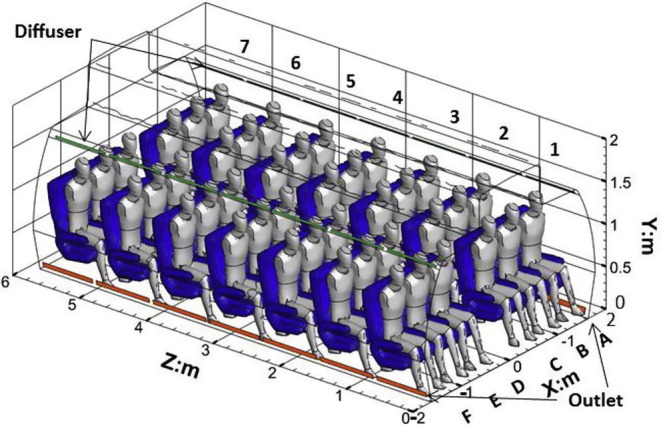
Digital geometry model of the 7-row aircraft cabin mockup.
Similar to an actual aircraft, air was supplied with overhead grille diffusers on the top of each side and was exhausted through the outlets located on each side near the floor. The supply air temperature was set at 20 °C with an error of ±0.5 °C and supply air rate was set at 9.4 L/(person·s). These values were recommended by the American Society of Heating, Refrigerating, and Air-Conditioning Engineers (ASHRAE [4]).
3. Methodology
3.1. Numerical method
3.1.1. Turbulence model and discretization schemes
In our study, we applied Reynolds-averaged Navier–Stokes (RANS) equations with the renormalization group (RNG) k–ε model [13] to calculate the airflow and turbulence recommended by Zhang et al. [14] and Zhang et al. [15]. In their reports, the predicted airflow velocity and concentration values in the cabin agreed well with experimental results. The governing equation of the RNG k-ε model is written in a general form:
| (1) |
where is the flow variables (velocity, enthalpy, turbulence parameters and mass fraction), is the effective diffusion coefficient, and is the source term. In addition, is the Reynolds-averaged velocity vector and t is time. Details about coefficients and for different variables can be found in in the Ansys theory guide [16].
Based on Eq. (1), the species transport equation can be written as:
| (2) |
where C is the local mass fraction, is the turbulent dynamic viscosity, D is the mass diffusion coefficient, and is the turbulent Schmidt number. The default of is 0.7 or 0.9 in most numerical simulations [17], but actually it differs in different conditions [17], [18]. Therefore, in this study, the number is expressed as a function of the relative kinematic viscosity [19]:
| (3) |
where is the laminar kinematic viscosity and Sc is the laminar Schmidt number.
In addition, the enhanced wall treatment [20], [21], [22] was adopted for this study because the calculated y plus value was less than five. The Boussinesq approximation was employed to consider the buoyancy effect which has been a common approach for indoor airflow simulations. For the steady velocity field simulation, this study applied the SIMPLE algorithm to couple pressure and velocity. The standard and first-order upwind scheme was used for pressure discretization and all other variables. The residual was below 10−6 for energy and 10−3 for all other variables. A commercial software Fluent was used as the numerical solver to fulfill the models.
3.1.2. Boundary conditions and grid independence test
Fig. 1 shows the overall digital geometry model. The modeled shapes of the cabin and manikins were built to the exact same dimensions as their actual physical shapes for the simulation. According to a previous study [23], we measured the velocity boundary of the diffusers by combination of hot-sphere anemometers (HSA) and ultrasonic anemometers (UA). The thermal boundary of the walls and manikins was measured by an infrared camera. The velocity and temperature boundary conditions were assigned into the numerical solver through user-defined functions (UDFs). The pressure outlet boundary condition was applied on the exhausts, and the reference pressure value was set to 0 Pa. The details of the tested velocity and temperature boundary conditions can be found in Li et al. [24].
The software ANSYS ICEM was employed to generate the meshes. Li et al. [24] did the grid convergence test for the meshes of 7-row aircraft cabin mockup. A grid convergence index (GCI) [25], [26] was calculated to show the relative error.
| (4) |
where r is the ratio of the amount of the fine grids to that of coarse grids, and is the root mean square between the values calculated by fine and coarse grids. They suggested nine million meshes were fine enough for the numerical calculation. Finally, nine million meshes for the 7-row aircraft cabin mockup were used in this study.
3.1.3. Validation of the numerical method
Li et al. [24] compared the experimental data of the airflow, temperature and sulfur hexafluoride (SF6) concentration with the simulated results to validate the reliability of the numerical methods. They reported “the agreement between the measurement and numerical calculation is acceptable for the simulation of such complicated cabin environment”. In this study, further validation was conducted to ensure that the numerical method can capture the airflow patterns and vortex structures.
In the study of Li et al. [12], they used a high power 2D-PIV system to measure the large-scale air distributions in the cabin mockup. The systematic and statistical errors were approximately 1–2% and 3–14.5% [12]. Based on their PIV measurement, we compared the airflow patterns with the simulated results. In addition, the vortex structure was calculated according to the experimental data. Okubo [8] and Weiss [11] introduced the Okubo-Weiss parameter, Q, which is the differential of deformation and vorticity square, to identify the type of vortex structure.
For the Okubo-Weiss equation:
| (5) |
where represents stretching deformation, represents shearing deformation, and w represents vorticity as follows:
| (6) |
| (7) |
| (8) |
Fig. S1 shows the visualized physical meaning of deformation and vorticity. For our study, we used Okubo-Weiss’s Q value to identify the airflow vortex structures in the cabin. When Q > 0, deformation dominates; when Q < 0, vorticity dominates. However, in a practical application, the interval of Q is always divided into three parts by q0 (q 0 = 0.2 , where is the standard deviation of Q in the entire fluid domain). When Q > q 0, the domain is dominated by deformation; when Q < −q 0, the domain is dominated by vorticity; and when −q 0 < Q < q 0, the domain is an ambient field. According to a previous study [27], these standards can identify the airflow vortex structure for complex fluids. In this study, this standard was adopted, and the airflow vortex structures calculated through the experimental data were used to validate the CFD model as well.
Fig. 2 compares the experimental airflow patterns with corresponding simulated data. Because of the blocks of seats and manikins, only the airflow in the upper and middle domains of this section was obtained through PIV measurement. It is shown that the decay of simulated velocity seems slower than the experiment. Lin et al. [28] stated that the RANS simulation underpredicted the turbulence energy, while a large eddy simulation (LES) can obtain more realistic turbulent energy. The LES simulation needs much more meshes than nine million, and it is beyond the current computer capability. However, the simulated results agree with the experiments in the sense that the CFD model captured the trend of airflow patterns. The jets from the right and left diffusers are merged in the middle, and the jets from left sides are both little stronger. The velocity magnitudes are lower in the top and side regions.
Fig. 2.

Comparison of the experimental and simulated airflow patterns in CS4: (a) predicted airflow pattern. (b) PIV experimental airflow pattern.
Fig. 3 presents the comparison of the experimental and simulated vortex structures. The red regions in the figure are dominated by deformation, blue regions are dominated by vorticity, and the green regions are ambient fields. The simulated results seem smoother, while the experiment has more discrete points. However, the CFD model captures the two big vorticities on the sides and the domain dominated by deformation in the middle.
Fig. 3.

Comparison of the experimental and simulated vortex structures in CS4: (a) predicted vortex structure. (b) PIV experimental vortex structure.
Three indexes were employed to quantify the data comparison. They were relative root mean square error (RRMSE), correlation coefficient (r) and overall coincidence degree (). They are expressed as:
| (9) |
| (10) |
| (11) |
where are the experimental and simulated velocity at sampling point i. are the average velocity. and are the 10th and 90th velocity in all experimental data. RRMSE between the experimental and predicted data was 0.70, r was 0.86, and was 0.70, indicating that the experimental data had good correlation and overlapping with the predicted data, but the discrepancies were observable between the pairs. In such complicated cabin environment, this agreement between the experiment and prediction was acceptable.
3.2. Experimental set-up
To investigate effects of airflow vortex structures and the thermal plumes on the contaminant longitudinal transport, tracer gas (mixed SF6, 1% SF6 balanced with 99% N2) representing the aerosol contaminant was released and measured in the cabin. The tracer gas was released at a rate of 1 L/min with nearly zero momentum to avoid its effect on the airflow fields. As illustrated in Fig. 4 , three cases were conducted, and the index manikin was located at 4C (Fig. 1).
Fig. 4.

Schematic of the cases for the longitudinal transport study: (a) mouth source with heated manikins. (b) mouth source with unheated manikins. (c) forward source with heated manikins.
Case (1): Mouth source with heated manikins (Fig. 4 (a)).
In this case, the source of tracer gas was set at the mouth of the manikin, and all manikins in the cabin were heated. This case represented a normal condition.
Case (2): Mouth source with unheated manikins (Fig. 4(b)).
In this case, all manikins were unheated. All other boundary settings were exactly the same as those in Case (1). Thus, Case (2) was designed to reflect the impact of thermal plumes from the manikins.
Case (3): Forward mouth source with heated manikins (Fig. 4(c)).
In this case, the source was moved forward with 20 cm. All other boundary settings were exactly the same as those in Case (1). Thus, Case (3) was used to further investigate the impact of different vortex structures induced by the thermal plumes on contaminant longitudinal transport.
To analyze longitudinal transport trends of the contaminant, the concentrations of row 1 and 7 were measured. Four sampling points were set at the outlets of row 1 and 7, because the concentration of outlet can represent the well mixed value at this row. In addition, sampling time of each point was set to be one 3 ( is the time constant which is the volume of the cabin divided by ventilation rate, and is 80 s in this study). This is because, under the hypotheses of well mixed, the air in a cabin can be exchanged fully after 3 [29]. From Ott [30], the concentration distribution at a sampling point can be regard as a product of many independent, successive and random dilution of an initial concentration, which is log-normal. Therefore, for each point data series, its geometric average and standard deviation were calculated for analysis [31].
4. Results
4.1. Contaminant transport in the cross section
As discussed in Section 3.1.3, we could obtain reliable airflow patterns and vortex structures through the CFD simulation. This CFD model was employed to investigate the effects of airflow vortex structures on airborne contaminant transmission. Three sources were set according to the vortex distribution (Fig. 5 (a)). Source 2 is in the middle region dominated by deformation, and source 1 and 3 are on the sides dominated by vorticity. Rather than the vortex structure, the relative distances between the sources and inlet/outlet could also affect the airborne contaminant distribution [6]. Therefore, these adjacent sources were a distance of only 10 cm apart. The contaminant distributions for these three sources were compared.
Fig. 5.

(a) Vortex structure in the cross section. Predicted concentration and path lines for: (b) source 1(c) source 2 (d) source 3.
From Fig. 5, these three sources with closed distance but different vortex structures led to observable different concentration distributions. The contaminants from source 2 seem be delivered to the cabin bottom and exhausted directly. Few of them can spread to the upsides of the cabin (Fig. 5(c)). In contrast to source 2, the contaminants from source 1 and 3 can be transported to its respective upside, and the concentration above the seats is much higher (Fig. 5(a, d)). Using a path line as an indicator, the trajectory of the contaminant can be indicated more clearly. In this section, 20 massless particles [16] were released on each location, and their trajectories were got. The path lines from source 2 almost escaped from the cabin, and fewer path lines went back to the upsides (Fig. 5(c)). However, more path lines from source 1 and 3 were recirculated back to the upsides, which resulted in higher concentrations above the seats (Fig. 5(a,d)). This meant the region dominated by vorticity had a “lock” function which could lock the contaminant inside and make it difficult to escape.
Mean positions of contaminants can be used to identify their distribution difference [32]. The predicted mean position can be determined by the following method: multiply the simulated concentration by the position x, y or z depending on the analysis plane, sum the value for all points, and then divide the sum by the total value of concentration. Table. 2 shows the mean positions for different cases. From the upper part of Table. 2, the distances between the mean positions are much larger than their source positions, indicating that the different vortex structures lead to observable different concentration distributions.
Table 2.
Mean positions of the predicted contaminant distributions.
| Position (x,y) | Source |
||
|---|---|---|---|
| 1 Source | 2 Source | 3 Source | |
| Contaminant transport in the cross section | |||
| Source position (m) | (−0.04, 0.8) | (0.06, 0.8) | (0.16, 0.8) |
| Mean position (m) | (−0.15, 0.59) | (0.25, 0.58) | (0.44, 0.68) |
| Position (y,z) | Source | ||
| Mouth source | Forward source | ||
| Contaminant transport in the longitudinal section | |||
| Source position (m) | (1.2, 2.83) | (1.2, 2.63) | |
| Mean position (m) | (1.06, 2.84) | (1.08, 2.59) | |
Dimensionless average concentration (DAC), contaminant transmission radius (CTR) and residual time of the air (RTA) from Kato and Murakami [33] were applied to further evaluate the characteristics of airborne contaminant distributions quantitatively. DAC is an index describing the dimensionless average concentration. It is defined as follows:
| (12) |
where and are the concentration (kg/m3) and volume (m3) of the computed cell, respectively, at position x when the source is at location , q is the contaminant generation rate (kg/(m3·s)), is the ventilation rate (m3/s) and V is the cabin volume. Additionally, is the integrated concentration when the source is at location and is the instantaneous uniform concentration.
CTR is an index showing the contaminant transmission radius and is defined as follows:
| (13) |
| (14) |
where is the central position of the contaminant field. The residual time of the air is the time that the contaminants released from the source spend in the cabin before being exhausted, and it can be calculated from a reversed airflow filed [33]. These indexes can be calculated in the CFD solver by UDFs.
Table 3 presents DAC, CTR and RTA for different sources. Corresponding to Fig. 5, the dimensionless average concentrations for source 1 and 3 dominated by vorticity are 62% higher than that for source 2. The residual times of the air at source 1 and 3 location are 14% longer, because the air “locked” by vorticity needs more time to escape from the cabin. However, the contaminant transmission radiuses for different sources are not observable. This maybe because most of the contaminants can be exhausted in the same row, and the transmission radius is dependent on the cross section size to a great extent.
Table 3.
DAC, CTR and RTA for different sources.
| Source | DAC | CTR (m) | RTA (s) |
|---|---|---|---|
| 1 | 0.26 | 1.11 | 31 |
| 2 | 0.17 | 1.13 | 29 |
| 3 | 0.29 | 1.12 | 35 |
4.2. Contaminant transport in the longitudinal section
Airborne contaminant transmission in the longitudinal direction was also investigated. The trends of contaminant longitudinal transmission were revealed by measuring and simulating the concentrations at the outlets (A side and F side) of row 1 and row 7. For Case (1), Fig. 6 (a) shows that the concentrations of row 1 are lower than those of row 7, and experimental and simulated data have the same trend. The error bars of experimental data present their geometric standard deviation intervals. For Case (2), in which the manikins were unheated, Fig. 6(b) shows the concentration differences between row 1 and 7 in this case were different with Case (1), and the experimental and simulated data have some discrepancy. For Case (3), the source was moved forward with 20 cm and the manikins were heated. Fig. 6(c) shows the average experimental and simulated concentrations of row 1 are both a little higher.
Fig. 6.

Comparison of the experimental and simulated concentrations at row 1 and 7 for: (a) case 1: mouth source with heated manikins, (b) case 2: mouth source with unheated manikins, (c) case 3: forward source with heated manikins.
To explain the data in Fig. 6, the velocity and vortex structure distributions on longitudinal section through source 4C were calculated. As Fig. 7 shows, the velocities in the vicinity of heated manikin are higher and dominated by the downward negative buoyancy flow, and the distinction between vorticity and deformation is observable. A white line “MN” is drawn in the mouth front region dominated by deformation. On both sides of line MN, two vortexes were captured. Ten massless particles were released on each side respectively to get their path lines. Note that path lines are three dimensional and the two dimensional figure can only show their projections. Fig. 7 suggests if a contaminant source was on the left side of line MN, the contaminants were more likely transported forward, but if the source was on the right side of line MN, the contaminants went downward and did not cross line MN. From the lower part of Table. 2, it presents clearly that, comparing with the source position, the mean position of mouth source moves back, while the mean position of forward source moves forth. This can explain why the concentration trends between row 1 and 7 was contrary when moving the source with 20 cm.
Fig. 7.

Path lines, velocity and vortex structure distributions for heated manikins.
In contrast to the velocity and vortex structure distributions for heated manikins, Fig. 8 shows, in the vicinity of unheated manikin, lower velocities and ambient field of Q value captured most of the area. From the path lines of particles, the contaminants released in this region were difficult to disperse, and the transmission in this area had much uncertainty. Corresponding to Fig. 6(b), the measured concentration has large geometric standard deviation intervals and different trend with the simulated data.
Fig. 8.

Path lines, velocity and vortex structure distributions for unheated manikins.
5. Discussion and limits of the study
In the cabin, the height of breathing zone is 1.2 m approximately, and the breathing zones are almost in vortex dominated regions (Fig. 3). According the results in Section 4.1, the contaminants from passengers are likely to be “locked” in these regions and the air quality is poor. However, the vertical flow in the middle can block the contaminant spreading to the other side. Some studies [15], [34] evaluated the performances of different ventilation systems, such as mixing ventilation, mixing ventilation combined with personal ventilation (PV), under floor ventilation and under floor ventilation combined with PV, and they found that the system can robustly prevent the airborne contaminants from entering the passenger’s breathing region by combining the ventilation system with personal air supply.
Chen et al. [35] calculated the distance that a breathing jet can travel as follows:
| (15) |
where s∗ is the distance that a breathing jet can travel, is the initial breathing velocity (m/s), is the diameter of the mouth (m), L is the distance from the mouth to the wall (m), and is the reference room air velocity (m/s). The details of these parameters can be found in Gupta et al. [36]. Through this calculation, the distance that a breathing jet could travel in our study is approximately 40 cm. Therefore, we can assume that, if a person breathes through the nose (the contaminants were released close to the face), the airborne contaminants are more likely to be transported backward. However, if a person breathes through the mouth, the breathing jet can go through line MN (Fig. 7), and therefore, the airborne contaminants are more likely to be transported forward.
Bianco et al. [37] analyzed the transient airflow behavior in the cabin. They reported observable velocity fluctuations, probably due to the flow field instability, which was caused by the vortex movements. This means the vortex structures is actually transient in the cabin. However, the current PIV experiment [12] can only capture the time-averaged airflow field. Therefore, the RANs model is appropriate in this study. With the experimental technology developing, some transient numerical models such as URANS and LES model can be used to investigate transient airflow and vortex movements.
6. Conclusions
The aim of this study was to investigate how the vortex structures of airflow affect airborne contaminant transmission in an aircraft cabin. We employed an Okubo-Weiss parameter Q from fluid mechanics to identify the vortex structures. By setting the contaminant sources at locations with different vortex structures in the simulation and experiment in the 7-row cabin, we found that the fine airflow vortex structure has an important effect on airborne contaminant distributions.
In the cross section, when the contaminants were released from a location dominated by vorticity, they were more likely to be “locked” in the vortex, resulting in 62% higher average concentration and 14% longer residual time than that when the source was on a location dominated by deformation. However, these locations should have similar relative distances to diffusers and exhausts. In the longitudinal section, different airflow vortex structures also resulted in different concentrations between the front and rear parts. The airflows close to the heated manikin’s chest and face was more likely to move contaminants backward, while the airflows distanced to it was more likely to deliver contaminants forward. However, the trend for unheated manikins was uncertainty, because of low longitudinal velocity and Q value.
This research also demonstrated that the CFD simulation could be used to investigate the mechanisms of airborne contaminant transmission in aircraft cabins, because it could provide more detailed information about the airflows and vortex structures, which were difficult to be measured by experiment. The vortex structure analysis also can not only be applied in cabin environments, but also in another enclosed environments such as rail cabins and submarines. Further research on applications of more advanced numerical models and three-dimensional vortex structure analysis are needed.
Acknowledgement
The research presented in this paper was supported financially by the National Basic Research Program of China (The 973 Program) through Grant No. 2012CB720100. The authors would like to thank for the support from the program of China Scholarships Council (No. 201306250088) and David Fung from the University of California in Los Angeles.
Footnotes
Supplementary data associated with this article can be found, in the online version, at http://dx.doi.org/10.1016/j.ijheatmasstransfer.2016.01.004.
Appendix A. Supplementary data
Schematic of the deformation and vorticity.
References
- 1.Mangili A., Gendreau M.A. Transmission of infectious diseases during commercial air travel. Lancet. 2005;365(9463):989–996. doi: 10.1016/S0140-6736(05)71089-8. [DOI] [PMC free article] [PubMed] [Google Scholar]
- 2.E.H. Hunt, D.H. Reid, D.R. Space, F.E. Tilton, Commercial airliner environmental control system, in: Aerospace Medical Association Annual Meeting, 1995.
- 3.Olsen S.J., Chang H.L., Cheung T.Y.-Y., Tang A.F.Y., Fisk T.L., Ooi S.P.L., Kuo H.W., Jiang D.D.S., Chen K.T., Lando J. Transmission of the severe acute respiratory syndrome on aircraft. N. Engl. J. Med. 2003;349(25):2416–2422. doi: 10.1056/NEJMoa031349. [DOI] [PubMed] [Google Scholar]
- 4.A. ASHRAE, Standard 161–2007, Air Quality within Commercial Aircraft, American Society of Heating, Refrigerating and Air-Conditioning Engineers, Inc, Atlanta, 2007).
- 5.F.A.R. Part, 25: Airworthiness standards: Transport category airplanes, Federal Aviation Administration, Washington, DC, 7, 2002.
- 6.Yan W., Zhang Y., Sun Y., Li D. Experimental and CFD study of unsteady airborne pollutant transport within an aircraft cabin mock-up. Build. Environ. 2009;44(1):34–43. [Google Scholar]
- 7.Li F., Liu J., Pei J., Lin C.H., Chen Q. Experimental study of gaseous and particulate contaminants distribution in an aircraft cabin. Atmos. Environ. 2014;85:223–233. doi: 10.1016/j.atmosenv.2013.11.049. [DOI] [PMC free article] [PubMed] [Google Scholar]
- 8.Okubo A. Deep Sea Research and Oceanographic Abstracts. Elsevier; 1970. Horizontal dispersion of floatable particles in the vicinity of velocity singularities such as convergences; pp. 445–454. [Google Scholar]
- 9.Provenzale A. Transport by coherent barotropic vortices. Annu. Rev.fluid Mech. 1999;31(1):55–93. [Google Scholar]
- 10.Isern-Fontanet J., Font J., García-Ladona E., Emelianov M., Millot C., Taupier-Letage I. Spatial structure of anticyclonic eddies in the Algerian basin (Mediterranean Sea) analyzed using the Okubo-Weiss parameter. Deep Sea Res. Part II: Topical Stud. Oceanogr. 2004;51(25):3009–3028. [Google Scholar]
- 11.Weiss J. The dynamics of enstrophy transfer in two-dimensional hydrodynamics. Phys. D: Nonlinear Phenom. 1991;48(2):273–294. [Google Scholar]
- 12.Li J., Cao X., Liu J., Wang C., Zhang Y. Global airflow field distribution in a cabin mock-up measured via large-scale 2D PIV. Build. Environ. 2015 [Google Scholar]
- 13.D. Choudhury, Introduction to the renormalization group method and turbulence modeling, Fluent Incorporated, 1993.
- 14.Zhang Z., Chen X., Mazumdar S., Zhang T., Chen Q. Experimental and numerical investigation of airflow and contaminant transport in an airliner cabin mockup. Build. Environ. 2009;44(1):85–94. [Google Scholar]
- 15.Zhang T.T., Li P., Wang S. A personal air distribution system with air terminals embedded in chair armrests on commercial airplanes. Build.Environ. 2012;47:89–99. [Google Scholar]
- 16.A.F. Ansys, 14.0 Theory Guide, ANSYS inc, 2011.
- 17.Tominaga Y., Stathopoulos T. Turbulent Schmidt numbers for CFD analysis with various types of flowfield. Atmos. Environ. 2007;41(37):8091–8099. [Google Scholar]
- 18.He G., Guo Y., Hsu A.T. The effect of Schmidt number on turbulent scalar mixing in a jet-in-crossflow. Int. J. Heat Mass Transfer. 1999;42(20):3727–3738. [Google Scholar]
- 19.Goldman I., Marchello J. Turbulent schmidt numbers. Int. J. Heat Mass Transfer. 1969;12(7):797–802. [Google Scholar]
- 20.Chen H., Patel V. Near-wall turbulence models for complex flows including separation. AIAA J. 1988;26(6):641–648. [Google Scholar]
- 21.Kader B. Temperature and concentration profiles in fully turbulent boundary layers. Int. J. Heat Mass Transfer. 1981;24(9):1541–1544. [Google Scholar]
- 22.Wolfshtein M. The velocity and temperature distribution in one-dimensional flow with turbulence augmentation and pressure gradient. Int. J. Heat Mass Transfer. 1969;12(3):301–318. [Google Scholar]
- 23.Liu W., Wen J., Chao J., Yin W., Shen C., Lai D., Lin C.H., Liu J., Sun H., Chen Q. Accurate and high-resolution boundary conditions and flow fields in the first-class cabin of an MD-82 commercial airliner. Atmos. Environ. 2012;56:33–44. [Google Scholar]
- 24.Li M., Zhao B., Tu J., Yan Y. Study on the carbon dioxide lockup phenomenon in aircraft cabin by computational fluid dynamics. Build. Simul. 2015;8(4):431–441. [Google Scholar]
- 25.Richardson L.F. The approximate arithmetical solution by finite differences of physical problems involving differential equations, with an application to the stresses in a masonry dam. Philos. Trans. R. Soc. London. Ser. A. 1911:307–357. [Google Scholar]
- 26.Roache P.J. Perspective: a method for uniform reporting of grid refinement studies. J. Fluids Eng. 1994;116(3):405–413. [Google Scholar]
- 27.Isern-Fontanet J., García-Ladona E., Font J. Vortices of the Mediterranean Sea: an altimetric perspective. J. Phys. Oceanogr. 2006;36(1):87–103. [Google Scholar]
- 28.Lin C., Horstman R., Ahlers M., Sedgwick L., Dunn K., Topmiller J., Bennett J., Wirogo S. Numerical simulation of airflow and airborne pathogen transport in aircraft cabins–Part I: numerical simulation of the flow field. ASHRAE Trans. 2005;111(1):755–763. [Google Scholar]
- 29.Etheridge D., Sandberg M. John Wiley & Sons Chichester; USA: 1996. Building Ventilation: Theory and Measurement. [Google Scholar]
- 30.Ott W.R. CRC Press; 1994. Environmental Statistics and Data Analysis. [Google Scholar]
- 31.Tan Y., Robinson A.L., Presto A.A. Quantifying uncertainties in pollutant mapping studies using the Monte Carlo method. Atmos. Environ. 2014;99:333–340. [Google Scholar]
- 32.Wan M., Sze To G., Chao C., Fang L., Melikov A. Modeling the fate of expiratory aerosols and the associated infection risk in an aircraft cabin environment. Aerosol Sci. Technol. 2009;43(4):322–343. [Google Scholar]
- 33.Kato S., Murakami S. New ventilation efficiency scales based on spatial distribution of contaminant concentration aided by numerical simulation. ASHRAE Trans. 1988;94:309–330. [Google Scholar]
- 34.Gao N., Niu J. Personalized ventilation for commercial aircraft cabins. J. Aircr. 2008;45(2):508–512. [Google Scholar]
- 35.Chen C., Liu W., Li F., Lin C.H., Liu J., Pei J., Chen Q. A hybrid model for investigating transient particle transport in enclosed environments. Build. Environ. 2013;62:45–54. doi: 10.1016/j.buildenv.2012.12.020. [DOI] [PMC free article] [PubMed] [Google Scholar]
- 36.Gupta J.K., Lin C.H., Chen Q. Transport of expiratory droplets in an aircraft cabin. Indoor Air. 2011;21(1):3–11. doi: 10.1111/j.1600-0668.2010.00676.x. [DOI] [PubMed] [Google Scholar]
- 37.Bianco V., Manca O., Nardini S., Roma M. Numerical investigation of transient thermal and fluidynamic fields in an executive aircraft cabin. Appl. Therm. Eng. 2009;29(16):3418–3425. [Google Scholar]
Associated Data
This section collects any data citations, data availability statements, or supplementary materials included in this article.
Supplementary Materials
Schematic of the deformation and vorticity.