Bifurcation analysis of an SIRS epidemic model with a generalized nonmonotone and saturated incidence rate

Abstract

In this paper, we study a susceptible-infectious-recovered (SIRS) epidemic model with a generalized nonmonotone and saturated incidence rate $\frac{k{I}^{2}S}{1+\beta I+\alpha I^2}$, in which the infection function first increases to a maximum when a new infectious disease emerges, then decreases due to psychological effect, and eventually tends to a saturation level due to crowding effect. It is shown that there are a weak focus of multiplicity at most two and a cusp of codimension at most two for various parameter values, and the model undergoes saddle-node bifurcation, Bogdanov-Takens bifurcation of codimension two, Hopf bifurcation, and degenerate Hopf bifurcation of codimension two as the parameters vary. It is shown that there exists a critical value $\alpha ={\alpha }_0$ for the psychological effect, and two critical values $k=k_0,k_1(k_0<k_1)$ for the infection rate such that: (i) when $\alpha >{\alpha }_0$, or $\alpha \le {\alpha }_0$ and $k\le k_0$, the disease will die out for all positive initial populations; (ii) when $\alpha ={\alpha }_0$ and $k_0<k\le k_1$, the disease will die out for almost all positive initial populations; (iii) when $\alpha ={\alpha }_0$ and $k>k_1$, the disease will persist in the form of a positive coexistent steady state for some positive initial populations; and (iv) when $\alpha <{\alpha }_0$ and $k>k_0$, the disease will persist in the form of multiple positive periodic coexistent oscillations and coexistent steady states for some positive initial populations. Numerical simulations, including the existence of one or two limit cycles and data-fitting of the influenza data in Mainland China, are presented to illustrate the theoretical results.

1. Introduction

In the classical infectious disease transmission models (Kermack and McKendrick [16], Hethcote [12]), the population is divided into three classes labeled by $S(t)$, $I(t)$ and $R(t)$, representing the numbers of susceptible, infective, and recovered or removed individuals at time t, respectively. Assuming the recovered individuals have temporary immunity, the classical susceptible-infectious-recovered (SIRS) model can be written as follows:

$$\begin{array}{cc}\hfill & \frac{dS}{dt}=b-dS-g(I)S+\delta R,\hfill \\ \hfill & \frac{dI}{dt}=g(I)S-(d+\mu )I,\hfill \\ \hfill & \frac{dR}{dt}=\mu I-(d+\delta )R,\hfill \end{array}$$ (1.1)

where b is the recruitment rate of the population, d is the natural death rate of the population, μ is the natural recovery rate of the infective individuals, δ is the rate at which recovered individuals lose immunity and return to the susceptible class. $g(I)S$ is called the incidence rate, and $g(I)$ is a function to measure the infection force of a disease.

The incidence rate $g(I)S$ plays a very important role in describing the evolution of infectious disease. In [16] Kermack and McKendrick assumed that the incidence rate is bilinear, i.e.,

$$g(I)S=kIS,$$ (1.2)

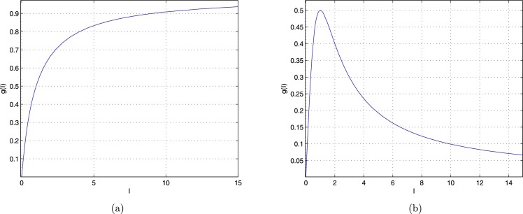
where $g(I)=kI$ is unbounded when $I\ge 0$. The bilinear incidence rate (1.2) might be true when the number of the infective individuals $I(t)$ is small, but it becomes unrealistic when $I(t)$ is getting larger. Studying the data on the cholera epidemic spread in Bari, Italy, in 1973, Capasso et al. [5] and Capasso and Serio [6] proposed two types of nonlinear incidence rates, namely a saturated incidence rate and an incidence rate taking psychological effect into account (see Fig. 1.1 ).

Fig. 1.1.

Two types of nonlinear incidence function g(I). (a) A saturated incidence function; (b) An incidence function with psychological effect.

(a) Saturated Incidence Rates. To compare with the bilinear incidence rate (1.2), Capasso and Serio [6] proposed a saturated incidence rate of the following form:

$$g(I)S=\frac{kIS}{1+\alpha I},$$ (1.3)

where kI measures the infection force of the disease and $\frac{1}{1+\alpha I}$ measures the inhibition effect from the behavioral change of the susceptible individuals when their number increases or from the crowding effect of the infective individuals (Ruan and Wang [25]). Notice that the nonlinear incidence function $g(I)$ eventually tends to a saturation level $\frac{k}{\alpha }$ when I is getting larger.

The general incidence rate

$$g(I)S=\frac{k{I}^{p}S}{1+\alpha I^q}$$ (1.4)

was proposed by Liu et al. [20] ($q=p-1$) and Hethcote and van den Driessche [13] ($p\ge q$), and used by a number of authors, see, for example, Alexander and Moghadas [1], [2], Derrick and van den Driessche [9], [10], Li et al. [17], Liu et al. [19], Lizana and Rivero [21], Moghadas and Alexande [22], and Wang [28]. According to Tang et al. [27] and Hu et al. [14], the incidence function $g(I)=\frac{k{I}^p}{1+\alpha I^q}$ includes three types: (i) unbounded incidence function: $p>q$; (ii) saturated incidence function: $p=q$; and (iii) nonmonotone incidence function: $p<q$. In order to better understand the generic bifurcations in SIRS models with saturated incidence rates, Ruan and Wang [25] studied model (1.1) with a specific nonlinear incidence rate,

$$g(I)S=\frac{k{I}^{2}S}{1+\alpha I^2},$$ (1.5)

and presented a detailed qualitative and bifurcation analysis of the model.

(b) Nonmonotone Incidence Rates with Psychological Effect. Though Capasso and Serio [6] described incidence functions taking into account psychological effect, but they did not give any specific function to describe such incidence. To model the effects of psychological factor, protection measures and intervention policies when a serious disease emerges, Xiao and Ruan [29] proposed the following specific incidence rate:

$$g(I)S=\frac{kIS}{1+\alpha I^2},$$ (1.6)

where the incidence function $g(I)=\frac{kI}{1+\alpha I^2}$ is nonmonotone when $I\ge 0$ (see Fig. 1.1(b)). This implies that the contact rate and the infection probability are increasing when a new infectious disease emerges, since people have very little knowledge about the disease. However, when I is large and the disease becomes more serious, psychological factor leads people to implementing measures to control the spread of the disease. For example, in the outbreak of severe acute respiratory syndrome (SARS), the aggressive measures and policies, such as border screening, mask wearing, quarantine, isolation, etc. were proved to be very effective in reducing the transmission. So the infection force decreases when the number of infected individuals becomes larger. Liu et al. [18] used (1.6) to describe the psychological effect toward avian influenza in the human population. In [29], Xiao and Ruan presented a global analysis for model (1.1) with nonmonotone incidence rate (1.6), and showed that either the number of infective individuals tends to zero as time evolves or the disease persists. Hence, model (1.1) with nonmonotone incidence rate (1.6) cannot exhibit complicated dynamics and bifurcations.

Xiao and Zhou [30] considered a complete form of the nonmonotone incidence rate (1.6) as follows:

$$g(I)S=\frac{kIS}{1+\beta I+\alpha I^2},$$ (1.7)

where β is a parameter such that $1+\beta I+\alpha I^2>0$ for all $I\ge 0$, hence, $\beta >-2\sqrt{\alpha }$. They presented qualitative analysis of model (1.1) with nonmonotone incidence rate (1.7) and showed the existence of bistable phenomenon and periodic oscillation. Zhou et al. [32] further studied the existence of different kinds of bifurcations, such as Hopf and Bogdanov-Takens bifurcations.

(c) Nonmonotone and Saturated Incidence Rates. Note that both nonmonotone incidence functions $\frac{kI}{1+\alpha I^2}$ and $\frac{kI}{1+\beta I+\alpha I^2}$, given in (1.6) and (1.7), tend to zero when I goes to infinite, which indicates that the psychological or inhibitory effect from the behavioral change of the susceptible individuals or from the crowding effect of the infective individuals is too strong, which may be unreasonable for some specific infectious diseases, such as influenza. Thus, a more reasonable incidence function $g(I)$ may be one that first increases to a maximum when a new infectious disease emerges or an old infectious disease reemerges, then decreases due to psychological effect, and eventually tends to a saturation level due to crowding effect. On the other hand, in some specific infectious diseases, the incidence rate may not be monotonic or non-monotonic alone, a more general incidence rate may have a combination of monotonicity, nonmonotonicity and saturation properties.

Based on the above discussions, in this paper, we propose the following general nonmonotone and saturated incidence rate:

$$g(I)S=\frac{k{I}^{2}S}{1+\beta I+\alpha I^2},$$ (1.8)

where $\alpha >0$ is a parameter which measures the psychological or inhibitory effect, and k is the infection rate. β is a parameter such that $1+\beta I+\alpha I^2>0$ for all $I\ge 0$, hence, $\beta >-2\sqrt{\alpha }$. When $\beta \ge 0$, $g(I)=\frac{k{I}^2}{1+\beta I+\alpha I^2}$ is monotonic, always increases and then tends to a saturated level $\frac{k}{\alpha }$ as I goes to infinite. When $-2\sqrt{\alpha }<\beta <0$, $g(I)$ is nonmonotonic, increases when I is small and decreases when I is large, and finally tends to a saturated level $\frac{k}{\alpha }$ as I goes to infinite (see Fig. 1.2 ). It can be seen from Fig. 1.2 that when α and k are fixed, $g(I)$ increases faster for smaller β when I is small, and then decreases to the same fixed value $\frac{k}{\alpha }$ for any β.

Fig. 1.2.

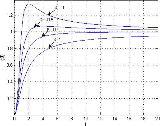
Properties of function g(I) in (1.8) for α = 1, k = 1 with β = −1,−0.5,0,1.

When $\beta =0$, the general incidence rate (1.8) becomes the saturated incidence rate (1.5). Ruan and Wang [25] studied model (1.1) with incidence rate (1.5) and presented a detailed qualitative and bifurcation analysis of the model. They showed that the system undergoes Bogdanov-Takens bifurcation of codimension two and Hopf bifurcation of codimension one, but the exact codimension of Hopf bifurcation remains unknown. In [27], Tang et al. proved that the maximal multiplicity of the weak focus is two by complex algebraic calculations but did not give the explicit conditions for degenerate Hopf bifurcation. Moreover, they claimed the existence of Bogdanov-Takens bifurcation of codimension three. They also conjectured that model (1.1) with nonmonotone incidence rate would not exhibit complicated dynamics and bifurcations.

In this paper, for the case $\beta >-2\sqrt{\alpha }$ we find that model (1.1) with general incidence rate (1.8) can exhibit complicated dynamical behaviors and bifurcation phenomena. More precisely, we will show that there are a weak focus of multiplicity at most two and a cusp of codimension at most two for various parameter values, and the model undergoes saddle-node bifurcation, Bogdanov-Takens bifurcation of codimension two, Hopf bifurcation, and degenerate Hopf bifurcation of codimension two as the parameters vary. By considering a more general model, our results show that Bogdanov-Takens bifurcation of codimension higher than two cannot occur, which clarifies and corrects the corresponding results obtained by Tang et al. [27], who claimed the existence of Bogdanov-Takens bifurcation of codimension three. Moreover, our results about degenerate Hopf bifurcation of codimension two can be seen as a complement of the results obtained by Ruan and Wang [25], who only discussed the Hopf bifurcation of codimension one. Furthermore, it is shown that there exists a critical value $\alpha ={\alpha }_0$ for the psychological or inhibitory effect, and two critical values $k=k_0,k_1(k_0<k_1)$ for the infection rate such that: (i) when $\alpha >{\alpha }_0$, or $\alpha \le {\alpha }_0$ and $k\le k_0$, the disease will die out for all positive initial populations; (ii) when $\alpha ={\alpha }_0$ and $k_0<k\le k_1$, the disease will die out for almost all positive initial populations; (iii) when $\alpha ={\alpha }_0$ and $k>k_1$, the disease will persist in the form of a positive coexistent steady state for some positive initial populations; and (iv) when $\alpha <{\alpha }_0$ and $k>k_0$, the disease will persist in the form of multiple positive periodic coexistent oscillations and coexistent steady states for some positive initial populations.

The rest of the paper is organized as follows. In section 2, we carry out a qualitative analysis to give the types and stability of equilibria of model (1.1) with general incidence rate (1.8). In section 3, we show that the model undergoes saddle-node bifurcation, Bogdanov-Takens bifurcation of codimension at most two, Hopf bifurcation, and degenerate Hopf bifurcation of codimension at most two as parameters vary. In section 4 we use the model to simulate the influenza data in Mainland China from 2004 to 2017. Conclusion and discussion are given in section 5.

2. Types and stability of equilibria

We consider an SIRS epidemic model in the following form

$$\begin{array}{cc}\hfill & \frac{dS}{dt}=b-dS-\frac{kS{I}^2}{1+\beta I+\alpha I^2}+\delta R,\hfill \\ \hfill & \frac{dI}{dt}=\frac{kS{I}^2}{1+\beta I+\alpha I^2}-(d+\mu )I,\hfill \\ \hfill & \frac{dR}{dt}=\mu I-(d+\delta )R,\hfill \end{array}$$ (2.1)

under the initial conditions $S(0)\ge 0$, $I(0)\ge 0$, $R(0)\ge 0$, where $S(t)$, $I(t)$ and $R(t)$ denote the numbers of susceptible, infective, and recovered individuals at time t, respectively, $b>0$ is the recruitment rate of the population, $d>0$ is the natural death rate of the population, $k>0$ is the infection rate, $\mu >0$ is the natural recovery rate of the infective individuals, $\delta >0$ is the rate at which recovered individuals lose immunity and return to the susceptible class, $\alpha >0$ is a parameter which measures the psychological or inhibitory effect, and $\beta >-2\sqrt{\alpha }$ such that $1+\beta I+\alpha I^2>0$ for all $I\ge 0$.

To study the dynamics of model (2.1), we first present a lemma.

Lemma 2.1

The plane $S+I+R=\frac{b}{d}$ is an invariant manifold of system (2.1) , which is attracting in the first octant.

Proof

Summing up the three equations in (2.1) and denoting $N(t)=S(t)+I(t)+R(t)$, we have

$$\frac{dN}{dt}=b-dN.$$

It is clear that $N(t)=\frac{b}{d}$ is a solution and for any $N(t_0)\ge 0$, the general solution is

$$N(t)=\frac{1}{d}[b-(b-dN(t_0))e^{-d(t-t_0)}].$$

Thus,

$$\underset{t\to \infty }{\lim }N(t)=\frac{b}{d},$$

which implies the conclusion. □

It is clear that the limit set of system (2.1) is on the plane $S+I+R=\frac{b}{d}$. Thus, we focus on the reduced system

$$\begin{array}{cc}\hfill & \frac{dI}{dt}=\frac{k{I}^2}{1+\beta I+\alpha I^2}(\frac{b}{d}-I-R)-(d+\mu )I,\hfill \\ \hfill & \frac{dR}{dt}=\mu I-(d+\delta )R.\hfill \end{array}$$ (2.2)

We know that the positively invariant set of system (2.2) is

$$D=\{(I,R)|I\ge 0,R\ge 0,I+R\le \frac{b}{d}\}.$$

System (2.2) always has an equilibrium $E_0=(0,0)$ which corresponds to the disease-free equilibrium $(\frac{b}{d},0,0)$ of system (2.1). To find the endemic equilibria, we rescale (2.2) by using

$$I=\sqrt{\frac{d+\delta }{k}}x,R=\sqrt{\frac{d+\delta }{k}}y,t=\frac{1}{d+\delta }\tau .$$

Then we obtain (for simplicity we still denote τ by t)

$$\begin{array}{cc}\hfill & \frac{dx}{dt}=\frac{x^2}{1+mx+n{x}^2}(A-x-y)-px,\hfill \\ \hfill & \frac{dy}{dt}=qx-y,\hfill \end{array}$$ (2.3)

where

$$m=\beta \sqrt{\frac{d+\delta }{k}},n=\alpha \frac{d+\delta }{k},A=\frac{b}{d}\sqrt{\frac{k}{d+\delta }},p=\frac{d+\mu }{d+\delta },q=\frac{\mu }{d+\delta }.$$

It can be seen that

$$A,p,q,n>0,m>-2\sqrt{\frac{\alpha (d+\delta )}{k}}=-2\sqrt{n},p>q,$$ (2.4)

and the positively invariant region of system (2.3) is

$$\tilde{D}=\{(x,y)|x\ge 0,y\ge 0,x+y\le A\}$$

since $x=0$ is an invariant line, and when $y=0$, we have $\frac{dy}{dt}>0$.

To find the positive equilibria of system (2.3), we set

$$\frac{x^2}{1+mx+n{x}^2}(A-x-y)-px=0,qx-y=0,$$ (2.5)

which yield

$$(np+q+1)x^2+(mp-A)x+p=0.$$ (2.6)

We can see from (2.5) and (2.6) that system (2.3) has at most two positive equilibria $E_1(x_1,y_1)$ and $E_2(x_2,y_2)$, which may coalesce into a unique positive equilibrium $E_{⁎}(x_{⁎},y_{⁎})$, where

$$x_1=\frac{A-mp-\sqrt{{(A-mp)}^2-4(np+q+1)p}}{2(np+q+1)},y_1=q{x}_1;$$

$$x_2=\frac{A-mp+\sqrt{{(A-mp)}^2-4(np+q+1)p}}{2(np+q+1)},y_2=q{x}_2;$$

$$x_{⁎}=\frac{A-mp}{2(np+q+1)},y_{⁎}=q{x}_{⁎}.$$

The discriminant of (2.6) is

$$\mathrm{\Delta }={(A-mp)}^2-4(np+q+1)p,$$

and we have

$$x_1{x}_2=\frac{p}{np+q+1}>0,x_1+x_2=\frac{A-mp}{np+q+1}.$$

Note that $\mathrm{\Delta }\ge 0$ is equivalent to $n\le \frac{{(A-mp)}^2-4(q+1)p}{4p^2}$. Let

$$n_{⁎}=\frac{{(A-mp)}^2-4(q+1)p}{4p^2}.$$ (2.7)

Then we have the following existence conditions of equilibria in system (2.3).

Theorem 2.2

Model (2.3) always has an equilibrium $E_0(0,0)$ . Moreover,

• (I)
  System (2.3) has no positive equilibria if and only if one of the following conditions holds:

  • (I.1)
    $n>n_{⁎}$ ,
  • (I.2)
    $n\le n_{⁎}$ and $A\le mp$ .
• (II) System (2.3) has a unique positive equilibrium $E_{⁎}(x_{⁎},y_{⁎})$ if and only if $n=n_{⁎}$ and $A>mp$ , where $0<x_{⁎}\le 1$ .
• (III) System (2.3) has two positive equilibria $E_1(x_1,y_1)$ and $E_2(x_2,y_2)$ if and only if $n<n_{⁎}$ and $A>mp$ , where $0<x_1<x_{⁎}<x_2<2x_{⁎}$ .

Next we study local stability of equilibria of system (2.3). We first study the disease-free equilibrium $E_0(0,0)$. The Jacobian matrix of system (2.3) at $E_0(0,0)$ is

$$J(E_0)=\left(\begin{array}{cc}\hfill -p\hfill & \hfill 0\hfill \\ \hfill q\hfill & \hfill -1\hfill \end{array}\right),$$

which has two eigenvalues ${\lambda }_1=-1,{\lambda }_2=-p$. We obtain the following result.

Theorem 2.3

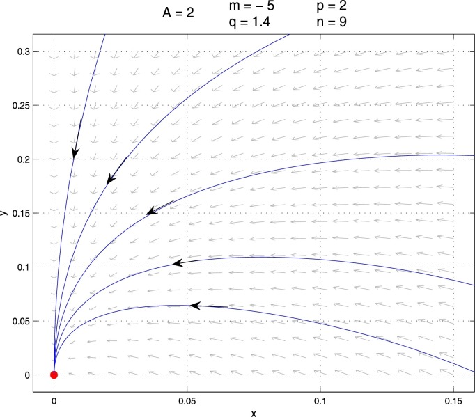
The disease-free equilibrium $E_0(0,0)$ of system (2.3) is a stable hyperbolic node. A phase portrait is shown in Fig. 2.1 .

Fig. 2.1.

The phase portrait of system (2.3) with no positive equilibria for A = 2, m = −5, p = 2, q = 1.4, n = 9.

To discuss whether the disease can invade the population, we study the global stability of the equilibrium $(0,0)$. Since $x=0$ is an invariant line and $\tilde{D}$ is positively invariant, by index theory, we can conclude that system (2.3) does not have nontrivial periodic orbits in ${\mathbb{R}}_{+}^2$ when system (2.3) has no positive equilibria.

Theorem 2.4

The disease-free equilibrium $(\frac{d}{b},0,0)$ of (2.1) is globally asymptotical stable in the interior ${\mathbb{R}}_{+}^3$ and the disease cannot invade the population if $n>n_{⁎}$ , or $n\le n_{⁎}$ and $A\le mp$ .

Remark 2.1

From Theorem 2.4 and system (2.3), we can see that $n>n_{⁎}$ is equivalent to $\alpha >{\alpha }_0$, where

$${\alpha }_0\triangleq \frac{{(bk-\beta d(d+\mu ))}^2(d+\delta )-4k{d}^2(\mu +d)(\mu +d+\delta )}{4d^2(d+\delta ){(\mu +d)}^2},$$ (2.8)

while $n\le n_{⁎}$ and $A\le mp$ are equivalent to $\alpha \le {\alpha }_0$ and $k\le k_0$, where

$$k_0\triangleq \frac{\beta d}{b}(d+\mu ).$$ (2.9)

These indicate that the disease will die out for all positive initial populations when the psychological or inhibitory effect α is greater than a critical value ${\alpha }_0$, or the psychological effect α is smaller than the critical value ${\alpha }_0$ and the infection rate k is also smaller than a critical value $k_0$.

Now we consider the positive equilibria of system (2.3). The positive equilibria with coordinates $(x,y)$ satisfy

$$y=qx,x(A-x-y)-p(1+mx+n{x}^2)=0,$$

and the Jacobian matrix of system (2.3) at a positive equilibrium $E(x,y)$ is given by

$$J(E)=\left[\begin{array}{cc}\hfill \frac{-x^2-px(m+2nx)+x(A-x-qx)}{1+mx+n{x}^2}\hfill & \hfill \frac{-x^2}{1+mx+n{x}^2}\hfill \\ \hfill q\hfill & \hfill -1\hfill \end{array}\right].$$

Then the determinant of $J(E)$ is

$$\det (J(E))=\frac{x[2(np+q+1)x+(mp-A)]}{1+mx+n{x}^2}$$

and its sign is determined by

$$S_D=2(np+q+1)x+(mp-A).$$ (2.10)

The trace of $J(E)$ is

$$\text{tr}(J(E))=\frac{-(2np+n+q+2)x^2+(A-mp-m)x-1}{1+mx+n{x}^2}$$

and its sign is determined by

$$S_T=-(2np+n+q+2)x^2+(A-mp-m)x-1.$$ (2.11)

To discuss the topological type of the positive equilibria of system (2.3), we let

$$q_1=\frac{A^2-2p-Amp}{2p(1+p)},$$ (2.12)

which will be used in the following theorem.

Theorem 2.5

When $n=n_{⁎}$ , $A>mp$ and conditions (2.4) are satisfied, system (2.3) has a unique positive equilibrium $E_{⁎}(x_{⁎},y_{⁎})$ . Moreover,

• (I) if $q\ne q_1$ , then $E_{⁎}(x_{⁎},y_{⁎})$ is a saddle-node, which is attracting (or repelling) if $q<q_1$ (or $q>q_1$ );
• (II) if $q=q_1$ , then $E_{⁎}(x_{⁎},y_{⁎})$ is a cusp of codimension two.

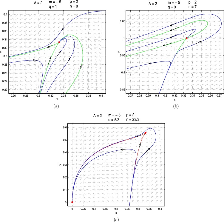
The phase portraits are shown in Fig. 2.2 .

Fig. 2.2.

The phase portraits of system (2.3) with a unique positive equilibrium: (a) an attracting saddle-node for A = 2, m = −5, p = 2, q = 1, n = 8; (b) a repelling saddle-node for A = 2, m = −5, p = 2, q = 3, n = 7; (c) a cusp of codimension two for $A=2,m=-5,p=2,q=\frac{5}{3},n=\frac{23}{3}$.

Proof

Substituting $x_{⁎}$ and $n_{⁎}$ into $S_D$ and $S_T$, we deduce that $S_D(x_{⁎})=0$ and

$$S_T(x_{⁎})=\frac{2[-A^2+Amp+2p+2p(1+p)q]}{{(A-mp)}^2}.$$

Letting $S_T(x_{⁎})=0$, we have

$$q=\frac{A^2-2p-Amp}{2p(1+p)}.$$

Then, using Theorem 7.1 in Zhang et al. [33], we obtain the conclusion in (I).

To show that the assertion (II) holds, let $X=x-x_{⁎}$, $Y=y-y_{⁎}$, $n=n_{⁎}$ and $q=q_1$. Then using Taylor expansions, we can rewrite system (2.3) as follows (for simplicity, we still denote X, Y by x, y, respectively)

$$\begin{array}{cc}\hfill & \frac{dx}{dt}=a_{1}x+a_{2}y+a_3{x}^2+a_{4}xy+o(|(x,y){|}^2),\hfill \\ \hfill & \frac{dy}{dt}=q_{1}x-y,\hfill \end{array}$$ (2.13)

where

$$a_1=1,a_2=-\frac{1}{q_1},a_3=-\frac{{(A-mp)}^2((A-mp)p-2A)}{8p^3{q}_1},a_4=-\frac{A{(A-mp)}^2}{4p^3{q}_1^2}.$$

Next let $X=x$, $Y=x-\frac{1}{q_1}y$. Then system (2.13) is transformed into (we still denote X, Y by x, y, respectively)

$$\begin{array}{cc}\hfill & \frac{dx}{dt}=y+(a_3+q_1{a}_4)x^2-q_1{a}_{4}xy+o(|(x,y){|}^2),\hfill \\ \hfill & \frac{dy}{dt}=(a_3+q_1{a}_4)x^2-q_1{a}_{4}xy+o(|(x,y){|}^2).\hfill \end{array}$$ (2.14)

By Remark 1 of section 2.13 in [24] (see also [15]), we obtain an equivalent system of (2.14) in the small neighborhood of $(0,0)$ as follows:

$$\begin{array}{cc}\hfill & \frac{dx}{d\tau }=y,\hfill \\ \hfill & \frac{dy}{d\tau }=(a_3+q_1{a}_4)x^2+(2a_3+q_1{a}_4)xy+o(|(x,y){|}^2),\hfill \end{array}$$ (2.15)

where

$$a_3+q_1{a}_4=-\frac{{(A-mp)}^3}{8p^2{q}_1},2a_3+q_1{a}_4=-\frac{{(A-mp)}^2((A-mp)p-A)}{4p^3{q}_1}.$$

It is seen that $a_3+q_1{a}_4<0$ because $A>mp$. We next prove $2a_3+q_1{a}_4\ne 0$ (i.e., $m\ne \frac{A(p-1)}{p^2}$) by contradiction. Supposing $m=\frac{A(p-1)}{p^2}$ and substituting it into $n=n_{⁎}$ and $q=q_1$, we obtain

$$n=-\frac{4p^4+A^2(p-1)}{4p^4(1+p)},q=\frac{A^2-2p^2}{2p^2(1+p)}.$$ (2.16)

Further, since $n>0$, $p>q>0$ and $m>-2\sqrt{n}$, it follows from (2.16) that

$$0<p<1,\frac{4p^2}{1-p}<A^2<2p^2(1+p+p^2).$$

However, $\frac{4p^2}{1-p}>2p^2(1+p+p^2)$ if $0<p<1$, which results in a contradiction. Thus $m\ne \frac{A(p-1)}{p^2}$ (i.e., $2a_3+q{a}_4\ne 0$). By the results in [15], $E_{⁎}(x_{⁎},y_{⁎})$ is a cusp of codimension two. □

Remark 2.2

When $m=0$ (i.e., $\beta =0$), our system (2.2) is reduced to system (1.3) in [27], our Theorem 2.5 (II) indicates that Bogdanov-Takens bifurcation of codimension higher than two cannot occur around $E_{⁎}$, which clarifies and corrects the corresponding results in [27], where the authors claimed the existence of Bogdanov-Takens bifurcation of codimension three.

Remark 2.3

When the psychological effect α equals the critical value ${\alpha }_0$ given by (2.8), Theorem 2.5 implies that whether the disease persists or dies out will depend on the infection rate and the initial population. More precisely, when the psychological effect α equals the critical value ${\alpha }_0$ and the infection rate k is greater than the first critical value $k_0$ given by (2.9), i.e., $n=n_{⁎}$ and $A>mp$, then system (2.1) has two equilibria, a disease-free equilibrium and an endemic equilibrium. Moreover, from Fig. 2.2 (b) and (c), we can see that the disease will die out for almost all positive initial populations if the infection rate k is less than another larger critical value

$$k_1\triangleq \frac{\beta d}{b}(d+\mu )+\frac{2d^2(d+\mu )({(d+\delta )}^2+\mu (\mu +\delta +2d))}{b^2{(d+\delta )}^2}(k\le k_1,\text{ i.e.}q\ge q_1),$$ (2.17)

and the disease will persist to a positive coexistent steady state for some positive initial population if the infection rate k is greater than the second critical value $k_1$ ($k>k_1$, i.e. $q<q_1$), as shown in Fig. 2.2 (a).

Theorem 2.6

When $n<n_{⁎}$ , $A>mp$ and conditions (2.4) are satisfied, then system (2.3) has two positive equilibria $E_1(x_1,y_1)$ and $E_2(x_2,y_2)$ . Moreover, $E_1$ is always a hyperbolic saddle and $E_2$ is

• (i) a stable hyperbolic focus (or node) if $S_T(x_2)<0$ ; or
• (ii) a weak focus (or a center) if $S_T(x_2)=0$ ; or
• (iii) an unstable hyperbolic focus (or node) if $S_T(x_2)>0$ ,

where $S_T$ is given in (2.11) .

Proof

To determine the types of $E_1$ and $E_2$, it is suffice to consider the signs of $S_D(x_1)$, $S_D(x_2)$ and $S_T(x_2)$, where $S_D$ and $S_T$ are given in (2.10) and (2.11), respectively, from which we have

$$S_D(x_1)=2(np+q+1)x_1+(mp-A),$$

$$S_D(x_2)=2(np+q+1)x_2+(mp-A).$$

On the other hand, since $x_1$ and $x_2$ are two different positive roots of (2.6), we have

$$(np+q+1)x_1^2+(mp-A)x_1+p=0,2(np+q+1)x_1+(mp-A)<0,$$ (2.18)

$$(np+q+1)x_2^2+(mp-A)x_2+p=0,2(np+q+1)x_2+(mp-A)>0,$$ (2.19)

yielding $S_D(x_1)<0$ and $S_D(x_2)>0$. Hence we obtain the types of $E_1$ and $E_2$. □

Remark 2.4

It is seen from Theorem 2.6 that when the psychological effect α is smaller than the critical value ${\alpha }_0$ but the infection rate k is greater than the first critical value $k_0$, i.e., $n<n_{⁎}$ and $A>mp$, then the disease will become more severe because of the existence of multiple positive coexistent steady states.

3. Bifurcation analysis

From Theorem 2.2, Theorem 2.5, Theorem 2.6, we know that system (2.3) may exhibit saddle-node bifurcation, Bogdanov-Takens bifurcation around the equilibrium $E_{⁎}(x_{⁎},y_{⁎})$, and Hopf bifurcation around the equilibrium $E_2(x_2,y_2)$. In this section, we investigate various possible bifurcations in system (2.3).

3.1. Saddle-node bifurcation

From Theorem 2.2, Theorem 2.5, Theorem 2.6, we know that the surface

$$\mathrm{SN}=\{(A,m,n,p,q):n=n_{⁎},q\ne q_1,-2\sqrt{n}<m<\frac{A}{p},p>q,A,n,p,q>0\}$$

is the saddle-node bifurcation surface. When the parameters are varied to cross the surface from one side to the other side, the number of positive equilibria of system (2.3) changes from zero to two, the saddle-node bifurcation yields two positive equilibria. This implies that there exists a critical psychological effect value ${\alpha }_0$ such that the disease cannot invade the population when $\alpha >{\alpha }_0$ (i.e., $n>n_{⁎}$), and the disease will persist for some positive initial populations when $\alpha \le {\alpha }_0$ (i.e., $n\le n_{⁎}$).

3.2. Bogdanov-Takens bifurcation

In this subsection, we discuss if system (2.3) undergoes Bogdanov-Takens Bifurcation of codimension two under a small parameter perturbation if the bifurcation parameters are chosen suitably. Actually, we have the following theorem.

Theorem 3.1

When $n=n_{⁎}$ , $q=q_1$ , $A>mp$ and conditions (2.4) hold, system (2.3) has a cusp $E_{⁎}(x_{⁎},y_{⁎})$ of codimension two (i.e., Bogdanov-Takens singularity). If we choose A and q as bifurcation parameters, then (2.3) undergoes Bogdanov-Takens bifurcation of codimension two in a small neighborhood of the unique positive equilibrium $E_{⁎}(x_{⁎},y_{⁎})$ . Hence, there exist some parameter values such that system (2.3) has an unstable limit cycle, and there exist some other parameter values such that system (2.3) has an unstable homoclinic loop.

Proof

Consider

$$\begin{array}{cc}\hfill & \frac{dx}{dt}=\frac{x^2}{1+mx+n_{⁎}{x}^2}(A+{\lambda }_1-x-y)-px,\hfill \\ \hfill & \frac{dy}{dt}=(q_1+{\lambda }_2)x-y,\hfill \end{array}$$ (3.1)

where ${\lambda }_1$ and ${\lambda }_2$ are parameters in a small neighborhood of $(0,0)$. We are interested only in the phase portraits of system (3.1) when x and y lie in a small neighborhood of the interior equilibrium $E_{⁎}(x_{⁎},y_{⁎})$.

Let $X=x-x_{⁎}$, $Y=y-y_{⁎}$. Then system (3.1) can be rewritten as (for simplicity, we still denote X, Y by x, y, respectively)

$$\begin{array}{cc}\hfill \frac{dx}{dt}& =b_1+b_{2}x-\frac{1}{q_1}y+b_3{x}^2+b_{4}xy+P_1(x,y,{\lambda }_1,{\lambda }_2),\hfill \\ \hfill \frac{dy}{dt}& =b_5+b_{6}x-y,\hfill \end{array}$$ (3.2)

where $P_1(x,y,{\lambda }_1,{\lambda }_2)$ is a $C^{\infty }$ function at least of third order with respect to $(x,y)$, whose coefficients depend smoothly on ${\lambda }_1$ and ${\lambda }_2$, and

$$\begin{array}{cc}\hfill & b_1={\lambda }_1\frac{1}{q_1},b_2=1+{\lambda }_1\frac{A{(A-mp)}^2}{4p^3{q}_1^2},\hfill \\ \hfill & b_3=-\frac{{(A-mp)}^2}{32p^6{q}_1^3}\left\{4p^3{q}_1^2\right[(A-mp)p-2A]+{\lambda }_1(A-mp)[A^3-A(2Am+6(1+q_1))p\hfill \\ \hfill & +m(Am+2(1+q_1))p^2\left]\right\},\hfill \\ \hfill & b_4=-\frac{A{(A-mp)}^2}{4p^3{q}_1^2},b_5={\lambda }_2\frac{2p}{A-mp},b_6=q_1+{\lambda }_2.\hfill \end{array}$$

Let

$$\begin{array}{cc}\hfill X& =x,\hfill \\ \hfill Y& =b_1+b_{2}x-\frac{1}{q_1}y+b_3{x}^2+b_{4}xy+P_1(x,y,{\lambda }_1,{\lambda }_2),\hfill \end{array}$$

and rewrite X, Y as x, y, respectively. Then system (3.2) becomes

$$\begin{array}{cc}\hfill \frac{dx}{dt}& =y,\hfill \\ \hfill \frac{dy}{dt}& =c_1+c_{2}x+c_{3}y+c_4{x}^2+c_{5}xy+c_6{y}^2+Q_1(x,y,{\lambda }_1,{\lambda }_2),\hfill \end{array}$$ (3.3)

where $Q_1(x,y,{\lambda }_1,{\lambda }_2)$ is a $C^{\infty }$ function at least of third order with respect to $(x,y)$, whose coefficients depend smoothly on ${\lambda }_1$ and ${\lambda }_2$, and

$$\begin{array}{cc}\hfill & c_1=\frac{q_1{b}_1-b_5}{q_1},c_2=\frac{q_1{b}_2+q_1{b}_4{b}_5+q_1^3{b}_1^2{b}_4^2-b_6}{q_1},c_3=0,\hfill \\ \hfill & c_4=b_3+b_4{b}_6+q_1{b}_1{b}_3{b}_4+q_1^2{b}_1{b}_3{b}_4^2,c_5=2b_3+q_1{b}_2{b}_4-q_1^2{b}_1{b}_4^2,c_6=-q_1{b}_4.\hfill \end{array}$$

Next let $dt=(1-c_{6}x)d\tau$, under which system (3.3) becomes (still denote τ by t)

$$\begin{array}{cc}\hfill \frac{dx}{dt}& =y(1-c_{6}x),\hfill \\ \hfill \frac{dy}{dt}& =(1-c_{6}x)(c_1+c_{2}x+c_{3}y+c_4{x}^2+c_{5}xy+c_6{y}^2+Q_1(x,y,{\lambda }_1,{\lambda }_2)).\hfill \end{array}$$ (3.4)

Letting $X=x$, $Y=y(1-c_{6}x)$, and rewriting X, Y as x, y, respectively, we obtain

$$\begin{array}{cc}\hfill \frac{dx}{dt}& =y,\hfill \\ \hfill \frac{dy}{dt}& =d_1+d_{2}x+d_3{x}^2+d_{4}xy+Q_2(x,y,{\lambda }_1,{\lambda }_2),\hfill \end{array}$$ (3.5)

where $Q_2(x,y,{\lambda }_1,{\lambda }_2)$ is a $C^{\infty }$ function at least of third order with respect to $(x,y)$, whose coefficients depend smoothly on ${\lambda }_1$ and ${\lambda }_2$, and

$$d_1=c_1,d_2=c_2-2c_1{c}_6,d_3=c_4-2c_2{c}_6+c_1{c}_6^2,d_4=c_5.$$

Note that when ${\lambda }_1={\lambda }_2=0$,

$$d_1=0,d_2=0,d_3=a_3+q_1{a}_4=-\frac{{(A-mp)}^3}{8p^2{q}_1}<0,$$

$$d_4=2a_3+q_1{a}_4=-\frac{{(A-mp)}^2((A-mp)p-A)}{4p^3{q}_1}<0.$$

Further, let

$$X=x+\frac{d_2}{2d_3},Y=y.$$

Then system (3.5) can be rewritten as (still denote X, Y by x, y, respectively)

$$\begin{array}{cc}\hfill \frac{dx}{dt}& =y,\hfill \\ \hfill \frac{dy}{dt}& =e_1+e_{2}y+e_3{x}^2+e_{4}xy+Q_3(x,y,{\lambda }_1,{\lambda }_2),\hfill \end{array}$$ (3.6)

where $Q_3(x,y,{\lambda }_1,{\lambda }_2)$ is a $C^{\infty }$ function at least of third order with respect to $(x,y)$, whose coefficients depend smoothly on ${\lambda }_1$ and ${\lambda }_2$, and

$$e_1=d_1-\frac{d_2^2}{4d_3},e_2=-\frac{d_2{d}_4}{2d_3},e_3=d_3,e_4=d_4.$$

Making the final change of variables by setting

$$X=\frac{e_4^2}{e_3}x,Y=\frac{e_4^3}{e_3^2}y,\tau =\frac{e_3}{e_4}t,$$

then we finally obtain (still denote X, Y and τ by x, y and t, respectively)

$$\begin{array}{cc}\hfill \frac{dx}{dt}& =y,\hfill \\ \hfill \frac{dy}{dt}& ={\mu }_1+{\mu }_{2}y+x^2+xy+Q_4(x,y,{\lambda }_1,{\lambda }_2),\hfill \end{array}$$ (3.7)

where $Q_4(x,y,{\lambda }_1,{\lambda }_2)$ is a $C^{\infty }$ function at least of third order with respect to $(x,y)$, whose coefficients depend smoothly on ${\lambda }_1$ and ${\lambda }_2$, and

$${\mu }_1=\frac{e_1{e}_4^4}{e_3^3},{\mu }_2=\frac{e_2{e}_4}{e_3}.$$

We can express ${\mu }_1$ and ${\mu }_2$ in terms of ${\lambda }_1$ and ${\lambda }_2$ as follows:

$$\begin{array}{cc}\hfill {\mu }_1& =s_1{\lambda }_1+s_2{\lambda }_2+s_3{\lambda }_1^2+s_4{\lambda }_1{\lambda }_2+s_5{\lambda }_2^2+o(|({\lambda }_1,{\lambda }_2)|),\hfill \\ \hfill {\mu }_2& =t_1{\lambda }_1+t_2{\lambda }_2+t_3{\lambda }_1^2+t_4{\lambda }_1{\lambda }_2+t_5{\lambda }_2^2+o(|({\lambda }_1,{\lambda }_2|),\hfill \end{array}$$ (3.8)

where

$$\begin{array}{cc}\hfill & s_1=-\frac{2{(A-Ap+m{p}^2)}^4}{p^6(A-mp)q_1^2},s_2=\frac{4{(A-Ap+m{p}^2)}^4}{p^5{(A-mp)}^2{q}_1^2},\hfill \\ \hfill & s_3=-\frac{{(A-Ap+m{p}^2)}^3}{4p^{10}(A-mp)q_1^4}\{4m^2{p}^4(1+q_1)+2Am{p}^2[m^2{p}^2+3m^2{p}^3-8p(1+q_1)-6(1+q_1)]\hfill \\ \hfill & +A^{2}p[-5m^2{p}^2-18m^2{p}^3+6p(2-m^2+2q_1)+36(1+q_1)]\hfill \\ \hfill & +A^{3}mp(23+4p+18p^2)-A^4(17+p+6p^2)\},\hfill \\ \hfill & s_4=\frac{{(A-Ap+m{p}^2)}^3}{p^9{(A-mp)}^2{q}_1^4}\{2m^2{p}^4(1+q_1)+Am{p}^2[3m^2{p}^3+p^2(m^2-14q_1)-8p(1+q_1)-6(1+q_1)]\hfill \\ \hfill & +A^{2}p[-9m^2{p}^3+p^2(3m^2+14q_1)+p(6-3m^2-8q_1)+18(1+q_1)]\hfill \\ \hfill & +A^{3}mp(17-9p+9p^2)+A^4(-14+5p-3p^2)\},\hfill \\ \hfill & s_5=-\frac{{(A-Ap+m{p}^2)}^4}{p^8{(A-mp)}^4{q}_1^4}[-11A^4+22A^{3}mp-A^2{p}^2(11m^2+28q_1)+28Am{p}^2+4p^4{q}_1^2],\hfill \\ \hfill & t_1=\frac{A{[A(-1+p)-m{p}^2]}^2}{2p^5{q}_1^2},t_2=\frac{{(A-Ap+m{p}^2)}^2(-A^2+Amp+2p^2{q}_1)}{p^4{(A-mp)}^2{q}_1^2},\hfill \\ \hfill & t_3=\frac{A^2}{4p^9{q}_1^4}[A(-1+p)-m{p}^2]\{A^{2}mp(-8+2p-3p^2)+A^3(6-p+p^2)+m{p}^2[4(1+q_1)\hfill \\ \hfill & -m^2{p}^3]+Ap[m^{2}p(2-p+3p^2)-12(1+q_1)]\},\hfill \\ \hfill & t_4=-\frac{A[A(-1+p)-m{p}^2]}{2p^8{(A-mp)}^2{q}_1^4}\{A^{4}mp(-11+9p-4p^2)+A^5(5-3p+p^2)\hfill \\ \hfill & +A^{2}m{p}^2[8-m^{2}p(1-3p+4p^2)+(8+4p+4p^2+6p^3)q_1]+2m{p}^4{q}_1[m^2{p}^3-2(1+q_1)]\hfill \\ \hfill & +A^{3}p[m^{2}p(7-9p+6p^2)-2(3+(3+p+p^2+p^3)q_1)]+A{p}^3[m^4{p}^3+12q_1(1+q_1)\hfill \\ \hfill & -2m^2(1+(1+p+p^2+3p^3)q_1)]\},\hfill \\ \hfill & t_5=\frac{4A{(A-Ap+m{p}^2)}^2(A^2-Amp+2p^2{q}_1)(-A^2+Amp+2p^2{q}_1)}{p^7{(A-mp)}^3{q}_1^4}.\hfill \end{array}$$

Since

$${\left|\frac{\partial ({\mu }_1,{\mu }_2)}{\partial ({\lambda }_1,{\lambda }_2)}\right|}_{\lambda =0}=-\frac{4{(A-Ap+m{p}^2)}^6}{p^8{(A-mp)}^3{q}_1^3}\ne 0$$

for $m\ne \frac{A(p-1)}{p^2}$, $p>0$, $q_1>0$ and $A>mp$, the parameter transformation (3.8) is a homeomorphism in a small neighborhood of the origin, and ${\mu }_1$ and ${\mu }_2$ are independent parameters.

The results in Bogdanov [3], [4] and Takens [26] now imply that system (3.7) (i.e., (3.1) or (2.3)) undergoes Bogdanov-Takens bifurcation when $({\lambda }_1,{\lambda }_2)$ changes in a small neighborhood of $(0,0)$. □

By the results of Perko [24], we obtain the following local representations of the bifurcation curves up to second-order approximations:

(i) The saddle-node bifurcation curve is

$$\begin{array}{cc}\hfill & \mathrm{SN}=\{({\mu }_1,{\mu }_2)|{\mu }_1=0,{\mu }_2\ne 0\}\hfill \\ \hfill & =\{({\lambda }_1,{\lambda }_2)|-\frac{2{(A-Ap+m{p}^2)}^4}{p^6(A-mp)q_1^2}{\lambda }_1+\frac{4{(A-Ap+m{p}^2)}^4}{p^5{(A-mp)}^2{q}_1^2}{\lambda }_2\hfill \\ \hfill & -\frac{{(A-Ap+m{p}^2)}^3}{4p^{10}(A-mp)q_1^4}\{4m^2{p}^4(1+q_1)+2Am{p}^2[m^2{p}^2+3m^2{p}^3-8p(1+q_1)-6(1+q_1)]+A^{2}p[-5m^2{p}^2\hfill \\ \hfill & -18m^2{p}^3+6p(2-m^2+2q_1)+36(1+q_1)]+A^{3}mp(23+4p+18p^2)-A^4(17+p+6p^2)\}{\lambda }_1^2\hfill \\ \hfill & +\frac{{(A-Ap+m{p}^2)}^3}{p^9{(A-mp)}^2{q}_1^4}\{2m^2{p}^4(1+q_1)+Am{p}^2[3m^2{p}^3+p^2(m^2-14q_1)-8p(1+q_1)-6(1+q_1)]\hfill \\ \hfill & +A^{2}p[-9m^2{p}^3+p^2(3m^2+14q_1)+p(6-3m^2-8q_1)+18(1+q_1)]\hfill \\ \hfill & +A^{3}mp(17-9p+9p^2)+A^4(-14+5p-3p^2)\}{\lambda }_1{\lambda }_2\hfill \\ \hfill & -\frac{{(A-Ap+m{p}^2)}^4}{p^8{(A-mp)}^4{q}_1^4}[-11A^4+22A^{3}mp-A^2{p}^2(11m^2+28q_1)+28Am{p}^2+4p^4{q}_1^2]{\lambda }_2^2=0,{\mu }_2\ne 0\}.\hfill \end{array}$$

(ii) The Hopf bifurcation curve is

$$\begin{array}{cc}\hfill & \mathrm{H}=\{({\mu }_1,{\mu }_2)|{\mu }_2=\sqrt{-{\mu }_1},{\mu }_1<0\}\hfill \\ \hfill & =\{({\lambda }_1,{\lambda }_2)|-\frac{2{(A-Ap+m{p}^2)}^4}{p^6(A-mp)q_1^2}{\lambda }_1+\frac{4{(A-Ap+m{p}^2)}^4}{p^5{(A-mp)}^2{q}_1^2}{\lambda }_2\hfill \\ \hfill & -\frac{{(A-Ap+m{p}^2)}^3}{2p^{10}(A-mp)q_1^4}\{2m^2{p}^4(1+q_1)+Am{p}^2[m^2{p}^2+3m^2{p}^3-8p(1+q_1)-6(1+q_1)]+A^{2}p[-2m^2{p}^2\hfill \\ \hfill & -9m^2{p}^3+p(6-3m^2+6q_1)+18(1+q_1)]+A^{3}mp(12+p+9p^2)-3A^4(3+p^2)\}{\lambda }_1^2\hfill \\ \hfill & +\frac{{(A-Ap+m{p}^2)}^3}{p^9{(A-mp)}^2{q}_1^4}\{2m^2{p}^4(1+q_1)+Am{p}^2[3m^2{p}^3+p^2(m^2-12q_1)-8p(1+q_1)-6(1+q_1)]\hfill \\ \hfill & +A^{2}p[-9m^2{p}^3+4p^2(m^2+3q_1)-3p(-2+m^2+2q_1)+18(1+q_1)]\hfill \\ \hfill & +A^{3}mp(18-11p+9p^2)-3A^4(5-2p+p^2)\}{\lambda }_1{\lambda }_2\hfill \\ \hfill & +\frac{12A{(A-Ap+m{p}^2)}^4(A^2-Amp+2p^{2}q)}{p^8{(A-mp)}^3{q}_1^4}{\lambda }_2^2=0,{\mu }_1<0\}.\hfill \end{array}$$

(iii) The homoclinic bifurcation curve is

$$\begin{array}{cc}\hfill & \mathrm{HL}=\{({\mu }_1,{\mu }_2)|{\mu }_2=\frac{5}{7}\sqrt{-{\mu }_1},{\mu }_1<0\}\hfill \\ \hfill & =\{({\lambda }_1,{\lambda }_2)|-\frac{50{(A-Ap+m{p}^2)}^4}{49p^6(A-mp)q_1^2}{\lambda }_1+\frac{100{(A-Ap+m{p}^2)}^4}{49p^5{(A-mp)}^2{q}_1^2}{\lambda }_2\hfill \\ \hfill & -\frac{{(A-Ap+m{p}^2)}^3}{98p^{10}(A-mp)q_1^4}\{50m^2{p}^4(1+q_1)+25Am{p}^2[m^2{p}^2+3m^2{p}^3-8p(1+q_1)-6(1+q_1)]\hfill \\ \hfill & +A^{2}p[-38m^2{p}^2-225m^2{p}^3-75p(-2+m^2-2q_1)+450(1+q_1)]\hfill \\ \hfill & +A^{3}mp(312+p+225p^2)-3A^4(79-4p+25p^2)\}{\lambda }_1^2\hfill \\ \hfill & +\frac{{(A-Ap+m{p}^2)}^3}{49p^9{(A-mp)}^2{q}_1^4}\{50m^2{p}^4(1+q_1)+Am{p}^2[75m^2{p}^3+p^2(25m^2-252q_1)-200p(1+q_1)\hfill \\ \hfill & -150(1+q_1)]+A^{2}p[-225m^2{p}^3+4p^2(31m^2+63q_1)-3p(-50+25m^2+34q_1)+450(1+q_1)]\hfill \\ \hfill & +A^{3}mp(474-323p+225p^2)-3A^4(133-58p+25p^2)\}{\lambda }_1{\lambda }_2\hfill \\ \hfill & +\frac{12{(A-Ap+m{p}^2)}^4}{49p^8{(A-mp)}^3{q}_1^4}[27A^4-54A^{3}mp-42Am{p}^3+8p^4{q}_1^2+3A^2{p}^2(9m^2+16q_1)]{\lambda }_2^2=0,{\mu }_1<0\}.\hfill \end{array}$$

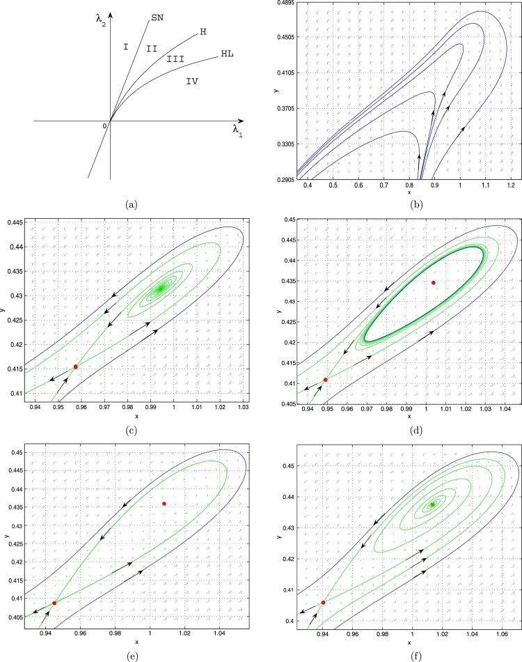
The Bogdanov-Takens bifurcation diagram and corresponding phase portraits of system (3.1) are given in Fig. 3.1 , where we fix $A=2$, $m=-1$, $p=2$, $q=1/3$ and $n=1/3$, which satisfy $n=n_{⁎}$, $q=q_1$, $A>mp$ and conditions (2.4), and then perturb A and q. The bifurcation curves $\mathrm{H},\mathrm{HL}$ and SN divide the small neighborhood of the origin in the parameter $({\lambda }_1,{\lambda }_2)$-plane into four regions (see Fig. 3.1(a)).

Fig. 3.1.

The bifurcation diagram and phase portraits of system (3.1) for A = 2, m = −1, p = 2, q = 1/3, n = 1/3. (a) Bifurcation diagram; (b) No positive equilibria when (λ₁,λ₂)=(0.1,0.11) lies in the region I; (c) An unstable focus when (λ₁,λ₂)=(0.1,0.1005) lies in the region II; (d) An unstable limit cycle when (λ₁,λ₂)=(0.1,0.0996) lies in the region III; (e) An unstable homoclinic loop when (λ₁,λ₂)=(0.1,0.09905427) lies on the curve HL; (f) A stable focus when (λ₁,λ₂)=(0.1,0.0983) lies in the region IV.

(a) When $({\lambda }_1,{\lambda }_2)=(0,0)$, the unique positive equilibrium is a cusp of codimension two (see Fig. 2.2(c)).

(b) There are no equilibria when the parameters lie in region I (see Fig. 3.1(b)), implying that the disease dies out.

(c) When the parameters lie on the curve SN, there is a unique positive equilibrium $E_{⁎}$, which is a saddle-node.

(d) Two positive equilibria, one is an unstable focus $E_2$ and the other is a saddle $E_1$, will occur through the saddle-node bifurcation when the parameters cross the SN curve into region II (see Fig. 3.1(c)).

(e) An unstable limit cycle will appear through the subcritical Hopf bifurcation around $E_2$ when the parameters are varied to cross the H curve into region III (see Fig. 3.1(d)), where the focus $E_2$ is stable, whereas the focus $E_2$ is an unstable one with multiplicity one when the parameters lie on the curve H.

(f) An unstable homoclinic orbit will occur through the homoclinic bifurcation around $E_1$ when the parameters pass region III and lie on the curve HL (see Fig. 3.1(e)).

(g) The relative location of one stable and one unstable manifold of the saddle $E_1$ will be reversed when the parameters are varied to cross the HL curve into region IV (compare Fig. 3.1(c) and Fig. 3.1(f)).

3.3. Hopf bifurcation

In this subsection we discuss Hopf bifurcation around the equilibrium $E_2(x_2,y_2)$. Let

$$\begin{array}{cc}\hfill & a_{⁎}=\frac{p-1-np}{n+m+1},q_2=-\frac{c_0+c_{1}m+c_2{m}^2}{d_0+d_{1}m+d_2{m}^2},m_1=\frac{{(p-1-np)}^2-p(n+1)}{p},m_2=-2\sqrt{n},\hfill \\ \hfill & m_3=\frac{-n(1+(3+n)p)-\sqrt{n^2{(1+(3+n)p)}^2-4p(3n-1)(1+2np)}}{2p},\hfill \\ \hfill & m_4=\frac{-n(1+(3+n)p)+\sqrt{n^2{(1+(3+n)p)}^2-4p(3n-1)(1+2np)}}{2p},\hfill \\ \hfill & c_0=3n-1+(3-4n+9n^2)p+2n(3-2n+3n^2)p^2,c_1=n+(3+3n+2n^2)p+{(n+1)}^3{p}^2,\hfill \\ \hfill & c_2=2p(1+np),d_0=(3n-1)(1+2np),d_1=n(1+(3+n)p),d_2=p,\hfill \\ \hfill & p_{⁎}=\frac{3-2\sqrt{n}-n+\sqrt{5-12n^{1/2}+6n+4n^{3/2}-3n^2}}{2{(n-1)}^2},\hfill \end{array}$$ (3.9)

which will be used in the following subsection.

To simplify the computation, by following the technique in [11], we reduce system (2.3) to an equivalent polynomial differential system by using the following state variable scaling and time rescaling:

$$\bar{x}=\frac{x}{x_2},\bar{y}=\frac{y}{y_2},\tau =x_2^{2}t,$$ (3.10)

under which system (2.3) is transformed into (we still denote τ by t)

$$\begin{array}{cc}\hfill \frac{d\bar{x}}{dt}& =\frac{{\bar{x}}^2}{1+m{x}_2\bar{x}+n{x}_2^2{\bar{x}}^2}(\frac{A}{x_2}-\bar{x}-q\bar{y})-\frac{p}{x_2^2}\bar{x},\hfill \\ \hfill \frac{d\bar{y}}{dt}& =\frac{1}{x_2^2}(\bar{x}-\bar{y}).\hfill \end{array}$$ (3.11)

Then taking the parameter scaling,

$$\bar{A}=\frac{A}{x_2},\bar{m}=m{x}_2,\bar{n}=n{x}_2^2,\bar{p}=\frac{p}{x_2^2},\bar{q}=q,a=\frac{1}{x_2^2},$$

into system (3.11) and dropping the bars, we obtain

$$\begin{array}{cc}\hfill \frac{dx}{dt}& =\frac{x^2}{1+mx+n{x}^2}(A-x-qy)-px,\hfill \\ \hfill \frac{dy}{dt}& =a(x-y).\hfill \end{array}$$ (3.12)

Since system (3.12) has an equilibrium ${\tilde{E}}_2(1,1)$ (i.e., $E_2(x_2,y_2)$ of system (2.3)), we have

$$A=p(1+m+n)+q+1.$$

Note that $x_1{x}_2=\frac{p}{np+q+1}$ for system (2.3), which becomes $\frac{x_1}{x_2}=\frac{\bar{p}}{\bar{n}\bar{p}+\bar{q}+1}$ under the parameter scaling (3.10), dropping the bars, so we have $np+q+1-p>0$ because $\frac{x_1}{x_2}<1$. Regarding the above parameter scaling, the condition (2.4), $n<n_{⁎}$ and $A>mp$ become

$$p,q,n,a>0,p-1-np<q<\frac{p}{a},m>-2\sqrt{n}.$$ (3.13)

Since the transformation (3.10) is a linear sign-reserving transformation, system (3.12) and system (2.3) have the same qualitative property.

Next letting $dt=(1+mx+n{x}^2)d\tau$ and substituting $A=p(1+m+n)+q+1$ into (3.12), we obtain (still denote τ by t)

$$\begin{array}{cc}\hfill \frac{dx}{dt}& =x^2[p(1+m+n)+q+1-x-qy]-p(1+mx+n{x}^2)x,\hfill \\ \hfill \frac{dy}{dt}& =a(x-y)(1+mx+n{x}^2),\hfill \end{array}$$ (3.14)

where m, p, q, n, a satisfy (3.13). Obviously system (3.14) has the same topological structure as that of system (3.12), since we consider system (3.12) in ${\mathbb{R}}_2^{+}=\{(x,y):x\ge 0,y\ge 0\}$, and $1+mx+n{x}^2>0$ holds for all $x\ge 0$. In the following, we study the Hopf bifurcation around ${\tilde{E}}_2(1,1)$ in system (3.14), which corresponds to the Hopf bifurcation around $E_2(x_2,y_2)$ in system (2.3).

Theorem 3.2

When conditions in (3.13) hold, system (3.14) has an equilibrium at ${\tilde{E}}_2(1,1)$ . Moreover,

• (I) when $a<a_{⁎}$ , ${\tilde{E}}_2(1,1)$ is an unstable hyperbolic node or focus;
• (II) when $a>a_{⁎}$ , ${\tilde{E}}_2(1,1)$ is a locally asymptotically stable hyperbolic node or focus;
• (III) when $a=a_{⁎}$ , ${\tilde{E}}_2(1,1)$ is a fine focus or center.

Proof

The Jacobian matrix of system (3.14) at ${\tilde{E}}_2(1,1)$ is

$$J({\tilde{E}}_2(1,1))=\left[\begin{array}{cc}\hfill p-1-np\hfill & \hfill -q\hfill \\ \hfill a(m+n+1)\hfill & \hfill -a(m+n+1)\hfill \end{array}\right].$$

Then the determinant of $J({\tilde{E}}_2(1,1))$ is

$$\det (J({\tilde{E}}_2))=a(m+n+1)(np+q+1-p),$$

and the trace of $J({\tilde{E}}_2(1,1))$ is

$$\text{tr}(J({\tilde{E}}_2))=p-1-np-a(m+n+1).$$

By conditions in (3.13), we can see that $\det (J({\tilde{E}}_2))>0$ and $\text{tr}(J({\tilde{E}}_2))=0$ (>0 or <0) if $a=a_{⁎}$ ($a<a_{⁎}$ or $a>a_{⁎}$), so the conclusions follow. □

Next we continue to consider the case (III) of Theorem 3.1 and study Hopf bifurcation around ${\tilde{E}}_2(1,1)$ in system (3.14). We have the following necessary conditions for Hopf bifurcation:

$$a=a_{⁎},0<n<1,p>\frac{1}{1-n},m>-2\sqrt{n},p-1-np<q<\frac{p}{a_{⁎}}.$$ (3.15)

Firstly we can check the transversality condition

$$\frac{\mathrm{d}}{\mathrm{d}a}(\mathrm{tr}J({\tilde{E}}_2)){|}_{a=a⁎}=-(m+n+1)<0.$$

We investigate the nondegenerate condition and stability of the bifurcating periodic orbit from the positive equilibrium ${\tilde{E}}_2(1,1)$ of system (3.14) by calculating the first Lyapunov coefficient.

Let $X=x-1$, $Y=y-1$, and $a=a_{⁎}$. Then system (3.14) can be written as (still denote X, $Y,\tau$ by x, $y,t$, respectively)

$$\begin{array}{cc}\hfill \frac{dx}{dt}& =\tilde{b}x-qy+(p-2-2np)x^2-2qxy-(1+np)x^3-q{x}^{2}y,\hfill \\ \hfill \frac{dy}{dt}& =\tilde{b}x-\tilde{b}y+a_{⁎}(m+2n)x^2-a_{⁎}(m+2n)xy+a_{⁎}n{x}^3-a_{⁎}n{x}^{2}y,\hfill \end{array}$$ (3.16)

where $\tilde{b}=p-1-np$. Let $\omega =\sqrt{\tilde{b}q-{\tilde{b}}^2}$, and make a transformation of $x=X$, $y=\frac{1}{q}(\tilde{b}X-\omega Y)$ and $dt=\frac{1}{\omega }d\tau$, then system (3.16) becomes (we still denote X, Y by x, y, respectively)

$$\begin{array}{cc}\hfill \frac{dx}{dt}& =y+f(x,y),\hfill \\ \hfill \frac{dy}{dt}& =-x+g(x,y),\hfill \end{array}$$ (3.17)

where

$$f(x,y)=a_{20}{x}^2+a_{11}xy+a_{02}{y}^2+a_{30}{x}^3+a_{21}{x}^{2}y+a_{12}x{y}^2+a_{03}{y}^3,$$

$$g(x,y)=b_{20}{x}^2+b_{11}xy+b_{02}{y}^2+b_{30}{x}^3+b_{21}{x}^{2}y+b_{12}x{y}^2+b_{03}{y}^3,$$

and

$$a_{20}=-\frac{p}{\omega },a_{11}=2,a_{02}=0,a_{30}=-\frac{p}{\omega },a_{21}=1,a_{12}=0,a_{03}=0,$$

$$b_{20}=\frac{1}{{\omega }^2}(-\tilde{b}p+a_{⁎}(m+2n)(\tilde{b}-q)),b_{11}=\frac{1}{\omega }(2\tilde{b}-a_{⁎}(m+2n)),b_{02}=0,$$

$$b_{30}=-\frac{1}{{\omega }^2}(\tilde{b}p+a_{⁎}n(q-\tilde{b})),b_{21}=\frac{\tilde{b}-a_{⁎}n}{\omega },b_{12}=0,b_{03}=0.$$

Using the formula in [33] and calculating first Lyapunov coefficient with the aid of MATLAB, we obtain

$${\sigma }_1=\frac{(c_0+c_{1}m+c_2{m}^2)+(d_0+d_{1}m+d_2{m}^2)q}{4{(1+m+n)}^2{(np+q+1-p)}^{3/2}{(p-1-np)}^{1/2}},$$ (3.18)

where $c_0$, $c_1$, $c_2$, $d_0$, $d_1$ and $d_2$ are given in (3.9). By conditions in (3.15), the sign of ${\sigma }_1$ is the same as that of

$${\sigma }_{11}=(c_0+c_{1}m+c_2{m}^2)+(d_0+d_{1}m+d_2{m}^2)q.$$ (3.19)

Now we investigate the sign of ${\sigma }_{11}$ (i.e., ${\sigma }_1$) and will see that there exist some values of parameters such that ${\sigma }_{11}=0$ (i.e., ${\sigma }_1=0$) when conditions (3.15) are satisfied. We first give the following Lemma.

Lemma 3.3

When conditions (3.15) are satisfied, then $c_0+c_{1}m+c_2{m}^2>0$ , where $c_i$ $(i=0,1,2)$ are given in (3.9) .

Proof

By conditions (3.15), it is easy to show that $c_i>0$ $(i=0,1,2)$ and

$$m>-2\sqrt{n},p-1-np<q<\frac{p}{a_{⁎}}=\frac{p(m+n+1)}{p-1-np}.$$

Then we have

$$m>\max \{m_1,m_2\},$$

where $m_1$ and $m_2$ are given in (3.9).

(I) Firstly, we consider the discriminant of $c_0+c_{1}m+c_2{m}^2=0$, which is given by

$$\mathrm{\Delta }(p)=c_1^2-4c_0{c}_2={\mathrm{\Delta }}_0+{\mathrm{\Delta }}_{1}p+{\mathrm{\Delta }}_2{p}^2+{\mathrm{\Delta }}_3{p}^3+{\mathrm{\Delta }}_4{p}^4,$$

where

$${\mathrm{\Delta }}_0=n^2>0,{\mathrm{\Delta }}_1=8-18n+6n^2+4n^3,{\mathrm{\Delta }}_2=-15+60n-69n^2+18n^3+6n^4,$$

$${\mathrm{\Delta }}_3=6-48n+104n^2-84n^3+18n^4+4n^5,{\mathrm{\Delta }}_4=1+6n-33n^2+52n^3-33n^4+6n^5+n^6.$$

We consider the third derivative of $\mathrm{\Delta }(p)$ with respect to p, which is given by

$${\mathrm{\Delta }}^{(3)}(p)=6{\mathrm{\Delta }}_3+24{\mathrm{\Delta }}_{4}p.$$

Because ${\mathrm{\Delta }}^{(3)}(\frac{1}{1-n})=60{(1-n)}^3(1+n)>0$, we can show that ${\mathrm{\Delta }}_4>0$ when $0<n<1$. Thus

$${\mathrm{\Delta }}^{(3)}(p)>0\mathrm{for}p>\frac{1}{1-n}.$$

On the other hand, we have ${\mathrm{\Delta }}_p^{″}(\frac{1}{1-n})=18{(n-1)}^2>0$, and so

$${\mathrm{\Delta }}_p^{″}(p)>0\mathrm{for}p>\frac{1}{1-n}.$$

Similarly, we have ${\mathrm{\Delta }}_p^{\prime }(\frac{1}{1-n})=0$ and $\mathrm{\Delta }(\frac{1}{1-n})=0$, which yield

$$\mathrm{\Delta }(p)>0\mathrm{for}p>\frac{1}{1-n}.$$

(II) Secondly, we analyze the sign of $m_1-m_2$, which is same as

$$m_{12}(p)=1+(2\sqrt{n}+n-3)p+{(n-1)}^2{p}^2.$$

By noticing $0<n<1$ and using a simple analysis, we have

$$2\sqrt{n}+n-3<0,-\frac{2\sqrt{n}+n-3}{2{(n-1)}^2}-\frac{1}{1-n}=\frac{{(\sqrt{n}-1)}^2}{2(n-1)}>0,m_{12}(\frac{1}{1-n})=\frac{\sqrt{n}-1}{\sqrt{n}+1}<0.$$

Thus, we can see that $m_{12}(p)>0$, $m_{12}(p)=0$ and $m_{12}(p)<0$ if and only if $p>p_{⁎}$, $p=p_{⁎}$ and $\frac{1}{1-n}<p<p_{⁎}$, respectively, where $p_{⁎}=\frac{3-2\sqrt{n}-n+\sqrt{5-12n^{1/2}+6n+4n^{3/2}-3n^2}}{2{(n-1)}^2}$ $(>\frac{1}{1-n})$.

(III) Thirdly, we analyze the relationship between $-\frac{c_1}{2c_2}$ and $m_1$, $m_2$. The sign of $-\frac{c_1}{2c_2}-m_1$ is the same as that of

$$m_{s1}(p)=-4-n+(9-11n-2n^2)p+(-5+17n-11n^2-n^3)p^2-4n{(n-1)}^2{p}^3.$$

The first derivative of $m_{s1}$ with respect to p is

$$m_{s1}^{\prime }(p)=9-11n-2n^2+2(-5+17n-11n^2-n^3)p-12n{(n-1)}^2{p}^2.$$

Since $0<n<1$ and $p>\frac{1}{1-n}$, one can prove that $m_{s1}^{\prime }(p)<0$. Moreover, we have $m_{s1}(\frac{1}{1-n})=0$. Thus we have $m_{s1}(p)<0$, i.e., $m_1>-\frac{c_1}{2c_2}$, when conditions (3.15) are satisfied.

The sign of $-\frac{c_1}{2c_2}-m_2$ is the same as that of

$$m_{s2}(p)=-n+(-3+8n^{1/2}-3n-2n^2)p+(-1-3n+8n^{3/2}-3n^2-n^3)p^2.$$

Since $0<n<1$, by a direct computation, we can show that

$$-1-3n+8n^{3/2}-3n^2-n^3<0,$$

$$-\frac{-3+8n^{1/2}-3n-2n^2}{2(-1-3n+8n^{3/2}-3n^2-n^3)}-\frac{1}{1-n}=\frac{5+2\sqrt{n}+5n}{2(n^2-1)(1+2\sqrt{n}+6n+2n^{3/2}+n^2)}<0,$$

and

$$m_{s2}(\frac{1}{1-n})=\frac{-4}{{(1+\sqrt{n})}^2}<0.$$

It then follows that $m_{s2}(p)<0$, i.e., $m_2>-\frac{c_1}{2c_2}$, when conditions (3.15) are satisfied.

(IV) Finally, we show that $c(m)=c_0+c_{1}m+c_2{m}^2>0$ when conditions (3.15) are satisfied. When $p\ge p_{⁎}$ $(>\frac{1}{1-n})$, we have $m_1\ge m_2$ by the step (II), then $m>\max \{m_1,m_2\}=m_1$ and $c(m)>c(m_1)$ by the step (III). Moreover, we can show that $c(m_1)>0$. In fact, the sign of $c(m_1)$ is the same as that of

$$c_{m1}(p)=2+n+(-6+7n+n^2)p+(3-9n+5n^2+n^3)p^2+2n{(n-1)}^2{p}^3.$$

By a direct computation with conditions in (3.15), we have

$$c_{m1}(\frac{1}{1-n})=n-1<0,c_{m1}(p_{⁎})=\frac{c_{1⁎}}{2(1-\sqrt{n}){(1+\sqrt{n})}^4},$$

where

$$c_{1⁎}=7+(3+3\sqrt{n}+5n+3n^{3/2}+2n^2)\sqrt{{(1-\sqrt{n})}^3(5+3\sqrt{n})}-\sqrt{n}(3+2\sqrt{n}+4n)-n^2(-5+\sqrt{n}+2n).$$

We can see that $c_{1⁎}$ is monotonic decreasing for $0<n<1$. Moreover, since $c_{1⁎}(0)=7$ and $c_{1⁎}(1)=0$, we have $c_{1⁎}>0$ (i.e., $c_{m_1}(p_{⁎})>0$) when $0<n<1$, and thus $c(m_1)(p)>0$, i.e., $c(m_1)>0$, when $p>p_{⁎}$.

When $\frac{1}{1-n}<p<p_{⁎}$, we have $m_1<m_2$ by the step (II), then $m>\max \{m_1,m_2\}=m_2$ and $c(m)>c(m_2)$ by the step (III). Moreover, we can show that $c(m_2)>0$. In fact, the sign of $c(m_2)$ is same as

$$c_{m2}(p)=-1-2\sqrt{n}+(3+n-4n^{3/2})p-2\sqrt{n}{(-1+\sqrt{n})}^2(1+\sqrt{n}+n)p^2.$$

By direct computation, we have $c_{m2}(\frac{1}{1-n})=\frac{2}{{(1+\sqrt{n})}^2}>0$ and $c_{m2}(p_{⁎})=c_{m_1}(p_{⁎})>0$. Then $c(m_2)(p)>0$, i.e., $c(m_2)>0$, when $\frac{1}{1-n}<p<p_{⁎}$.

Summarizing the above results, we have shown that $c_0+c_{1}m+c_2{m}^2>0$ when conditions (3.15) are satisfied. □

Lemma 3.4

When the conditions in (3.15) are satisfied, $d_0+d_{1}m+d_2{m}^2<0$ if and only if $m_3<m<m_4$ , where $d_i$ $(i=0,1,2)$ and $m_j$ $(j=3,4)$ are given in (3.9) .

Proof

Let

$$d(m)=d_0+d_{1}m+d_2{m}^2,$$

where

$$d_0=(3n-1)(1+2np)d_1=n(1+(3+n)p)>0,d_2=p>0.$$

We then show that

$$d_1^2-4d_0{d}_2=n^2+2(n^3+3n^2-6n+2)p+n(n^3+6n^2-15n+8)p^2>0.$$

In fact, let

$$h(p)=n^2+2(n^3+3n^2-6n+2)p+n(n^3+6n^2-15n+8)p^2.$$

By the conditions in (3.15), we obtain

$$n(n^3+6n^2-15n+8)>0,$$

and

$$h(-\frac{n^3+3n^2-6n+2}{n(n^3+6n^2-15n+8)})=\frac{4(1-n)(3n-1)}{n(8+n)}.$$

Then when $\frac{1}{3}<n<1$, we have

$$h(p)>0;$$

when $0<n\le \frac{1}{3}$, we have

$$2(n^3+3n^2-6n+2)>0,$$

and

$$h(0)=n^2>0,$$

thus

$$h(p)>0.$$

From the above analysis, we have $d_1^2-4d_0{d}_2>0$ when conditions (3.15) are satisfied, implying that the equation $d(m)=0$ has two positive roots:

$$m_3=\frac{-n(1+(3+n)p)-\sqrt{n^2{(1+(3+n)p)}^2-4p(3n-1)(1+2np)}}{2p},$$

$$m_4=\frac{-n(1+(3+n)p)+\sqrt{n^2{(1+(3+n)p)}^2-4p(3n-1)(1+2np)}}{2p},$$

and $d(m)<0$ if and only if $m_3<m<m_4$. □

Theorem 3.5

When the conditions in (3.15) are satisfied, the following statements hold.

• (I) If $m\le m_3$ or $m\ge m_4$ (i.e., ${\sigma }_{11}>0$ or ${\sigma }_1>0$ ), then system (3.14) exhibits subcritical Hopf bifurcation and an unstable limit cycle appears around ${\tilde{E}}_2(1,1)$ .
• (II)
  If $m_3<m<m_4$ and

  • (II.1)
    $q>q_2$ (i.e., ${\sigma }_{11}<0$ or ${\sigma }_1<0$ ), then system (3.14) exhibits supercritical Hopf bifurcation and a stable limit cycle appears around ${\tilde{E}}_2(1,1)$ ;
  • (II.2)
    $q<q_2$ (i.e., ${\sigma }_{11}>0$ or ${\sigma }_1>0$ ), then system (3.14) exhibits subcritical Hopf bifurcation and an unstable limit cycle appears around ${\tilde{E}}_2(1,1)$ ;
  • (II.3)
    $q=q_2$ (i.e., ${\sigma }_{11}=0$ or ${\sigma }_1=0$ ), then system (3.14) may exhibits degenerate Hopf bifurcation and multiple limit cycles may appears around ${\tilde{E}}_2(1,1)$ .

Here, $m_3$ , $m_4$ and $q_2$ are given in (3.9) .

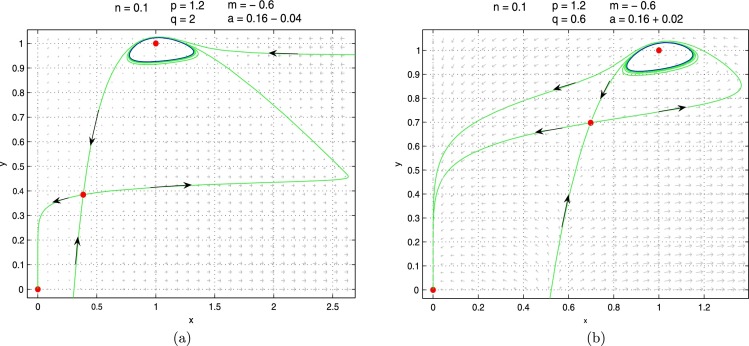
One stable (or unstable) limit cycle arising from supercritical (or subcritical) Hopf bifurcation around the equilibrium ${\tilde{E}}_2(1,1)$ of system (3.14) is given in Fig. 3.2 . In Fig. 3.2(a), we fix $n=0.1$, $p=1.2$, $m=-0.6$ and $q=2$, and get $a=0.16$ from $\text{tr}(J({\tilde{E}}_2))=0$, and further obtain ${\sigma }_1=-3.24949$. Finally, we perturb a such that a decreases to 0.12, then ${\tilde{E}}_2(1,1)$ becomes an unstable hyperbolic focus, leading to a stable limit cycle to appear around ${\tilde{E}}_2(1,1)$. In Fig. 3.2(b), we fix $n=0.1$, $p=1.2$, $m=-0.6$ and $q=0.6$, and get $a=0.16$ from $\text{tr}(J({\tilde{E}}_2))=0$, and further get ${\sigma }_1=2.62886$. Finally, we perturb a such that a increases to 0.18, and so ${\tilde{E}}_2(1,1)$ becomes a stable hyperbolic focus, yielding an unstable limit cycle to appear around ${\tilde{E}}_2(1,1)$.

Fig. 3.2.

(a) A stable limit cycle created by the supercritical Hopf bifurcation of the system (3.14) with n = 0.1, p = 1.2, m = −0.6, q = 2 and a = 0.12. (b) An unstable limit cycle created by the subcritical Hopf bifurcation of the system (3.14) with n = 0.1, p = 1.2, m = −0.6, q = 0.6 and a = 0.18.

Remark 3.1

In Fig. 3.2(a), the model has three equilibria, a disease-free equilibrium which is a stable hyperbolic node, two endemic equilibria (one is a hyperbolic saddle and the other is an unstable focus) and a stable limit cycle. If the initial population lies on the right side of the two stable manifolds of the saddle, then the disease will tend to a periodic coexistent oscillation. If the initial population lies on the left side of the two stable manifolds of the saddle, then the disease will die out.

Remark 3.2

In Fig. 3.2(b), the model has three equilibria, a disease-free equilibrium which is a stable hyperbolic node, two endemic equilibria (one is a hyperbolic saddle and the other is a stable focus) and an unstable limit cycle. If the initial population lies on the limit cycle, then the disease will persist in the form of a periodic coexistent oscillation. If the initial population lies inside the limit cycle, then the disease will tend to a stable steady state. If the initial population lies outside the limit cycle, the disease will die out for almost all positive initial populations.

3.4. Degenerate Hopf bifurcation of codimension two

From (II.3) of Theorem 3.5, we know that system (3.14) may exhibit degenerate Hopf bifurcation (i.e., Hopf bifurcation of codimension two) when $q=q_2$, $m_3<m<m_4$ and conditions (3.15) are satisfied. Using the formal series method in [33] and MATLAB software, we obtain the second Lyapunov coefficient

$${\sigma }_2=\frac{e_0+e_{1}m+e_2{m}^2+e_3{m}^3}{24{(m+n+1)}^3(2+4np+m(np+p+1))\sqrt{\frac{(m+n+1)p(p-1-np)(2+4np+m(np+p+1))}{-(d_0+d_{1}m+d_2{m}^2)}}},$$ (3.20)

where

$$\begin{array}{cc}\hfill e_0& =3(1-n^2){(1+2np)}^2,e_1=n^2-9n+4+(3n^3-31n^2+21n-1)p+2n(n^3-13n^2+13n-1)p^2,\hfill \\ \hfill e_2& =-4n-(3+5n^2)p+n(1-n^2)p^2,e_3=-n-2(n^2-2n+2)p+(1-4n+4n^2-n^3)p^2.\hfill \end{array}$$

Next we investigate the sign of ${\sigma }_2$ and first give the following lemma.

Lemma 3.6

When conditions in (3.15) are satisfied, the inequality $2+4np+m(np+p+1)>0$ holds.

Proof

Let

$$h(m)=2+4np+m(np+p+1).$$

When $p\ge p_{⁎}$ $(>\frac{1}{1-n})$, we have $m_1\ge m_2$ by the step (II) of Lemma 3.3. Then $m>\max \{m_1,m_2\}=m_1$ and $h(m)>h(m_1)$. Moreover, we can show that $h(m_1)>0$. In fact, the sign of $h(m_1)$ is the same as that of

$$h(m_1)(p)=1+2np+2(n^2-1)p^2+{(n-1)}^2(n+1)p^3.$$

By a direct calculation, we have

$$h(m_1){(p)}^{\prime }=2n+4(n^2-1)p+3{(n-1)}^2(n+1)p^2.$$

It follows that $h(m_1){(p)}^{\prime }>0$ when $p>p_{⁎}$. Further, by a direct calculation, we have

$$h(m_1)(p_{⁎})=\frac{3+3n+2n^{3/2}+\sqrt{{(1-\sqrt{n})}^3(5+3\sqrt{n})}}{{(1+\sqrt{n})}^4}>0,$$

so $h(m_1)(p)>0$ (i.e., $h(m_1)>0$) when $p>p_{⁎}$.

When $\frac{1}{1-n}<p<p_{⁎}$, we have $m_1<m_2$ by the step (II) in the proof of Lemma 3.3. Then $m>\max \{m_1,m_2\}=m_2$ and $h(m)>h(m_2)$. Moreover, we can show that $h(m_2)>0$. In fact

$$h(m_2)=2(1-\sqrt{n})[1-\sqrt{n}(1-\sqrt{n})p].$$

By a direct calculation, we have

$$h(m_2)\left(\frac{1}{1-n}\right)=\frac{2(1-\sqrt{n})}{1+\sqrt{n}},$$

$$h(m_2)(p_{⁎})=\frac{2-\sqrt{n}-n^{3/2}-\sqrt{n}\sqrt{{(1-\sqrt{n})}^3(5+3\sqrt{n})}}{{(1+\sqrt{n})}^2}.$$

It follows that $h(m_2)(\frac{1}{1-n})>0$ and $h(m_2)(p_{⁎})>0$ for $0<n<1$. Thus, $h(m_2)>0$ when $\frac{1}{1-n}<p<p_{⁎}$.

Summarizing the above results, we have shown that $h(m)>0$ (i.e., $2+4np+m(np+p+1)>0$) when conditions (3.15) are satisfied. □

When $m>-2\sqrt{n}$, $0<n<1$, $p>\frac{1}{1-n}$, $m_3<m<m_4$, and by Lemma 3.6, we know that the sign of ${\sigma }_2$ in (3.20) is the same as that of

$$e_0+e_{1}m+e_2{m}^2+e_3{m}^3\triangleq {\sigma }_{21}.$$ (3.21)

Based on extensive numerical calculations, we conjecture that ${\tilde{E}}_2(1,1)$ is an unstable multiple focus with multiplicity two, i.e., ${\sigma }_{21}>0$ (or ${\sigma }_2>0$) when $q=q_2$, $m_3<m<m_4$ and conditions in (3.15) are satisfied. However, it is very difficult to pursue a pure algebraic proof. Next we combine geometric (graphic) and algebraic methods to show that ${\tilde{E}}_2(1,1)$ is actually an unstable multiple focus with multiplicity at most two.

Actually, we have the following result.

Theorem 3.7

The equilibrium ${\tilde{E}}_2(1,1)$ in system (3.14) (i.e., $E_2(x_2,y_2)$ in system (2.3) ) is an unstable multiple focus with multiplicity at most two, system (2.3) can exhibit degenerate Hopf bifurcation of codimension two around $E_2(x_2,y_2)$ , and the outer bifurcating limit cycles is unstable.

Proof

The Jacobian of the linearized system of (3.14) shows that Hopf bifurcation occurs at the critical point:

$$a=a_{\mathrm{H}}=\frac{p(1-n)-1}{1+m+n}.$$

Setting $a=a_{\mathrm{H}}$ yields the eigenvalues at the critical point as ${\lambda }_{\pm }=\pm {\omega }_{c}i$, where

$${\omega }_c=\sqrt{[p(1-n)-1][q-(p(1-n)-1\left)\right]}.$$

In order to have ${\omega }_c>0$, it needs

$$0<p(1-n)-1<q,$$ (3.22)

which in turn yields $1+m+n>0$ from $a_{\mathrm{H}}>0$. It is obvious that we need the following condition:

$$0<n<1.$$ (3.23)

To simplify the analysis, we introduce two new parameters:

$$P=p(1-n)-1,Q=q-P⟹p=\frac{1+P}{1-n},q=P+Q,(0<n<1).$$ (3.24)

Thus, the conditions $0<p(1-n)-1<q$ are equivalent to $P>0,Q>0$. Then, $a_{\mathrm{H}}=\frac{P}{1+m+n}>0$ and ${\omega }_c$ is reduced to ${\omega }_c=\sqrt{PQ}$. Note that the condition $q<\frac{p}{a}=\frac{p}{a_{\mathrm{H}}}$ becomes

$$P+Q<\frac{(1+P)(1+m+n)}{(1-n)P}⟹0<Q<\frac{(1+P)(1+m+n)-(1-n)P^2}{(1-n)P}.$$

Therefore, the conditions in (3.15) are equivalent to the following conditions:

$$\begin{array}{c}0<n<1,1+m+n>0,P>0,(1+P)(1+m+n)-(1-n)P^2>0,\hfill \\ 0<Q<\frac{(1+P)(1+m+n)-(1-n)P^2}{(1-n)P}\equiv Q_{\max }.\hfill \end{array}$$ (3.25)

Now, introducing the transformation,

$$x=1-(P+Q)u,y=1-Pu+{\omega }_{c}v,$$

and the time rescaling ${\tau }_1={\omega }_c\tau$ into (3.14), we obtain

$$\begin{array}{cc}\hfill \frac{du}{d{\tau }_1}=& v+\frac{(P+Q)(1+P)}{(1-n)\sqrt{PQ}}{u}^2-2(P+Q)uv-\frac{{(P+Q)}^2(1+P)}{(1-n)\sqrt{PQ}}{u}^3+{(P+Q)}^2{u}^{2}v,\hfill \\ \hfill \frac{dv}{d{\tau }_1}=& -u+\frac{(P+Q)[(1+P)(1+m+n)-Q(mn+2n^2-2n-m)]}{(1+m+n)(1-n)Q}{u}^2-\frac{(P+Q)(2+m)\sqrt{PQ}}{(1+m+n)Q}uv\hfill \\ \hfill & -\frac{{(P+Q)}^2[(1+P)(1+m+n)+Qn(1-n)]}{(1+m+n)(1-n)Q}{u}^3+\frac{{(P+Q)}^2(1+m)\sqrt{PQ}}{1+m+n)Q}{u}^{2}v.\hfill \end{array}$$ (3.26)

Next, applying the Maple program [31] we obtain the following focus values:

$$\begin{array}{c}{v}_1=\frac{{(P+Q)}^2}{8{(1-n)}^2{(1+m+n)}^{2}Q\sqrt{PQ}}{F}_1,\hfill \\ v_2=\frac{{(P+Q)}^4}{288{(1-n)}^4{(1+m+n)}^4{Q}^3\sqrt{PQ}}{F}_2,\hfill \\ v_3=\frac{{(P+Q)}^6}{663552{(1-n)}^6{(1+m+n)}^6{P}^2{Q}^5\sqrt{PQ}}{F}_3,\hfill \end{array}$$

where

$$\begin{array}{cc}\hfill F_1=& P^2(1+m+n)(mn+m+4n)+PQ(1-n)(m{n}^2+m^2+3mn+6n^2-2n)\hfill \\ \hfill & +P(1+m+n)(mn+3m+6n+2)+Q(1-n)(1+m+n)(m+3n-1)+2{(1+m+n)}^2,\hfill \\ \hfill F_2=& {(1+m+n)}^4(1+P)[P(1+n)+Q(1-n)+2][20P^3+P^{2}Q(5n^2+8n+7)\hfill \\ \hfill & -13P{Q}^2{(1-n)}^2+40P^2+2PQ(9n+11)+20(P+Q)]\hfill \\ \hfill & -{(1+m+n)}^3{(1-n)}^2[20P^5+P^{4}Q(15n^2+49n+58)+P^3{Q}^2(5n^3+38n^2+39n+20)\hfill \\ \hfill & +P^2{Q}^3(1-n)(19n-12)(n+2)+60P^4+P^{3}Q(15n^2+128n+203)\hfill \\ \hfill & +P^2{Q}^2(48n^2+125n+71)+3P{Q}^3(15n-8)(1-n)+60P^3+P^{2}Q(79n+247)\hfill \\ \hfill & +91P{Q}^2(1+n)+20P^2+102PQ+40Q^2]+{(1+m+n)}^{2}PQ{(1-n)}^4[3P^3(5n+12)\hfill \\ \hfill & +P^{2}Q(15n^2+97n+62)+P{Q}^2(18n^2+58n+11)+3P^2(5n+29)\hfill \\ \hfill & +3PQ(39n+53)+6Q^2(9n+4)+51(P+2Q)]\hfill \\ \hfill & -(1+m+n)PQ{(1-n)}^6[5P^3+P^{2}Q(15n+41)+3P{Q}^2(19n+14)\hfill \\ \hfill & +5P^2+51PQ+40Q^2]+5P^2{Q}^2{(1-n)}^8(P+4Q),\hfill \\ \hfill F_3=& \cdots ,\hfill \end{array}$$

where $F_3$ is a lengthy polynomial, which is omitted here for brevity.

In the following, we prove that when $v_1=0$, $v_2>0$ for the parameters satisfying the conditions in (3.25). Since $v_1$ and $v_2$ have the same sign of $F_1$ and $F_2$, respectively, we consider the polynomials $F_1$ and $F_2$.

First, suppose that the two polynomial equations $F_1=F_2=0$ have solutions for P and Q and we study if the solutions satisfy the conditions in (3.25). Note that $F_1$ is linear in Q, we solve Q from $F_1=0$ to obtain

$$Q=\frac{(1+m+n)(1+P)[P(mn+m+4n)+2(1+m+n)]}{(n-1)[P(m{n}^2+m^2+3mn+6n^2-2n)+m^2+4mn+3n^2+2n-1]},$$ (3.27)

and then substitute it into $F_2$ to get

$$F_2=\frac{6(n-1){(1+m+n)}^4{(1+P)}^{3}P{[P(mn+m+4n)+2(1+m+n)]}^2}{{[P(m{n}^2+m^2+3mn+6n^2-2n)+m^2+4mn+3n^2+2n-1]}^3}(A_0{P}^2-A_{1}P+A_2),$$

where

$$\begin{array}{c}{A}_0=m^3{n}^2-3m^{3}n+m^2{n}^2-2m{n}^3+m^3+m^{2}n+24m{n}^2+12n^3-2mn+12n^2,\hfill \\ A_1=(1+m+n)(2m^{2}n+m{n}^2+2m^2-6mn-12n^2+m-12n),\hfill \\ A_2=3(1+n-m){(1+m+n)}^2.\hfill \end{array}$$

Note that the solutions of $F_2=0$ come from the quadratic polynomial equation $A_0{P}^2-A_{1}P+A_2=0$. Solving this polynomial equation yields two solutions:

$$\begin{array}{c}\hfill P_{\pm }=\frac{1}{2A_0}(A_1\pm \sqrt{\mathrm{\Delta }}),\mathrm{\Delta }=A_1^2-4A_0{A}_2,\end{array}$$

and then we have

$$Q_{\pm }=\frac{(1+m+n)(1+P_{\pm })[P_{\pm }(mn+m+4n)+2(1+m+n)]}{(n-1)[P_{\pm }(m{n}^2+m^2+3mn+6n^2-2n)+m^2+4mn+3n^2+2n-1]}.$$

To have real solutions for $P_{\pm }$ and $Q_{\pm }$, it requires $\mathrm{\Delta }>0$. Summarizing the above results shows that if the two sets of solutions satisfy $v_1=v_2=0$, they must satisfy the conditions given in (3.25) as well as $\mathrm{\Delta }>0$. Define

$${\mathrm{\Omega }}_{\pm }=\{(m,n)|0<n<1,1+m+n>0,\mathrm{\Delta }>0,P_{\pm }>0,Q_{\pm }>0,(1+P_{\pm })(1+m+n)-(1-n)P_{\pm }^2>0\}.$$

It is clear that the conditions given in (3.25) must be in ${\mathrm{\Omega }}_{\pm }$. We will show that the obtained solutions $P_{\pm }$ and $Q_{\pm }$ do not belong to ${\mathrm{\Omega }}_{\pm }$, then $P_{\pm }$ and $Q_{\pm }$ do not satisfy conditions in (3.25), thus there are no feasible parameter values for $v_1=v_2=0$, and the best possibility is $v_1=0$ but $v_2\ne 0$, which implies that the maximal number of limit cycles bifurcating from the Hopf critical point is two.

To prove the result by combining geometric (graphic) and algebraic methods, first we consider the set ${\mathrm{\Omega }}_{-}$. Define the functions:

$${\mathrm{C}}_1=P_{-},{\mathrm{C}}_2=Q_{-},{\mathrm{C}}_3=(1+P_{-})(1+m+n)-(1-n)P_{-}^2=0,$$

then plot the curves $\mathrm{\Delta }=0$ and ${\mathrm{C}}_k=0,k=1,2,3$ on the m-n plane, and identify the regions on the boundary regime: $0<n<1,1+m+n>0$, satisfying $\mathrm{\Delta }>0$ and ${\mathrm{C}}_k>0,k=1,2,3$. If these regions do not overlap, then no solutions exist; if these regions do overlap, we need to further check the last condition in (3.25), $Q<Q_{\max }$.

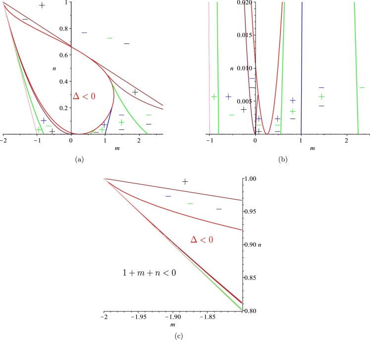
For the set ${\mathrm{\Omega }}_{-}$, we show the curves $\mathrm{\Delta }=0$ and ${\mathrm{C}}_k=0,k=1,2,3$, in Fig. 3.3 (a) with the colors in red, blue, brown and green, respectively. Fig. 3.3(b) is a zoomed area near the m-axis. The region for $\mathrm{\Delta }<0$ is inside the red loop, and $\mathrm{\Delta }>0$ is outside the loop. Thus, we only need to consider the region outside the red loop. We use + or − to indicate ${\mathrm{C}}_k>0$ or ${\mathrm{C}}_k<0$. Fig. 3.3(c) is a zoomed area near the corner of $(m,n)=(-2,1)$, showing that all three curves are tangent to the line $1+m+n=0$ at the corner. This can be rigorously proved using an algebraic argument. Figs. 3.3(a), (b) and (c) clearly show that there are no regions with $\mathrm{\Delta }>0$ and all three functions ${\mathrm{C}}_k>0,k=1,2,3$. Thus, the set ${\mathrm{\Omega }}_{-}$ does not have feasible solutions satisfying $v_1=v_2=0$.

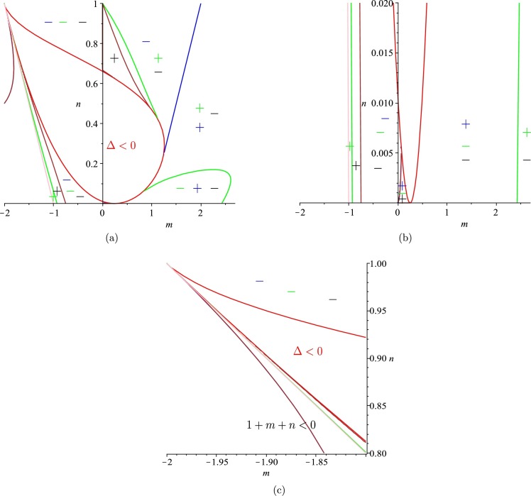
Next, consider the set ${\mathrm{\Omega }}_{+}$. We have a similar result, as shown in Fig. 3.4 . Again, this set also does not have feasible solutions satisfying $v_1=v_2=0$.

To this end, we have shown that under the restrictions on the parameters, as given in (3.25), it is not possible to have solutions such that $v_1=v_2=0$ and to have three limit cycles bifurcating from the equilibrium $(x_0,y_0)=(1,1)$ due to Hopf bifurcation. Therefore, the next best choice is to have $v_1=0$ and $v_2\ne 0$, and P can then be treated as a free parameter. The above proof implies that $v_2$ must be kept the same sign for the feasible parameter values. Otherwise, if it can change sign, then it must have solutions for $v_2=0$, which contradicts the above result. To determine whether the sign of $v_2$ is positive or negative, we only need to choose a solution such that $v_1=0$ and then calculate $v_2$. For example, taking $P=n=m=\frac{1}{10}$, we obtain

$$Q=\frac{35948}{7299}<\frac{(1+P)(1+m+n)-(1-n)P^2}{(1-n)P}=\frac{703741}{72990},$$

giving $v_1=0$ and

$$v_2=\frac{8175332680651336418386743659\sqrt{72884570}}{3491966184311975452303564800000}>0,$$

implying that $v_2>0$ for any parameter values which satisfy the conditions given in (3.25). Thus, the outer bifurcating limit cycle is always unstable and the inner one is stable, both enclose an unstable focus $(1,1)$. The proof is complete. □

Fig. 3.3.

Graphs of the regions on the m-n plane, divided by the curves Δ = C_k = 0, k = 1,2,3: (a) the boundary region 0 < n < 1, 1 + m + n > 0; (b) the zoomed area near the m-axis; and (c) the zoomed area near the corner (m,n)=(−2,1). (For interpretation of the colors in the figure(s), the reader is referred to the web version of this article.)

Fig. 3.4.

Graphs of the regions on the m-n plane, divided by the curves Δ = C_k = 0, k = 1,2,3: (a) the boundary region 0 < n < 1, 1 + m + n > 0; (b) the zoomed area near the m-axis; and (c) the zoomed area near the corner (m,n)=(−2,1).

Remark 3.3

If $m=0$ (i.e., $\beta =0$), then ${\sigma }_{21}=e_0>0$ (i.e., ${\sigma }_2>0$), thus ${\tilde{E}}_2(1,1)$ (i.e., $E_2(x_2,y_2)$) is an unstable multiple focus with multiplicity two when $q=q_2$, $m_3<m<m_4$ and conditions in (3.15) are satisfied. Moreover, when $\beta =0$ (i.e., $m=0$), our system (2.2) is reduced to system (1.2) in [25], where the authors only discussed the Hopf bifurcation of codimension one, thus our results about Hopf bifurcation of codimension two can be seen as a complement of [25] by considering a more general system. On the other hand, when $\beta =0$ (i.e., $m=0$), our system (2.2) also becomes system (1.3) in [27], where the authors showed the existence of degenerate Hopf bifurcation by complex algebraic calculations, our Theorem 3.5, Theorem 3.7 give more explicit conditions and our proofs are easier to follow.

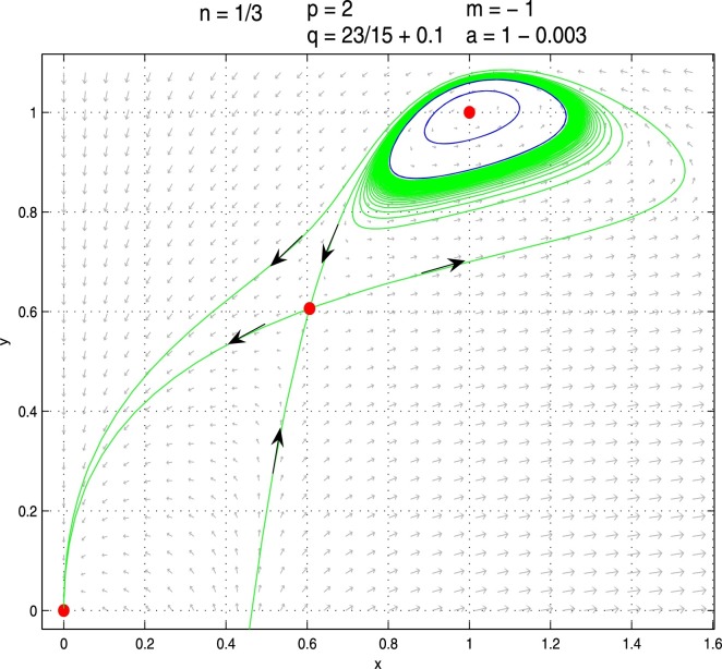
Next we give some numerical simulations in Fig. 3.5 to show the existence of two limit cycles based on Theorem 3.5, Theorem 3.7. Firstly, we fix $n=1/3$, $p=2$ and $m=-1$, then get $q=\frac{23}{15}$ from ${\sigma }_1=0$, and get $a=1$ from $\text{tr}(J({\tilde{E}}_2))=0$, finally get ${\sigma }_2=2.65719$, i.e., ${\tilde{E}}_2(1,1)$ is an unstable multiple focus with multiplicity two for those fixed parameters. Next we first perturb q such that q increases to $\frac{23}{15}+0.1$, then ${\tilde{E}}_2(1,1)$ becomes a stable multiple focus with multiplicity one, an unstable limit cycle occurs around ${\tilde{E}}_2(1,1)$ which is the outer limit cycle in Fig. 3.5. Secondly, we perturb a such that a decreases to $1-0.003$, then ${\tilde{E}}_2(1,1)$ becomes an unstable hyperbolic focus, another stable limit cycle occurs around ${\tilde{E}}_2(1,1)$, which is the inner limit cycle in Fig. 3.5.

Fig. 3.5.

Two limit cycles enclosing an unstable hyperbolic focus in system (3.14) with $n=\frac{1}{3}$, p = 2, m = −1, $q=\frac{23}{15}+0.1$ and a = 1 − 0.003.

Remark 3.4

From Fig. 3.5, we can see that the existence of multiple periodic coexistent oscillations and coexistent steady states when the psychological effect α is smaller than the critical value ${\alpha }_0$ but the infection rate k is greater than the first critical value $k_0$, i.e., $n<n_{⁎}$ and $A>mp$. The disease will die out for almost all initial populations outside the outer unstable periodic orbit, and will tend to periodic outbreaks for almost all initial populations on or inside the outer unstable periodic orbit, and will persist in the form of positive steady states when the initial population lies on the positive equilibria or their stable manifolds.

4. Simulations of the influenza data in Mainland China

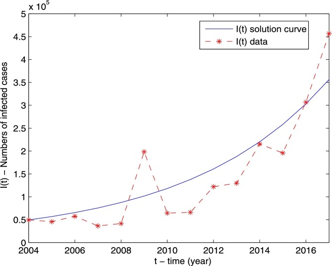
In section 1 we mentioned that nonmonotone and saturated incidence rates may apply to some infectious diseases such as influenza. In this section, we use model (2.1) to simulate the reported human influenza data from China. From the Chinese Center for Disease Control and Prevention (CCDC) [8], we obtain the annual data on human influenza cases from 2004 to 2017 which are shown in Table 1 . Most parameter values can be obtained from the literature or by estimation. We estimate k, α, β, δ and $R(0)$ by using the unconstrained optimization functions $fminsearch$, a part of the optimization toolbox in MATLAB, to fit $I(t_i)$ through discretizing the ordinary differential system (2.1) as follows

$$I(t_i+\mathrm{\Delta }t)=(\frac{kS(t_i)I{(t_i)}^2}{1+\beta I(t_i)+\alpha I{(t_i)}^2}-(d+\mu )I(t_i))\mathrm{\Delta }t+I(t_i).$$

The fitting is to minimize the objective function

$$J(\theta )=\sum _{i=1}^n\frac{{(I(t_i)-\hat{I}(t_i))}^2}{I(t_i)},$$

where $I(t_i)$ is numerical solution of model (2.1) and $\hat{I}(t_i)$ is the reported human influenza data from China.

Table 1.

The data on human influenza cases in China from 2004-2017 ([8]).

Year	2004	2005	2006	2007	2008	2009	2010
Cases	49496	45672	57557	36434	41692	198381	64502

Year	2011	2012	2013	2014	2015	2016	2017
Cases	66133	122140	129873	215533	195723	306682	456718

The parameter values are listed in Table 2 . From the data in 2004, we know that $I(0)=49496$; we make the data fitting to obtain that $R(0)=13$, then $S(0)=1.29983\times {10}^9$; and assume that $\mu =\frac{365}{5}$ from Casagrandi et al. [7], data fitting gives $\delta =0.33042$, $k=2.8668\times {10}^{-8}$, $\alpha =4.9077\times {10}^{-6}$ and $\beta =78.12$.

Table 2.

Parameters of model (2.1).

Para	Value	Unit	Interpretation	Source
b	1.64 × 107	Year−1	human recruitment rate	[23]
d	0.006988	Year−1	human natural mortality rate	[23]
μ	$\frac{365}{5}$	Year−1	human natural recovery rate	[7]
δ	0.33042	Year−1	human loss rate of immunity	fitting
k	2.8668 × 10−8	None	the infection rate	fitting
α	4.9077 × 10−6	None	measures the psychological or inhibitory effect	fitting
β	78.12	None	none	fitting

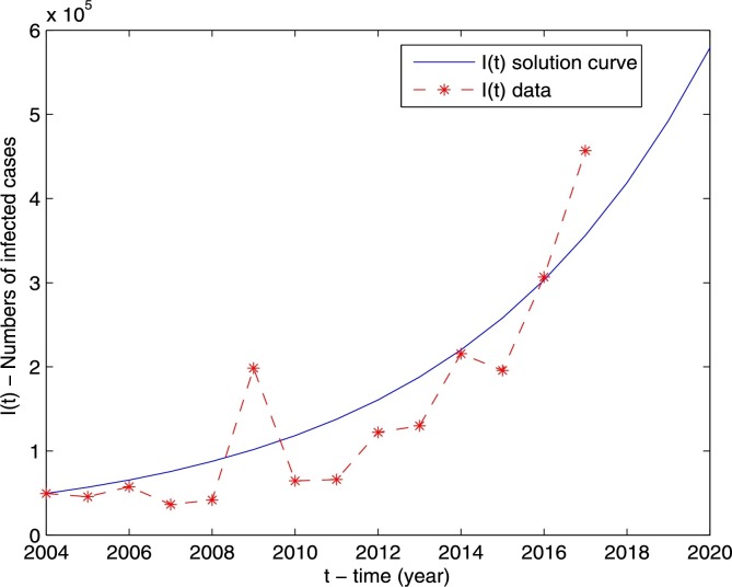
Based on the parameter values given in Table 2, we use model (2.1) to simulate the data from 2004 to 2017 and predict the trend of human influenza infections in China. Fig. 4.1 represents the simulation of our model with reasonable parameter values which provides a good match to the data on infected human influenza cases in China from 2004 to 2017. In Fig. 4.2 our model predicts that the number of human influenza infection will increase in the next a couple of years.

Fig. 4.1.

Simulation of human influenza cases over time in China. The smooth curve represents the solution I(t) of model (2.1) and the dashed curve represents the reported human influenza cases from 2004 to 2017.

Fig. 4.2.

Prediction of human influenza cases in China.

5. Conclusion and discussion

In most classic SIRS epidemic models, the incidence rate is either monotonic or non-monotonic, and the infection force $g(I)$ usually tends to zero as $I\to \infty$ when the incidence rate is non-monotonic, which may be unreasonable for some specific infectious diseases. In this paper, we considered the SIRS epidemic model (1.1) with a generalized nonmonotone and saturated incidence function $g(I)=\frac{k{I}^2}{1+\beta I+\alpha I^2}$, which exhibits three different properties: (i) when $\beta \ge 0$, $g(I)$ is monotonic, which always increases and then tends to a saturated level $\frac{k}{\alpha }$ as I intends to infinite. (ii) When $-2\sqrt{\alpha }<\beta <0$, $g(I)$ is nonmonotonic, which increases when I is small and decreases when I is large, and finally tends to a saturated level $\frac{k}{\alpha }$ as I tends to infinite (see Fig. 1.2), which can be used to describe the phenomenon that the infection force first increases to a maximum when a new infectious disease emerges, and then decreases due to psychological effect and eventually tends to a saturation level due to crowding effect. (iii) When $\beta >-2\sqrt{\alpha }$, $g(I)$ has both properties of (i) and (ii), i.e., $g(I)$ is first nonmonotonic and then monotonic when β increases from negative to positive. In this paper, we performed qualitative and bifurcation analysis, and found that the model (1.1) with general incidence rate (1.8) has complicated dynamical behaviors and bifurcation phenomena. It has been shown that there exists a weak focus of multiplicity at most two and a cusp of codimension at most two for various parameter values, and the model undergoes saddle-node bifurcation, Bogdanov-Takens bifurcation of codimension two, Hopf bifurcation and degenerate Hopf bifurcation of codimension two as the parameter values vary. By considering a more general model, our results show that Bogdanov-Takens bifurcation of codimension higher than two cannot occur, which clarifies and corrects the corresponding results by Tang et al. [27]. Moreover, our results about degenerate Hopf bifurcation (i.e., Hopf bifurcation of codimension two) can also be seen as a complement of the results in Ruan and Wang [25]. We also used model (2.1) to simulate the reported human influenza data from 2004 to 2017 reported by the Chinese Center for Disease Control and Prevention.

In recent years, people realize the importance of the inhibition effect from the behavioral change of susceptible individuals when their number increases or from the crowding effect of the infective individuals, and the psychological effect or inhibition effect can cause people to adopt some aggressive measures and policies, such as border screening, mask wearing, quarantine, isolation and so on, which have been proved to be very effective in reducing the contact rate or the infection force. However, it is difficult to measure the psychological effect. So can we give a quantitative description about the psychological effect with respect to variation of the parameters involved in the infectious diseases? In this paper, we presented a concrete critical value to measure the psychological effect. More specifically, we have shown that there exists a critical value $\alpha ={\alpha }_0$ for the psychological or inhibitory effect and two critical values $k=k_0,k_1(k_0<k_1)$ for the infection rate such that: (i) when $\alpha >{\alpha }_0$, or $\alpha \le {\alpha }_0$ and $k\le k_0$, the disease will die out for all positive initial populations; (ii) when $\alpha ={\alpha }_0$ and $k_0<k\le k_1$, the disease will die out for almost all positive initial populations; (iii) when $\alpha ={\alpha }_0$ and $k>k_1$, the disease will persist in the form of a positive coexistent steady state for some positive initial populations; and (iv) when $\alpha <{\alpha }_0$ and $k>k_0$, the disease will persist in the form of multiple positive periodic coexistent oscillations and coexistent steady states for some positive initial populations.

References

- 1.Alexander M.E., Moghadas S.M. Periodicity in an epidemic model with a generalized nonlinear incidence. Math. Biosci. 2004;189:75–96. doi: 10.1016/j.mbs.2004.01.003. [DOI] [PubMed] [Google Scholar]
- 2.Alexander M.E., Moghadas S.M. Bifurcation analysis of an SIRS epidemic model with generalized incidence. SIAM J. Appl. Math. 2005;65:1794–1816. [Google Scholar]
- 3.Bogdanov R. Bifurcations of a limit cycle for a family of vector fields on the plane. Sel. Math. Sov. 1981;1:373–388. [Google Scholar]
- 4.Bogdanov R. Versal deformations of a singular point on the plane in the case of zero eigen-values. Sel. Math. Sov. 1981;1:389–421. [Google Scholar]
- 5.Capasso V., Crosso E., Serio G. I modelli matematici nella indagine epidemiologica. I Applicazione all'epidemia di colera verificatasi in Bari nel 1973. Ann. Sclavo. 1977;19:193–208. [PubMed] [Google Scholar]
- 6.Capasso V., Serio G. A generalization of the Kermack-McKendrick deterministic epidemic model. Math. Biosci. 1978;42:43–61. [Google Scholar]
- 7.Casagrandi R., Bolzoni L., Levin S., Andreasen V. The SIRC model and influenza A. Math. Biosci. 2006;200:152–169. doi: 10.1016/j.mbs.2005.12.029. [DOI] [PubMed] [Google Scholar]
- 8.http://www.nhfpc.gov.cn/jkj/s3578/new_list.shtml Chinese Center for Disease Control and Prevention, Reports on Infectious Diseases (2004-2017)
- 9.Derrick W.R., van den Driessche P. Homoclinic orbits in a disease transmission model with nonlinear incidence and nonconstant population. Discrete Contin. Dyn. Syst. Ser. B. 2003;3:299–309. [Google Scholar]
- 10.Derrick W.R., van den Driessche P. A disease transmission in a nonconstant population. J. Math. Biol. 1993;31:495–512. doi: 10.1007/BF00173889. [DOI] [PubMed] [Google Scholar]
- 11.Y. Dai, Y. Zhao, B. Sang, Global dynamics for a predator-prey system of Leslie type with generalized Holling type III functional response, submitted for publication.
- 12.Hethcote H.W. The mathematics of infectious disease. SIAM Rev. 2000;42:599–653. [Google Scholar]
- 13.Hethcote H.W., van den Driessche P. Some epidemiological models with nonlinear incidence. J. Math. Biol. 1991;29:271–287. doi: 10.1007/BF00160539. [DOI] [PubMed] [Google Scholar]
- 14.Hu Z., Bi P., Ma W., Ruan S. Bifurcations of an SIRS epidemic model with nonlinear incidence rate. Discrete Contin. Dyn. Syst. Ser. B. 2011;15:93–112. [Google Scholar]
- 15.Huang J., Gong Y., Ruan S. Bifurcation analysis in a predator-prey model with constant-yield predator harvesting. Discrete Contin. Dyn. Syst. Ser. B. 2013;18:2101–2121. [Google Scholar]
- 16.Kermack W.O., McKendrick A.G. A contribution to the mathematical theory of epidemics. Proc. R. Soc. Lond. 1927;115:700–721. [Google Scholar]
- 17.Li J., Zhao Y., Zhu H. Bifurcation of an SIS model with nonlinear contact rate. J. Math. Anal. Appl. 2015;432:1119–1138. [Google Scholar]
- 18.Liu S., Pang L., Ruan S., Zhang X. Global dynamics of avian influenza epidemic models with psychological effects. Comput. Math. Methods Med. 2015;2015 doi: 10.1155/2015/913726. 12 pages. [DOI] [PMC free article] [PubMed] [Google Scholar]
- 19.Liu W.M., Hetchote H.W., Levin S.A. Dynamical behavior of epidemiological models with nonlinear incidence rates. J. Math. Biol. 1987;25:359–380. doi: 10.1007/BF00277162. [DOI] [PubMed] [Google Scholar]
- 20.Liu W., Levin S., Iwasa Y. Influence of nonlinear incidence rates upon the behavior of SIRS epidemiological models. J. Math. Biol. 1986;23:187–204. doi: 10.1007/BF00276956. [DOI] [PubMed] [Google Scholar]
- 21.Lizana M., Rivero J. Multiparametric bifurcations for a model in epidemiology. J. Math. Biol. 1996;35:21–36. doi: 10.1007/s002850050040. [DOI] [PubMed] [Google Scholar]
- 22.Moghadas S.M., Alexander M.E. Bifurcations of an epidemic model with non-linear incidence and infection-dependent removal rate. Math. Med. Biol. 2006;23:231–254. doi: 10.1093/imammb/dql011. [DOI] [PubMed] [Google Scholar]
- 23.http://data.stats.gov.cn/easyquery.htm?cn=C01 National Bureau of Statistics of China (2004-2017)
- 24.Perko L. 3rd ed. Springer; New York: 2001. Differential Equations and Dynamical Systems. [Google Scholar]
- 25.Ruan S., Wang W. Dynamical behavior of an epidemical model with a nonlinear incidence rate. J. Differential Equations. 2003;188:135–163. [Google Scholar]
- 26.Takens F. Forced oscillations and bifurcation. Applications of Global Analysis IComm. Math. Inst. Rijksuniversitat Utrecht. 1974;3:1–59. [Google Scholar]
- 27.Tang Y., Huang D., Ruan S., Zhang W. Coexistence of limit cycles and homoclinic loops in a SIRS model with a nonlinear incidence rate. SIAM J. Appl. Math. 2008;69:621–639. [Google Scholar]
- 28.Wang W. Epidemic models with nonlinear infection forces. Math. Biosci. Eng. 2006;3:267–279. doi: 10.3934/mbe.2006.3.267. [DOI] [PubMed] [Google Scholar]
- 29.Xiao D., Ruan S. Global analysis of an epidemic model with a nonlinear incidence rate. Math. Biosci. 2007;208:419–429. doi: 10.1016/j.mbs.2006.09.025. [DOI] [PMC free article] [PubMed] [Google Scholar]
- 30.Xiao D., Zhou Y. Qualitative analysis of an epidemic model. Can. Appl. Math. Q. 2006;14:469–492. [Google Scholar]
- 31.Yu P. Computation of normal forms via a perturbation technique. J. Sound Vib. 1998;211:19–38. [Google Scholar]
- 32.Zhou Y., Xiao D., Li Y. Bifurcations of an epidemic model with non-monotonic incidence rate of saturated mass action. Chaos Solitons Fractals. 2007;32:1903–1915. doi: 10.1016/j.chaos.2006.01.002. [DOI] [PMC free article] [PubMed] [Google Scholar]
- 33.Zhang Z., Ding T., Huang W., Dong Z. vol. 101. Amer. Math. Soc.; Providence, RI: 1992. Qualitative Theory of Differential Equations. (Transl. Math. Monogr.). [Google Scholar]