A model for the emergence of drug resistance in the presence of asymptomatic infections

Highlights

• •We model the emergence of drug resistance in the presence of asymptomatic cases.
• •The absence of a preclinical state leads to an overestimation of peak incidence.
• •Two reproduction numbers, for drug sensitive or resistant strains, are identified.
• •Drug resistant and sensitive strains can coexist in the population.

Abstract

An analysis of a mathematical model, which describes the dynamics of an aerially transmitted disease, and the effects of the emergence of drug resistance after the introduction of treatment as an intervention strategy is presented. Under explicit consideration of asymptomatic and symptomatic infective individuals for the basic model without intervention the analysis shows that the dynamics of the epidemic is determined by a basic reproduction number $R_0$. A disease-free and an endemic equilibrium exist and are locally asymptotically stable when $R_0<1$ and $R_0>1$ respectively. When treatment is included the system has a basic reproduction number, which is the largest of the two reproduction numbers that characterise the drug-sensitive ($R_1$) or resistant ($R_2$) strains of the infectious agent. The system has a disease-free equilibrium, which is stable when both $R_1$ and $R_2$ are less than unity. Two endemic equilibria also exist and are associated with treatment and the development of drug resistance. An endemic equilibrium where only the drug-resistant strain persists exists and is stable when $R_2>1$ and $R_1<R_2$. A second endemic equilibrium exists when $R_1>1$ and $R_1>R_2$ and both drug-sensitive and drug-resistant strains are present. The analysis of the system provides insights about the conditions under which the infection will persist and whether sensitive and resistant strains will coexist or not.

1. Introduction

A characteristic that influences the transmission dynamics of many infectious diseases is the existence of a subclinical state, where an infected person does not show any symptoms but can, however, spread the infection to other individuals. These, so called, silent spreaders can make a substantial contribution to the transmission of the infectious agent in a population. Therefore, their contribution to the transmission dynamics of an infection should be incorporated into the associated models.

During a disease outbreak, any intervention strategy aimed at mitigating the disease impact is highly dependent on the ability to identify infected individuals, a task which is greatly impeded in the absence of clinical symptoms [1]. In particular, this becomes a vital task for a newly emergent pathogen (e.g. severe acute respiratory syndrome, pandemic influenza), due to the absence of a vaccine in the early stages of the outbreak. Policy decisions for public health planning rely on early estimates of disease parameters, however, unreported subclinical cases lead to difficulties in accurately estimating the basic reproduction number of the disease [2]. The resultant uncertainty in epidemiological models greatly hinders the decision making process and casts doubt on the effectiveness of proposed interventions. The presence of subclinical infections in a population can significantly influence the outcome of non-pharmaceutical interventions, for example monitoring international borders for symptomatic travellers can be undermined as asymptomatic individuals are impossible to identify using standard methods [3]. Furthermore, isolating and/or treating clinical cases may be inadequate to protect vulnerable populations from the further spread of disease. Prophylaxis of exposed populations can be a useful intervention, in particular, when a vaccine needs time to be developed. However, the possibility of drug resistance as a byproduct of the treatment process is an undesirable, but potential, side effect and its epidemiological impact and the likelihood of transmission of drug-resistant infectious agents need to be studied closer.

Subclinical infections are typically modelled using two approaches. The first separates the infectious population into asymptomatic and symptomatic states immediately following the onset of infectiousness [4], [5], [6]. However, not all diseases follow such a straightforward path and, in particular, the relative durations of the latent and incubation periods should be considered. For certain diseases, a more appropriate model may allow for a preclinical state where an asymptomatic infectious state precedes the onset of clinical symptoms, Fig. 1 . Such a model has been used in the context of influenza where the incubation period is believed to exceed the duration of the latent state [7], [8], [9], [10], [11], [12].

Fig. 1.

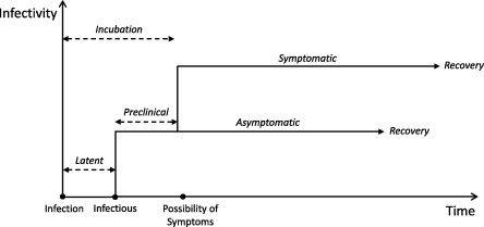
Disease pathway.

In this paper we present some features of a mathematical model for aerially transmitted diseases (e.g. meningitis, influenza, staphylococcus aureus). In the model there are two classes of infected, and thus infectious, individuals; those who develop symptoms after an asymptomatic period and those who remain asymptomatic but infectious and recover without having passed through the symptomatic state. We provide a comparison with an alternative widely-used model which neglects the existence of a preclinical infectious state. We investigate the same features in a modified version of the model, where treatment is applied as an intervention strategy and the resultant development of drug resistance as a side effect is evaluated. Both models are based on a previously developed model for the emergence of drug resistance during influenza epidemics under explicit consideration of asymptomatic cases [7]. We now generalise that model for any persistent infectious disease with infectious asymptomatic cases and in addition we elaborate on the dynamics when treatment is used as intervention strategy.

2. The basic model

The total population $N(t)$ is divided into four distinct classes such that $N(t)=s(t)+i_A(t)+i_S(t)+r(t)$, where $s(t)$ denotes the number of susceptible individuals at time $t$, $i_A(t)$ the number of asymptomatic infectives, $i_S(t)$ the number of symptomatic infectives and $r(t)$ the number of recovered people. The infection is transmitted to a susceptible person through contact with either a symptomatic or asymptomatic infected person. Once infected, all susceptible individuals enter an asymptomatic state, indicating a delay between infectiousness and symptom onset. From here, an individual can either progress to the symptomatic state of infection or recover without ever developing symptoms. It is assumed that there are no disease related deaths and all infected individuals eventually recover. We further assume that recovered individuals do not obtain lifelong immunity to infection. This assumption incorporates the antigenic drift of some infectious agents, such as influenza, which results in previously infected individuals becoming susceptible to the virus again. The transition diagram for the infection pathway is shown in Fig. 2 and the model is described by the system of equations

$$\begin{array}{cc}\hfill & \frac{\mathit{ds}}{\mathit{dt}}=\mathrm{\Lambda }+\alpha r-\mu s-({\beta }_A{i}_A+{\beta }_S{i}_S)\frac{s}{N}\text{,}\hfill \\ \hfill & \frac{{\mathit{di}}_A}{\mathit{dt}}=({\beta }_A{i}_A+{\beta }_S{i}_S)\frac{s}{N}-(\delta +{\gamma }_A+\mu )i_A\text{,}\hfill \\ \hfill & \frac{{\mathit{di}}_S}{\mathit{dt}}=\delta i_A-({\gamma }_S+\mu )i_S\text{,}\hfill \\ \hfill & \frac{\mathit{dr}}{\mathit{dt}}={\gamma }_A{i}_A+{\gamma }_S{i}_S-(\mu +\alpha )r\text{,}\hfill \end{array}$$

where $\mathrm{\Lambda }$ and $\mu$ are the constant birth and natural death rates respectively. We assume all infected individuals eventually recover, losing their acquired immunity after a period of $1/\alpha$ days and return to the susceptible class. The transition rates associated with asymptomatic and symptomatic individuals are ${\beta }_A$ and ${\beta }_S$ respectively. Following the onset of symptoms, the average time to recovery is $1/{\gamma }_S$ days. For an asymptomatic case two scenarios are possible. An individual may remain asymptomatic for the duration of the infection and recover after $1/{\gamma }_A$ days. Alternatively, an individual may remain asymptomatic (preclinical) for a shorter period of $1/\delta$ days before ultimately developing symptoms. Therefore, the average residence time in the $I_A$ class is $1/(\delta +{\gamma }_A+\mu )$.

Fig. 2.

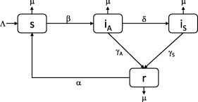
Transition diagram for SIRS model with asymptomatic and symptomatic disease states.

The limiting case $\delta \to 0$, yields a standard SIRS model for a silent (asymptomatic) infection [13]. In contrast, the asymptomatic state becomes redundant in the limit $\delta \to \infty$, which corresponds to individuals spending an infinitely short time in the asymptomatic stage and again results in a standard SIRS model for a purely symptomatic infection. Symptomatic individuals, on coming in contact with susceptible individuals, transmit the infection more readily than asymptomatic individuals due to physical signs of illness (coughing, sneezing, etc.). However, asymptomatic individuals will presumably have more contacts since lack of symptoms implies a lack of self-induced quarantine [14]. We assume that the first effect outweighs the second and take ${\beta }_S=c{\beta }_A$, with $c>1$.

The change in the total population size follows

$$\frac{\mathit{dN}}{\mathit{dt}}=\frac{\mathit{ds}}{\mathit{dt}}+\frac{{\mathit{di}}_A}{\mathit{dt}}+\frac{{\mathit{di}}_S}{\mathit{dt}}+\frac{\mathit{dr}}{\mathit{dt}}=\mathrm{\Lambda }-\mu N\text{,}$$

and the total population then develops via

$$N(t)=\frac{\mathrm{\Lambda }}{\mu }+\left(N(0)-\frac{\mathrm{\Lambda }}{\mu }\right)e^{-\mu t}\text{,}$$

with N approaching the limiting value $N_{\infty }=\mathrm{\Lambda }/\mu$. We assume that the population is approximately constant over the infection timescale and we set $\mathrm{\Lambda }=\mu N$ yielding a constant population size where births balance natural deaths. The constant population assumption also allows us to write $r(t)=N-(s(t)+i_A(t)+i_S(t))$ and eliminate the equation for r from the analysis. It is convenient to scale each compartment with the total population so that the resulting variables represent the proportion of the total population in each compartment. The model now becomes

$$\frac{\mathit{dS}}{\mathit{dt}}=\mu (1-S)+\alpha (1-S-I_A-I_S)-({\beta }_A{I}_A+{\beta }_S{I}_S)S\text{,}$$ (1)

$$\frac{{\mathit{dI}}_A}{\mathit{dt}}=({\beta }_A{I}_A+{\beta }_S{I}_S)S-(\delta +{\gamma }_A+\mu )I_A\text{,}$$ (2)

$$\frac{{\mathit{dI}}_S}{\mathit{dt}}=\delta I_A-({\gamma }_S+\mu )I_S\text{,}$$ (3)

and the fraction of recovered individuals is determined from $R=1-(S+I_A+I_S)$. Equilibria of the system (1), (2), (3) are obtained by setting the right-hand side of each of the equations equal to zero. Clearly the point $P^0=(1\text{,}0\text{,}0)$ is a solution and represents a disease-free state. The disease-free equilibrium can be used to determine the basic reproduction number. It represents the average number of secondary infections arising from an average primary infection in an entirely susceptible population [15]. It can be explicitly derived by calculating the next generation matrix using the methods outlined in [16], [17], [18], [19]. The basic reproduction number is given by the largest eigenvalue of this matrix which is found to be

$$R_0=R_A+R_S\text{,}$$

where

$$R_A=\frac{{\beta }_A}{\delta +{\gamma }_A+\mu }\text{,}{R}_S=\frac{{\beta }_s\delta }{(\delta +{\gamma }_A+\mu )({\gamma }_S+\mu )}\text{.}$$

The spread of infection can be viewed as a series of linked subepidemics. One subepidemic will be driven by infections caused through contact with subclinically infected individuals (${\beta }_S=0$) with a reproduction number $R_A$ and another driven by infection through contact with clinically infected individuals (${\beta }_A=0$) with a reproduction number $R_S$. In practice, it is extremely difficult to estimate transmission rates for an epidemic in progress. However, the basic reproduction number can be determined from disease incidence data. Accordingly, $R_0$ is effectively a known parameter from which the transmission rate ${\beta }_A$ can be determined, and the symptomatic transmission rate is calculated from ${\beta }_S=c{\beta }_A$, where

$${\beta }_A=\frac{(\delta +{\gamma }_A+\mu )({\gamma }_S+\mu )}{({\gamma }_S+\mu +c\delta )}{R}_0\text{.}$$ (4)

Now in addition to the disease-free equilibrium $P^0$, the system also possesses an endemic state $P^e$ given by

$$S^e=\frac{1}{R_0}\text{,}$$ (5)

$$I_A^e=\frac{({\gamma }_S+\mu )(\mu +\alpha )}{\alpha ({\gamma }_S+\mu )+\alpha \delta +(\delta +{\gamma }_A+\mu )({\gamma }_S+\mu )}\left(1-\frac{1}{R_0}\right)\text{,}$$ (6)

$$I_S^e=\frac{\delta (\mu +\alpha )}{\alpha ({\gamma }_S+\mu )+\alpha \delta +(\delta +{\gamma }_A+\mu )({\gamma }_S+\mu )}\left(1-\frac{1}{R_0}\right)\text{.}$$ (7)

When $0<R_0<1$ the infected populations become negative and the equilibrium point is no longer biologically feasible. When $R_0=1$ the endemic state merges with the disease-free state to yield a single equilibrium. When $R_0>1$ both equilibria exist.

2.1. Local stability analysis

Following the results outlined in [16], the disease-free equilibrium $P^0$ of the system (1), (2), (3) will be locally asymptotically stable when $R_0<1$. To determine the stability of the endemic equilibrium $P^e$, given by (5), (6), (7), the Jacobian matrix is evaluated at this point

$$J{|}_{P^e}=\left[\begin{array}{ccc}\hfill -{\mathrm{\Omega }}_0-\frac{{\mathrm{\Omega }}_0{\mathrm{\Omega }}_1{\mathrm{\Omega }}_2}{M}(R_0-1)\hfill & \hfill -\alpha -\frac{{\beta }_A}{R_0}\hfill & \hfill -\alpha -\frac{{\beta }_S}{R_0}\hfill \\ \hfill \frac{{\mathrm{\Omega }}_0{\mathrm{\Omega }}_1{\mathrm{\Omega }}_2}{M}(R_0-1)\hfill & \hfill \frac{{\beta }_A}{R_0}-{\mathrm{\Omega }}_1\hfill & \hfill \frac{{\beta }_S}{R_0}\hfill \\ \hfill 0\hfill & \hfill \delta \hfill & \hfill -{\mathrm{\Omega }}_2\hfill \end{array}\right]\text{,}$$

where, for convenience, we have set

$$\begin{array}{cc}\hfill & {\mathrm{\Omega }}_0=\alpha +\mu \text{,}\hfill \\ \hfill & {\mathrm{\Omega }}_1=\delta +{\gamma }_A+\mu \text{,}\hfill \\ \hfill & {\mathrm{\Omega }}_2={\gamma }_S+\mu \text{,}\hfill \\ \hfill & M=\alpha {\mathrm{\Omega }}_2+\alpha \delta +{\mathrm{\Omega }}_1{\mathrm{\Omega }}_2\text{.}\hfill \end{array}$$

The characteristic equation is the cubic polynomial $F(\lambda )={\sum }_{i=0}^3{f}_i{\lambda }^i$ with coefficients

$$\begin{array}{cc}\hfill & f_3={\mathit{MR}}_0\text{,}\hfill \\ \hfill & f_2={\mathrm{\Omega }}_0{\mathrm{\Omega }}_1{\mathrm{\Omega }}_2{R}_0(R_0-1)+{\mathit{MR}}_0({\mathrm{\Omega }}_0+{\mathrm{\Omega }}_1+{\mathrm{\Omega }}_2)-M{\beta }_A\text{,}\hfill \\ \hfill & f_1={\mathrm{\Omega }}_0{\mathrm{\Omega }}_1{\mathrm{\Omega }}_2{R}_0(\alpha +{\mathrm{\Omega }}_1+{\mathrm{\Omega }}_2)(R_0-1)+{\mathit{MR}}_0{\mathrm{\Omega }}_0({\mathrm{\Omega }}_1+{\mathrm{\Omega }}_2)-M{\mathrm{\Omega }}_0{\beta }_A\text{,}\hfill \\ \hfill & f_0=M{\mathrm{\Omega }}_0{\mathrm{\Omega }}_1{\mathrm{\Omega }}_2{R}_0(R_0-1)\text{,}\hfill \end{array}$$

and stability requires

$$f_0{f}_3>0\text{,}{f}_2{f}_3>0\text{,}{f}_1{f}_2-f_0{f}_3>0\text{.}$$

Clearly $f_0>0$ when $R_0>1$. In any case, this condition must be satisfied for $P^e$ to exist. The second inequality can be written as

$$R_0>1-\frac{{\mathit{MT}}_2({\mathrm{\Omega }}_0+{\mathrm{\Omega }}_2)+c\delta M({\mathrm{\Omega }}_0+{\mathrm{\Omega }}_1+{\mathrm{\Omega }}_2)}{{\mathrm{\Omega }}_0{\mathrm{\Omega }}_1{\mathrm{\Omega }}_2({\mathrm{\Omega }}_2+c\delta )}\text{,}$$

which is always satisfied when $R_0>1$. Finally, the third inequality can be written in the form

$$f_1{f}_2-f_0{f}_3={\mathrm{\Omega }}_0{\mathrm{\Omega }}_1{\mathrm{\Omega }}_2{R}_0(R_0-1)\left[\frac{(\alpha +{\mathrm{\Omega }}_1+{\mathrm{\Omega }}_2)}{{\mathrm{\Omega }}_2}\left[M{\beta }_S\delta +{\mathrm{\Omega }}_0{\mathrm{\Omega }}_1{\mathrm{\Omega }}_2^2{R}_0(R_0-1)\right]+{\mathit{MR}}_0\left[{\mathrm{\Omega }}_2^2+{\mathrm{\Omega }}_0(\alpha +{\mathrm{\Omega }}_2)+\mu {\mathrm{\Omega }}_1+\alpha ({\gamma }_A+\mu )\right]\right]+\frac{f_{2}M{\mathrm{\Omega }}_0}{{\mathrm{\Omega }}_2}\left[{\beta }_S\delta +R_0{\mathrm{\Omega }}_2^2\right]>0\text{.}$$

Hence, the endemic equilibrium $P^e$ is always locally asymptotically stable. The existence and stability of the equilibria is completely determined by the threshold parameter $R_0$. The disease-free equilibrium exists for all $R_0$, is stable when $R_0<1$ and unstable when $R_0>1$. The endemic equilibrium exists only for $R_0>1$ and is always stable. This is an example of a transcritical bifurcation. As $R_0$ crosses unity from below the disease-free equilibrium loses its stability and a positive asymptotically stable endemic equilibrium appears. The forward bifurcation is shown in Fig. 3 , where we plot the steady state value of S as a function of $R_0$.

Fig. 3.

Bifurcation diagram showing how the steady state value of S varies with $R_0$.

2.2. An alternative modelling approach

As discussed in the introduction, another model commonly used to describe an asymptomatic-symptomatic infection neglects the possibility of a preclinical state, with the instantaneous development of clinical illness following the onset of infectiousness. In addition, this model assumes that all asymptomatically infected individuals recover without ever developing symptoms. We believe this is an oversimplification of the disease pathway for many infections (e.g. influenza). In this section we investigate the impact of neglecting the preclinical state on disease dynamics. For clarity, we will refer to this model as Model II. The alternative system of equations is given by

$$\frac{\mathit{dS}}{\mathit{dt}}=\mu (1-S)+\alpha (1-S-I_A-I_S)-({\beta }_A{I}_A+{\beta }_S{I}_S)S\text{,}$$ (8)

$$\frac{{\mathit{dI}}_A}{\mathit{dt}}=(1-p)({\beta }_A{I}_A+{\beta }_S{I}_S)S-({\gamma }_A+\mu )I_A\text{,}$$ (9)

$$\frac{{\mathit{dI}}_S}{\mathit{dt}}=p({\beta }_A{I}_A+{\beta }_S{I}_S)S-({\gamma }_S+\mu )I_S\text{,}$$ (10)

where all variables and parameters are defined as before and p denotes the proportion of infected individuals who develop symptoms. The two limiting cases of a solely asymptomatic or symptomatic infection occur in the limits $p\to 0$ and $p\to 1$ respectively. In fact, the two models are identical when $p=\delta =0$ or in the limit $\delta \to \infty$ with $p=1$. The average residence time in the asymptomatic state differs in both models, with Model II yielding a longer residence time of $1/({\gamma }_A+\mu )$.

As in the previous case, we can obtain an expression for the basic reproduction number from the next generation matrix,

$$R_0=R_A+R_S=(1-p)\frac{{\beta }_A}{{\gamma }_A+\mu }+p\frac{{\beta }_S}{{\gamma }_S+\mu }\text{,}$$

where $R_A$ and $R_S$ describe the contributions to the initial epidemic growth of each infectious (asymptomatic/symptomatic) state. The basic reproduction number is a characteristic of the disease and can be estimated from incidence date. In contrast, it is all but impossible to estimate the transmission rate and, accordingly, $R_0$ is fixed and the above expression is used to determine the transmission rate for Model II,

$${\beta }_A^{\mathit{II}}=\frac{({\gamma }_A+\mu )({\gamma }_S+\mu )}{(1-p)({\gamma }_S+\mu )+\mathit{cp}({\gamma }_A+\mu )}{R}_0\text{,}$$ (11)

where it is assumed that ${\beta }_S^{\mathit{II}}=c{\beta }_A^{\mathit{II}}$. On comparison with the transmission rate for the basic model (4) we see that, with all other parameters fixed by the observed disease dynamics, the two models yield unique transmission rates. So that, for a fixed value of $R_0$, the two models will yield different transmission rates. For clarity, we denote the transmission rates of Model II as ${\beta }_A^{\mathit{II}}$ and ${\beta }_S^{\mathit{II}}$ and the corresponding asymptomatic and symptomatic reproduction numbers as $R_A^{\mathit{II}}$ and $R_S^{\mathit{II}}$ respectively.

The transmission rate contains information about the contact structure within the population and its value will depend on the partitioning of the population into the different disease states. The two models distribute the infected population differently, determined by the parameters p and $\delta$, and we propose that this can lead to two distinct transmission rates. To compare the two models we write ${\beta }_A^{\mathit{II}}=F(\delta \text{,}p){\beta }_A$ where

$$F(\delta \text{;}p)=\frac{({\gamma }_A+\mu )({\gamma }_S+\mu +c\delta )}{(\delta +{\gamma }_A+\mu )[(1-p)({\gamma }_S+\mu )+\mathit{cp}({\gamma }_A+\mu )]}\text{,}$$ (12)

which contains the information about the different distribution of cases between the two models. Identical transmission rates, corresponding to $F(\delta \text{;}p)=1$, are achieved in the two limiting cases of a purely asymptomatic ($\delta =p=0$) or symptomatic ($p=1$ and $\delta \to \infty$) infection. In addition, it can be easily shown that

$$F\left({\delta }_c\text{;}p\right)=1\text{,}\text{where}{\delta }_c=\frac{p}{1-p}({\gamma }_A+\mu )\text{.}$$ (13)

2.3. The case of influenza

The recent influenza 2009 H1N1 pandemic has heightened the need for public health authorities to have pandemic preparedness plans in place in advance of a future outbreak. However, the presence of silent spreaders, in the form of asymptomatically infected individuals, can severely undermine potential control strategies. In particular, such individuals can have a profound impact on immunologically naive or compromised populations, such as those in schools and health care facilities, where unavoidable close contact encounters can lead to the rapid spread of an infection. Disease transmission by asymptomatic individuals was documented in such settings during the 2009 outbreak [20], [21]. Furthermore, viral shedding during the preclinical stage of infection was confirmed to occur in approximately 1–8% of infections [22] and preclinical transmission was also recorded in early H1N1 outbreaks [23]. Mathematical models have demonstrated how preclinical transmission can influence the magnitude of outbreaks in large closed populations, such as schools, workplaces and military facilities, and highlights the importance of such transmission in the decision process [24]. In particular, a greater transmission ability during the preclinical period has been associated with children [25] and this increases the need to understand the effects of this state on the disease pathway. In this section we investigate the behaviour of the two models previously discussed for the specific case of the influenza virus. In particular, we consider the impact of a simple public health intervention applicable to large closed populations, where the easily identifiable clinical cases are isolated from the general population.

To parameterise the model we take the average human lifespan to be 70 years, with infection acquired immunity being lost after a period of 1 year. The degree to which asymptomatic individuals contribute to transmission is uncertain. Existing mathematical models assume the relative transmission from an asymptomatic case is from as little as one tenth [7], [8], [9] to as high as twice [26] that of a symptomatic case. However, while it is widely acknowledged that asymptomatic infection is common, the ability of such individuals to efficiently transmit has been questioned, due to the low levels of viral shedding in such cases [22], [27], [28]. So as not to overestimate the asymptomatic contribution we take the value $c=10$. For modelling purposes, the proportion of infected individuals developing symptoms is commonly taken as approximately two thirds [4], [5], [29]. Justification for this choice is rarely provided, however, a recent review of experimental studies in which volunteer exposure to wild-type influenza virus was examined determined that the frequency of symptom development was 66.9% [30]. We adopt this assumption and set $p=0.67$.

The course of infection for influenza is not fully understood. The primary uncertainty surrounds the incubation period and the possibility that it is longer than the latent period resulting in asymptomatic individuals who are infectious [1]. A mean incubation period of 2.05 days was estimated from laboratory confirmed cases of H1N1 in the United Kingdom [31]. Viral shedding has been detected on average one day after inoculation with the influenza virus indicating that a latent period of approximately 1 day precedes the onset of infectiousness [30]. Accordingly, the duration of the preclinical infectious state is approximately 1 day and we take $\delta =1$  day⁻¹, in agreement with experimental observations [30]. We neglect the latent period in our analysis as it essentially introduces a delay into the system and rarely results in qualitatively different dynamics [13], [15]. Infected individuals are commonly assumed to recover from clinical illness after an average period of 4 days and we set ${\gamma }_S=0.25$  day⁻¹ [4], [32], [33]. This estimate is predominantly derived from studies that estimate the average duration of viral shedding and represents a rather conservative estimate. One could also use values derived from estimates of the mean serial interval, which in general have been somewhat lower, approximately 3 days, depending on the viral strain [33]. The duration of infectiousness for an asymptomatic case is unknown but previous modelling studies have taken it to be half that of a symptomatic case [34], [35] and we also adopt this assumption, taking ${\gamma }_A=0.5$  day⁻¹. The choice of a 2 day duration for the asymptomatic state yields a probability of progressing to a symptomatic state given by $\delta /({\gamma }_a+\delta +\mu )\approx 0.67$, in agreement with the corresponding probability in Model II of $p=0.67$. With the above choice of parameters, the average residence times in the asymptomatic state predicted by the basic model and Model II are approximately 2/3 day and 2 days respectively. It should be noted that, although the basic model yields a significantly shorter residence time, all infected individuals pass through this state and are capable of eluding intervention attempts while preclinical and silently spreading the infection within a susceptible population.

The basic reproduction number can vary significantly between different pandemic and seasonal outbreaks. Estimates for the 2009 H1N1 pandemic are in the range 1.3–1.7 [36] and an average seasonal value is approximately 1.3 [37] and we take this value in our simulations. The parameter choices discussed above yield identical transmission rates for the two models since ${\delta }_c\approx 1$  day⁻¹ from (13) and, thus, $F(1\text{,}0.67)=1$ in (12). All parameters and the values used in numerical simulations are listed in Table 1 .

Table 1.

Parameter values used in the model.

Parameters		Values for influenza	Reference
N	Population	${10}^4$	Estimated
$\mu$	Per-capita natural death rate	$\frac{1}{70\times 365}$ day−1	Estimated
$\alpha$	Rate at which immunity is lost	$\frac{1}{365}$ day−1	Estimated
p	Proportion of infected who develop symptoms	0.67	[30]
$\delta$	Inverse of preclinical duration	1 day−1	[30]
${\delta }_r$	Inverse of preclinical duration for resistant strain	1 day−1	Estimated
${\gamma }_A$	Recovery rate from asymptomatic infection	0.5 day−1	[34], [35]
${\gamma }_S$	Recovery rate from symptomatic infection	0.25 day−1	[4], [32]
$\sigma$	Rate that infected are identified and isolated	0.05 day−1	Estimated
$\theta$	Treatment rate of $I_S$ and $I_{S\text{,}r}$	0.7 day−1	Estimated
$\rho$	Relative infectivity of $I_{S\text{,}\mathit{tr}}$ compared with $I_S$	0.67	[39], [40]
r	Relative recovery of $I_{S\text{,}\mathit{tr}}$ compared with $I_S^a$	1.5	[8]
q	Probability of emergence of acquired drug resistancea	0.01	[41]
$\eta$	Rate of drug resistance development during treatmenta	0.2 day−1	[42]
c	Increased infectivity of symptomatic infections	10	[7], [8], [9]
$R_0$	Basic reproduction numberb	1.3	[37]

Note: Transmission rates for the treatment model are calculated using the values of $R_1$ and $R_2$ indicated in the caption of the relevant figure.

^aValues given are for treatment with neuraminidase inhibitors.

^bTransmission rates are calculated from this value using (4), (11).

The solution for the infected populations of both models, with initial conditions $S(0)=1-1/N$, $I_A(0)=0$ and $I_S(0)=1/N$, is plotted in Fig. 4 . This initial condition corresponds to one symptomatically infected person in a completely susceptible population of size $N-1$. A population of $N={10}^4$ is taken in all simulations. The solutions are qualitatively similar, however, Model II yields a higher peak incidence. Significantly, identical transmission rates does not produce quantitatively identical disease incidence and the partitioning of the population into unique disease states is an important factor in the modelling process. In fact, there will still be differences between the models in the generation time, as well in several other quantities, such as the expected number of cases generated by an asymptotic individual. The delay observed in the basic model is invariably due to the delay introduced by all newly infected individuals being required to first pass through the asymptomatic state prior to symptom onset and the reduced transmission therein. The reverse occurs when the initial infectious seed is asymptomatic. The solution with initial conditions $S(0)=1-1/N$, $I_A(0)=1/N$ and $I_S(0)=0$ is plotted in Fig. 5 . Under this scenario, the delay in symptomatic cases is observed to occur in Model II. This can be attributed to the relatively small transmission potential of the asymptomatic cases and the resultant time taken for the infection to gain a foothold in the population. Whereas, some of the initially asymptomatic individuals in the basic model quickly transition to the symptomatic cases and can start transmitting the infection more efficiently.

Fig. 4.

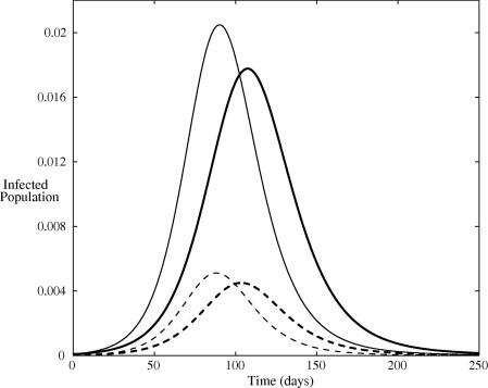
Infected population predicted by the two models. The dark and pale lines denote the solution of the basic model and Model II respectively. Solid lines indicate symptomatic infections and dashed lines indicate asymptomatic infections. All parameters are listed in Table 1 and initial conditions are $S(0)=0.99$, $I_A(0)=0$ and $I_S(0)=0.01$.

Fig. 5.

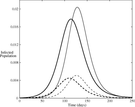
Infected population predicted by the two models. The dark and pale lines denote the solution of the basic model and Model II respectively. Solid lines indicate symptomatic infections and dashed lines indicate asymptomatic infections. All parameters are listed in Table 1 and initial conditions are $S(0)=0.99$, $I_A(0)=0.01$ and $I_S(0)=0$.

The impact of the duration of the preclinical state on the epidemic growth can be analysed by considering the relative contributions of each infectious state for varying $\delta$, Fig. 6 . It is clear that $R_A\to R_0$ and $R_S\to 0$ as $\delta \to 0$ and the only contribution to the basic reproduction number comes from the asymptomatic population, as expected with a silent infection. Similarly, $R_S\to R_0$ and $R_A\to 0$ as $\delta \to \infty$ indicating the sole presence of symptomatic individuals. When $\delta <1$ the basic model predicts a larger $R_A$ and smaller $R_S$ than Model II. This implies that, when the duration of the preclinical state exceeds 1 day, asymptomatic infections make a more significant contribution in the basic model and Model II may underestimate their contribution to the initial epidemic growth. Conversely, when $\delta >1$, corresponding to a preclinical state of less than 1 day, the basic model predicts a smaller $R_A$ and larger $R_S$ than Model II, with the greater contribution coming from the symptomatic cases, since the average residence time spent in the asymptomatic state decreases as $\delta$ increases.

Fig. 6.

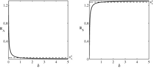
A comparison of asymptomatic and symptomatic reproduction numbers for the two models. The dashed line indicates the ($\delta$-independent) values for Model II and the solid line denotes the basic model. All parameters are listed in Table 1.

To investigate the consequences of the different population partitionings adopted by the two models we consider the implementation of one of the simplest public health interventions, whereby symptomatic individuals are isolated from the general population. The models can be easily adapted to incorporate this process by removing symptomatic individuals at the rate $\sigma$ that they are identified and placed in isolation. The proportion of isolated cases Q at time t will then satisfy the differential equation

$$\frac{\mathit{dQ}}{\mathit{dt}}=\sigma I_S-({\gamma }_S+\mu )Q\text{,}$$

where isolated individuals recover and rejoin the general population after an average of $1/{\gamma }_S$ days. The transmission term must also be modified to account for the fact that the fraction of infectious contacts changes from $I/N$ to $I/(N-Q)$.

The results of the introduction of isolation as an intervention measure are qualitatively similar to before, Fig. 7, Fig. 8 . As expected, the peak severity of the outbreak is reduced and a delay is again observed between the two model solutions. However, the duration of the outbreak is extended and, in particular, the delay observed between the peak incidence of both models is significantly increased. In the case of a symptomatic initial seed, the delay in symptomatic cases increases from approximately 17 days (Fig. 4) to 33 days (Fig. 7) when isolation is present. If the initial seed is asymptomatic then this delay increases almost fourfold from 14 days to 55 days. Therefore, the different partitions of the asymptomatic population in the two infection models can produce very different results which could potentially interfere with the design and implementation of intervention strategies. More biologically realistic models can aid public health systems to effectively manage disease outbreaks.

Fig. 7.

Infected population predicted by the two models with isolation of clinical cases. The dark and pale lines denote the solution of the basic model and Model II respectively. Solid lines indicate symptomatic infections and dashed lines indicate asymptomatic infections. All parameters are listed in Table 1 and initial conditions are $S(0)=1-1/N$, $I_A(0)=0$ and $I_S(0)=1/N$.

Fig. 8.

Infected population predicted by the two models with isolation of clinical cases. The dark and pale lines denote the solution of the basic model and Model II respectively. Solid lines indicate symptomatic infections and dashed lines indicate asymptomatic infections. All parameters are listed in Table 1 and initial conditions are $S(0)=1-1/N$, $I_A(0)=1/N$ and $I_S(0)=0$.

2.4. Long term behaviour

If we consider the long term behaviour of both models, when the repopulation of the susceptible class through births and loss of immunity becomes important, we find the basic model approaches the endemic equilibrium given by (5), (6), (7). Model II approaches the endemic equilibrium $P^{e^{\mathit{II}}}$ where

$$\begin{array}{cc}\hfill & S^{e^{\mathit{II}}}=\frac{1}{R_0}\text{,}\hfill \\ \hfill & I_A^{e^{\mathit{II}}}=\frac{(1-p)({\gamma }_S+\mu )(\alpha +\mu )}{\alpha p({\gamma }_A+\mu )+({\gamma }_A+\mu )({\gamma }_S+\mu )+\alpha (1-p)({\gamma }_S+\mu )}\left(1-\frac{1}{R_0}\right)\text{,}\hfill \\ \hfill & I_S^{e^{\mathit{II}}}=\frac{p({\gamma }_A+\mu )(\alpha +\mu )}{\alpha p({\gamma }_A+\mu )+({\gamma }_A+\mu )({\gamma }_S+\mu )+\alpha (1-p)({\gamma }_S+\mu )}\left(1-\frac{1}{R_0}\right)\text{,}\hfill \end{array}$$

which exists when $R_0>1$. It can be easily shown that the two endemic equilibria are equal. Thus, the long-term behaviour of the two models is identical but the short term oscillations are out of phase with each other, Fig. 9 . The reason for this delay was discussed in the previous section. The endemic equilibria as a function of $\delta$ are plotted in Fig. 10 . The equilibria coincide when $\delta ={\delta }_c=1$. When $\delta <1$, and the duration of the preclinical state exceeds 1 day, the basic model predicts a larger endemic value for $I_A$ and a smaller value for $I_S$. The opposite is true when the preclinical state is shorter than 1 day, $\delta >1$. This indicates that, in the long term behaviour of influenza, the disease burden could be over or under estimated if the duration of the preclinical state is not accurately known. Better estimates of this parameter could yield more reliable predictions.

Fig. 9.

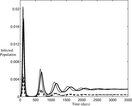
Long term infected population predicted by the two models. The dark and pale lines denote the solution of the basic model and Model II respectively. Solid lines indicate symptomatic infections and dashed lines indicate asymptomatic infections. All parameters are listed in Table 1 and initial conditions are $S(0)=0.99$, $I_A(0)=0$ and $I_S(0)=0.01$.

Fig. 10.

A comparison of the endemic equilibria $P^e$ and $P^{e^{\mathit{II}}}$ for the two models. The dashed line indicates the ($\delta$-independent) values for Model II and the solid line denotes the basic model. All parameters are listed in Table 1.

Deterministic models with vital dynamics have been shown to exhibit damped oscillations about an endemic disease state for childhood diseases [13], [15]. Influenza has a relatively short infectious period and small reproduction number compared with such infections (measles, rubella, etc.). As a consequence, the disease dynamics of influenza are sufficiently rapid that vital dynamics are typically neglected as they are inadequate to replenish the pool of susceptible individuals quickly enough for the infection to persistent in the population. The classic childhood diseases also confer permanent immunity on those previously infected and consequently such diseases are largely restricted to the immunologically naive child population. Conversely, the waning immunity associated with influenza results in individuals of all ages being susceptible to infection at the beginning of each flu season. This implies that the repopulation of the susceptible class through loss of immunity may be an important contributing mechanism driving damped oscillations in the case of influenza, Fig. 9.

It has been proposed that the long term seasonal variation in influenza incidence is the result of small seasonal variations in an external stimulus which resonates with the intrinsic period of oscillation [38]. This external stimulus was neglected in the previous discussion, where the intent was to highlight the intrinsic oscillations. The endemic equilibria only exist when either $\alpha$ or $\mu$ are nonzero so that the susceptible compartment can be repopulated following an outbreak. The period of oscillation of the damped oscillations can be approximated by $2\pi /q$, where q is the complex part of the eigenvalues of the Jacobian matrix evaluated at the endemic equilibria. The approximate period is plotted as a function of duration of acquired immunity in Fig. 11 . For acquired immunity lasting up to 4 years an intrinsic period of less than 2.5 years is observed for the basic model, which can clearly resonate with an annually forced seasonal transmission rate. As immunity becomes permanent ($\alpha \to 0$) the system exhibits a period of approximately 10.6 years (Fig. 11 insert) indicating that natural birth/death processes alone are not sufficient to produce a period that will resonate with an annual seasonal stimulus. The differing periods observed between the basic model and Model II explains the out-of-phase oscillation observed in previous simulations (Fig. 9).

Fig. 11.

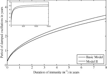
Period of damped oscillations as a function of duration of immunity $1/\alpha$. Figure insert: behaviour as $1/\alpha \to \infty$. All parameters are listed in Table 1.

3. The model with treatment

Various interventions can be adopted to slow the spread and lessen the impact of a disease. For a newly emerging virus, vaccines are unlikely to be available in the short term and the primary pharmaceutical intervention at the disposal of the health authorities is the use of antiviral drugs. A major concern with the widespread use of these drugs is the possibility of the emergence of a drug-resistant strain which is more virulent than the drug-sensitive strain. In this section, we consider the effects of treating symptomatically infected individuals with an antiviral drug. Asymptomatic individuals are not treated as there is no way of distinguishing them from the susceptible population. However, the preclinical cases, who proceed to the symptomatic state, can be treated once symptoms develop and they become visible to surveillance systems. We extend the basic model of Section 2 to describe two co-circulating strains, a drug-sensitive and drug-resistant strain. Treatment is given to individuals infected with either strain but only to clinical cases. An initially susceptible individual can get infected with either strain. However, once infected with the drug-sensitive strain, the treatment process may result in the emergence of the drug-resistant strain in said individual. As with the basic model, the subscripts ${}_A$ and ${}_S$ refer to asymptomatic and symptomatic individuals respectively. We further adopt the notation that subscripts ${}_r$ and ${}_{\mathit{tr}}$ refer to the drug-resistant strain and treated individuals respectively. Thus, we denote the disease compartments as follows:

• • $I_A$, infected with drug-sensitive strain and asymptomatic,
• • $I_S$, infected with drug-sensitive strain and symptomatic,
• • $I_{A\text{,}r}$, infected with drug-resistant strain and asymptomatic,
• • $I_{S\text{,}r}$, infected with drug-resistant strain and symptomatic,
• • $I_{S\text{,}\mathit{tr}}$, infected with drug-sensitive strain, symptomatic and receiving treatment,
• • $I_{S\text{,}r\text{,}\mathit{tr}}$, infected with drug-resistant strain, symptomatic and receiving treatment.

The transition diagram for the infection pathway is shown in Fig. 12 and the corresponding system of equations is

$$\frac{\mathit{dS}}{\mathit{dt}}=(\mu +\alpha )(1-S)-\alpha {\mathrm{\Sigma }}_I-({\beta }_A{I}_A+{\beta }_S{I}_S+{\beta }_{A\text{,}r}{I}_{A\text{,}r}+{\beta }_{S\text{,}r}{I}_{S\text{,}r}+\rho {\beta }_S{I}_{S\text{,}\mathit{tr}}+{\beta }_{S\text{,}r}{I}_{S\text{,}r\text{,}\mathit{tr}})S\text{,}$$ (14)

$$\frac{{\mathit{dI}}_A}{\mathit{dt}}=({\beta }_A{I}_A+{\beta }_S{I}_S+\rho {\beta }_S{I}_{S\text{,}\mathit{tr}})S-({\gamma }_A+\delta +\mu )I_A\text{,}$$ (15)

$$\frac{{\mathit{dI}}_S}{\mathit{dt}}=\delta I_A-({\gamma }_S+\theta +\mu )I_S\text{,}$$ (16)

$$\frac{{\mathit{dI}}_{A\text{,}r}}{\mathit{dt}}=({\beta }_{A\text{,}r}{I}_{A\text{,}r}+{\beta }_{S\text{,}r}{I}_{S\text{,}r}+{\beta }_{S\text{,}r}{I}_{S\text{,}r\text{,}\mathit{tr}})S-({\gamma }_A+{\delta }_r+\mu )I_{A\text{,}r}\text{,}$$ (17)

$$\frac{{\mathit{dI}}_{S\text{,}r}}{\mathit{dt}}={\delta }_r{I}_{A\text{,}r}-({\gamma }_S+\theta +\mu )I_{S\text{,}r}\text{,}$$ (18)

$$\frac{{\mathit{dI}}_{S\text{,}\mathit{tr}}}{\mathit{dt}}=-(r{\gamma }_S+q\eta +\mu )I_{S\text{,}\mathit{tr}}+\theta I_S\text{,}$$ (19)

$$\frac{{\mathit{dI}}_{S\text{,}r\text{,}\mathit{tr}}}{\mathit{dt}}=-({\gamma }_S+\mu )I_{S\text{,}r\text{,}\mathit{tr}}+q\eta I_{S\text{,}\mathit{tr}}+\theta I_{S\text{,}r}\text{,}$$ (20)

where ${\mathrm{\Sigma }}_I=I_A+I_S+I_{A\text{,}r}+I_{S\text{,}r}+I_{S\text{,}\mathit{tr}}+I_{S\text{,}r\text{,}\mathit{tr}}$. Each dependent variable represents the proportion of the total population that resides in that compartment. There is also an equation for the recovered compartment R. However, as before, adopting the constant population assumption ($\mathrm{\Lambda }=\mu N$) and noting that $R=1-(S+I_A+I_S+I_{A\text{,}r}+I_{S\text{,}r}+I_{S\text{,}\mathit{tr}}+I_{S\text{,}r\text{,}\mathit{tr}})$, we can discard this equation and limit our analysis to the above system. Symptomatic individuals are treated after $1/\theta$ days and, for the drug-sensitive strain alone, treatment is assumed to reduce the potential infectivity of such an individual by a factor $\rho$ and enable a faster recovery determined by r. We take $r>1$ so that individuals treated for the drug-sensitive strain recover faster than those treated for the drug-resistant strain. Following treatment for the drug-sensitive strain, the probability of the emergence of resistance is denoted by q with such resistance developing after an average of $1/\eta$ days. In addition, the transmission rates for the resistant strain are related via ${\beta }_{S\text{,}r}=c{\beta }_{A\text{,}r}$ with $c>1$. All other parameters are defined as before and are listed in Table 1.

Fig. 12.

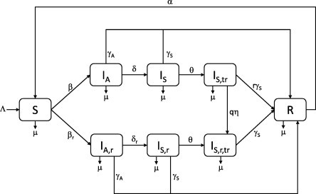
Transition diagram for the treatment model.

3.1. Basic reproduction number and equilibria

By inspection, it can be seen that the system (14), (15), (16), (17), (18), (19), (20) possesses a disease-free equilibrium, which we denote by $P^0$, and this can be used to calculate the basic reproduction number. The model consists of six diseased compartments, and we write the vectors $\tilde{\mathbf{F}}$ and $\tilde{\mathbf{V}}$ as

$$\tilde{\mathbf{F}}=\left[\begin{array}{c}\hfill ({\beta }_A{I}_A+{\beta }_S{I}_S+\rho {\beta }_S{I}_{S\text{,}\mathit{tr}})S\hfill \\ \hfill 0\hfill \\ \hfill ({\beta }_{A\text{,}r}{I}_{A\text{,}r}+{\beta }_{S\text{,}r}{I}_{S\text{,}r}+{\beta }_{S\text{,}r}{I}_{S\text{,}r\text{,}\mathit{tr}})S\hfill \\ \hfill 0\hfill \\ \hfill 0\hfill \\ \hfill 0\hfill \end{array}\right]\text{,}\tilde{\mathbf{V}}=\left[\begin{array}{c}\hfill ({\gamma }_A+\delta +\mu )I_A\hfill \\ \hfill -\delta I_A+({\gamma }_S+\theta +\mu )I_S\hfill \\ \hfill ({\gamma }_A+{\delta }_r+\mu )I_{A\text{,}r}\hfill \\ \hfill -{\delta }_r{I}_{A\text{,}r}+({\gamma }_S+\theta +\mu )I_{S\text{,}r}\hfill \\ \hfill (r{\gamma }_S+q\eta +\mu )I_{S\text{,}\mathit{tr}}-\theta I_S\hfill \\ \hfill ({\gamma }_S+\mu )I_{S\text{,}r\text{,}\mathit{tr}}-q\eta I_{S\text{,}\mathit{tr}}-\theta I_{S\text{,}r}\hfill \end{array}\right]\text{.}$$

The next generation matrix will then satisfy $K={\mathit{FV}}^{-1}$, where $F=\partial {\tilde{\mathbf{F}}}_i/\partial x_j{|}_{P^0}$ and $V=\partial {\tilde{\mathbf{V}}}_i/\partial x_j{|}_{P^0}$, and we find two nonzero eigenvalues given by

$$\begin{array}{cc}\hfill & R_1=R_A+R_S+R_T\text{,}\hfill \\ \hfill & R_2=R_{A\text{,}r}+R_{S\text{,}r}+R_{T\text{,}r}\text{,}\hfill \end{array}$$

where $R_A$ and $R_S$ are defined as for the basic model and

$$R_T=\frac{\rho {\beta }_S\delta \theta }{({\gamma }_A+\delta +\mu )({\gamma }_S+\theta +\mu )(r{\gamma }_S+q\eta +\mu )}\text{,}{R}_{A\text{,}r}=\frac{{\beta }_{A\text{,}r}}{{\gamma }_A+{\delta }_r+\mu }\text{,}$$

$$R_{S\text{,}r}=\frac{{\beta }_{S\text{,}r}{\delta }_r}{({\gamma }_S+\theta +\mu )({\gamma }_A+{\delta }_r+\mu )}\text{,}{R}_{T\text{,}r}=\frac{{\beta }_{S\text{,}r}\theta {\delta }_r}{({\gamma }_S+\theta +\mu )({\gamma }_A+{\delta }_r+\mu )({\gamma }_S+\mu )}\text{.}$$

We essentially get two reproduction numbers, one for each strain of the virus (drug-sensitive $R_1$ and drug-resistant $R_2$), and the basic reproduction number for the system will be the largest of these eigenvalues, $R_0=\max \{R_1\text{,}{R}_2\}$.

Setting the right-hand sides of Eqs. (14), (15), (16), (17), (18), (19), (20) equal to zero, we can determine the remaining equilibrium points. We find that another steady state $\widehat{P}=(\widehat{S}\text{,}0\text{,}0\text{,}{\hat{I}}_{A\text{,}r}\text{,}{\hat{I}}_{S\text{,}r}\text{,}0\text{,}{\hat{I}}_{S\text{,}r\text{,}\mathit{tr}})$ occurs where only the resistant strain is present. We obtain

$$\widehat{S}=\frac{1}{R_2}\text{,}$$ (21)

$${\hat{I}}_{A\text{,}r}=\frac{{\mathrm{\Omega }}_0{\mathrm{\Omega }}_2}{{\mathrm{\Omega }}_2{\mathrm{\Omega }}_3+\alpha ({\delta }_r+{\mathrm{\Omega }}_2)}\left(1-\frac{1}{R_2}\right)\text{,}$$ (22)

$${\hat{I}}_{S\text{,}r}=\frac{{\delta }_r{\mathrm{\Omega }}_0{\mathrm{\Omega }}_2}{{\mathrm{\Omega }}_2{\mathrm{\Omega }}_3{\mathrm{\Omega }}_5+\alpha {\mathrm{\Omega }}_5({\delta }_r+{\mathrm{\Omega }}_2)}\left(1-\frac{1}{R_2}\right)\text{,}$$ (23)

$${\hat{I}}_{S\text{,}r\text{,}\mathit{tr}}=\frac{{\delta }_r\theta {\mathrm{\Omega }}_0}{{\mathrm{\Omega }}_2{\mathrm{\Omega }}_3{\mathrm{\Omega }}_5+\alpha {\mathrm{\Omega }}_5({\delta }_r+{\mathrm{\Omega }}_2)}\left(1-\frac{1}{R_2}\right)\text{,}$$ (24)

where, for convenience, we have set

$$\begin{array}{cc}\hfill & {\mathrm{\Omega }}_3={\gamma }_A+{\delta }_r+\mu \text{,}\hfill \\ \hfill & {\mathrm{\Omega }}_4=r{\gamma }_S+q\eta +\mu \text{,}\hfill \\ \hfill & {\mathrm{\Omega }}_5={\gamma }_S+\theta +\mu \text{,}\hfill \end{array}$$

and ${\mathrm{\Omega }}_0\text{,}{\mathrm{\Omega }}_1$ and ${\mathrm{\Omega }}_2$ are defined as before. Clearly, when $R_2=1$ we simply get the disease-free equilibrium with $\widehat{P}=P^0$. When $R_2<1$ the infected populations become negative, which is not a biologically feasible solution. Hence, $\widehat{P}$ only exists when $R_2>1$. Finally, a third equilibrium state can also be achieved where both drug-sensitive and drug-resistant strains coexist. We denote this equilibrium by $P^{\ast }$ and find

$$S^{\ast }=\frac{1}{R_1}\text{,}$$ (25)

$$I_A^{\ast }=\frac{{\mathrm{\Omega }}_0{\mathrm{\Omega }}_2{\mathrm{\Omega }}_3{\mathrm{\Omega }}_4{\mathrm{\Omega }}_5(R_1-R_2)}{{\mathrm{\Omega }}_2{\mathrm{\Omega }}_3(R_1-R_2){\mathrm{\Pi }}_0+{\mathrm{\Pi }}_1}\left(1-\frac{1}{R_1}\right)\text{,}$$ (26)

$$I_S^{\ast }=\frac{\delta {\mathrm{\Omega }}_0{\mathrm{\Omega }}_2{\mathrm{\Omega }}_3{\mathrm{\Omega }}_4(R_1-R_2)}{{\mathrm{\Omega }}_2{\mathrm{\Omega }}_3(R_1-R_2){\mathrm{\Pi }}_0+{\mathrm{\Pi }}_1}\left(1-\frac{1}{R_1}\right)\text{,}$$ (27)

$$I_{A\text{,}r}^{\ast }=\frac{{\beta }_{S\text{,}r}\delta q\eta \theta {\mathrm{\Omega }}_0{\mathrm{\Omega }}_5}{{\mathrm{\Omega }}_2{\mathrm{\Omega }}_3{\mathrm{\Omega }}_5(R_1-R_2){\mathrm{\Pi }}_0+{\mathrm{\Omega }}_5{\mathrm{\Pi }}_1}\left(1-\frac{1}{R_1}\right)\text{,}$$ (28)

$$I_{S\text{,}r}^{\ast }=\frac{{\delta }_r{\beta }_{S\text{,}r}\delta q\eta \theta {\mathrm{\Omega }}_0}{{\mathrm{\Omega }}_2{\mathrm{\Omega }}_3{\mathrm{\Omega }}_5(R_1-R_2){\mathrm{\Pi }}_0+{\mathrm{\Omega }}_5{\mathrm{\Pi }}_1}\left(1-\frac{1}{R_1}\right)\text{,}$$ (29)

$$I_{S\text{,}\mathit{tr}}^{\ast }=\frac{\delta \theta {\mathrm{\Omega }}_0{\mathrm{\Omega }}_2{\mathrm{\Omega }}_3(R_1-R_2)}{{\mathrm{\Omega }}_2{\mathrm{\Omega }}_3(R_1-R_2){\mathrm{\Pi }}_0+{\mathrm{\Pi }}_1}\left(1-\frac{1}{R_1}\right)\text{,}$$ (30)

$$I_{S\text{,}r\text{,}\mathit{tr}}^{\ast }=\frac{q\eta \delta \theta {\mathrm{\Omega }}_0[{\mathrm{\Omega }}_2{\mathrm{\Omega }}_3{\mathrm{\Omega }}_5(R_1-R_2)+\theta {\delta }_r{\beta }_{S\text{,}r}]}{{\mathrm{\Omega }}_2^2{\mathrm{\Omega }}_3{\mathrm{\Omega }}_5(R_1-R_2){\mathrm{\Pi }}_0+{\mathrm{\Omega }}_2{\mathrm{\Omega }}_5{\mathrm{\Pi }}_1}\left(1-\frac{1}{R_1}\right)\text{,}$$ (31)

and where, for convenience, we define

$${\mathrm{\Pi }}_0={\mathrm{\Omega }}_1{\mathrm{\Omega }}_4{\mathrm{\Omega }}_5+\alpha ({\mathrm{\Omega }}_4{\mathrm{\Omega }}_5+{\mathrm{\Omega }}_4\delta +\theta \delta )\text{,}$$

$${\mathrm{\Pi }}_1=\frac{\theta q\eta \delta }{{\mathrm{\Omega }}_2}[{\beta }_{S\text{,}r}(\alpha {\mathrm{\Omega }}_2+{\mathrm{\Omega }}_2{\mathrm{\Omega }}_3+\alpha {\delta }_r)+\alpha {\mathrm{\Omega }}_2{\mathrm{\Omega }}_3(R_1-R_2)]\text{.}$$

When $R_1=1$ we simply have the disease-free equilibrium with $P^{\ast }=P^0$. When $R_1<1$ we find that $S^{\ast }>1$ which is not biologically feasible. So we require $R_1>1$. In addition, if we consider the expression for $I_{A\text{,}r}^{\ast }$ we see that the denominator must be positive to ensure $I_{A\text{,}r}⩾0$. Thus we require

$${\mathrm{\Omega }}_2{\mathrm{\Omega }}_3(R_1-R_2){\mathrm{\Pi }}_0+{\mathrm{\Pi }}_1>0\text{.}$$ (32)

Now, considering the expression for $I_A^{\ast }$ we see that the numerator must also be positive which requires $R_1>R_2$ and thus (32) is automatically satisfied. The above results on the existence of the equilibria are summarised in Theorem 4. The theorem is expressed graphically in Fig. 13 , where the existence of $P^0\text{,}\widehat{P}$ and $P^{\ast }$ is shown in $R_1-R_2$ parameter space.

Theorem 1

The system (14), (15), (16), (17), (18), (19), (20) always has a disease-free equilibrium $P^0$ . An endemic equilibrium $\widehat{P}$ , given by (21), (22), (23), (24) and where only the drug-resistant strain is present in the population, exists when $R_2>1$ . Another endemic equilibrium $P^{\ast }$ , given by (25), (26), (27), (28), (29), (30), (31) and where both drug-sensitive and drug-resistant strains are present, exists when $R_1>1$ and $R_1>R_2$.

Fig. 13.

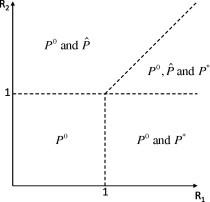
Existence of equilibria in $R_1-R_2$ parameter space. $P^0$ denotes the disease-free state, $\widehat{P}$ denotes the presence of only the drug-resistant strain and $P^{\ast }$ denotes the coexistence of both drug-sensitive and drug-resistant strains.

3.2. Local stability analysis

In this section we consider the local stability properties of the three equilibria.

Theorem 2

The disease-free equilibrium $P^0$ of the system (14), (15), (16), (17), (18), (19), (20) is locally asymptotically stable when $R_2<1$ and $R_1<1$ .

Proof

The characteristic equation, determined form the Jacobian matrix evaluated at $P^0$, is a seventh order polynomial which we can write in the form

$$(\lambda +{\mathrm{\Omega }}_0)G(\lambda )F(\lambda )=(\lambda +{\mathrm{\Omega }}_0){\displaystyle \sum _{i=0}^3}{g}_i{\lambda }^i{\displaystyle \sum _{j=0}^3}{f}_j{\lambda }^j\text{,}$$

where the cubic coefficients are given by

$$g_2={\mathrm{\Omega }}_2+{\mathrm{\Omega }}_3+{\mathrm{\Omega }}_5-{\beta }_{A\text{,}r}\text{,}$$

$$g_1=({\mathrm{\Omega }}_3-{\beta }_{A\text{,}r})({\mathrm{\Omega }}_2+{\mathrm{\Omega }}_5)+{\mathrm{\Omega }}_2{\mathrm{\Omega }}_5-{\delta }_r{\beta }_{S\text{,}r}\text{,}$$

$$g_0={\mathrm{\Omega }}_2{\mathrm{\Omega }}_3{\mathrm{\Omega }}_5(1-R_2)\text{,}$$

$$f_2={\mathrm{\Omega }}_1+{\mathrm{\Omega }}_4+{\mathrm{\Omega }}_5-{\beta }_A\text{,}$$

$$f_1=({\mathrm{\Omega }}_1-{\beta }_A)({\mathrm{\Omega }}_4+{\mathrm{\Omega }}_5)+{\mathrm{\Omega }}_4{\mathrm{\Omega }}_5-\delta {\beta }_S\text{,}$$

$$f_0={\mathrm{\Omega }}_1{\mathrm{\Omega }}_4{\mathrm{\Omega }}_5(1-R_1)\text{.}$$

The disease-free equilibrium will be locally asymptotically stable when all eigenvalues ${\lambda }_i$ have negative real part. The eigenvalue ${\lambda }_1=-{\mathrm{\Omega }}_0<0$ is easily obtained. All roots of the polynomial $G=0$ will have negative real part when

$$g_0>0\text{,}{g}_2>0\text{,}{g}_1{g}_2-g_0>0\text{.}$$

The first inequality can only be satisfied when $R_2<1$. The second inequality can be written in the form

$$R_2<1+\frac{{\mathrm{\Omega }}_2{\mathrm{\Omega }}_5({\mathrm{\Omega }}_2+{\mathrm{\Omega }}_5)+c{\delta }_r({\mathrm{\Omega }}_2+\theta )({\mathrm{\Omega }}_2+{\mathrm{\Omega }}_3+{\mathrm{\Omega }}_5)}{{\mathrm{\Omega }}_2{\mathrm{\Omega }}_3{\mathrm{\Omega }}_5}\text{,}$$

which is automatically satisfied when $R_2<1$. Finally, the third inequality can be written as

$$g_1{g}_2-g_0=\frac{1}{{\mathrm{\Omega }}_2{\mathrm{\Omega }}_5}\left[{\mathrm{\Omega }}_3{\beta }_{S\text{,}r}{\delta }_r(1-R_2)({\mathrm{\Omega }}_2+{\mathrm{\Omega }}_5)({\mathrm{\Omega }}_2+\theta )+g_2{\mathrm{\Omega }}_2{\beta }_{S\text{,}r}{\delta }_r({\mathrm{\Omega }}_2+\theta )+g_2{\mathrm{\Omega }}_5{\beta }_{S\text{,}r}{\delta }_r\theta g_2{\mathrm{\Omega }}_2^2{\mathrm{\Omega }}_5^2+{\mathrm{\Omega }}_2{\mathrm{\Omega }}_3^2{\mathrm{\Omega }}_5(1-R_2{)}^2({\mathrm{\Omega }}_2+{\mathrm{\Omega }}_5)+{\mathrm{\Omega }}_2{\mathrm{\Omega }}_3{\mathrm{\Omega }}_5(1-R_2)({\mathrm{\Omega }}_2^2+{\mathrm{\Omega }}_2{\mathrm{\Omega }}_5+{\mathrm{\Omega }}_5^2)\right]>0\text{.}$$

Thus, all roots of the cubic $G=0$ will have negative real part when $R_2<1$. Similarly, the roots of the polynomial $F=0$ will have negative real part when

$$f_0>0\text{,}{f}_2>0\text{,}{f}_1{f}_2-f_0>0\text{.}$$

The first inequality is satisfied only when $R_1<1$. The second inequality can be written in the form

$$R_1<1+\frac{c\delta ({\mathrm{\Omega }}_1+{\mathrm{\Omega }}_4+{\mathrm{\Omega }}_5)({\mathrm{\Omega }}_4+\rho \theta )+{\mathrm{\Omega }}_4{\mathrm{\Omega }}_5({\mathrm{\Omega }}_4+{\mathrm{\Omega }}_5)}{{\mathrm{\Omega }}_1{\mathrm{\Omega }}_4{\mathrm{\Omega }}_5}\text{,}$$

which is automatically satisfied when $R_1<1$ and, finally, the third inequality can be written as

$$f_1{f}_2-f_0={\mathrm{\Omega }}_1(1-R_1)\left[{\mathrm{\Omega }}_1({\mathrm{\Omega }}_4+{\mathrm{\Omega }}_5)(1-R_1)+{\mathrm{\Omega }}_5^2+{\mathrm{\Omega }}_4{\mathrm{\Omega }}_5+{\mathrm{\Omega }}_4^2+({\mathrm{\Omega }}_4+{\mathrm{\Omega }}_5)\left(\frac{{\beta }_S\delta }{{\mathrm{\Omega }}_5}+\frac{\rho {\beta }_S\delta \theta }{{\mathrm{\Omega }}_4{\mathrm{\Omega }}_5}\right)\right]+\frac{f_2\rho {\beta }_S\delta \theta }{{\mathrm{\Omega }}_4}+\frac{f_2{\beta }_S\delta {\mathrm{\Omega }}_4}{{\mathrm{\Omega }}_5}+\frac{f_2\rho {\beta }_S\delta \theta }{{\mathrm{\Omega }}_5}+f_2{\mathrm{\Omega }}_4{\mathrm{\Omega }}_5>0\text{.}$$

Thus, the all roots of cubic $F=0$ have negative real part when $R_1<1$. □

Analytical results for the local stability properties of the endemic equilibria are not easily obtained due to the complicated algebraic nature of the characteristic equations. For the drug-resistant equilibrium $\widehat{P}$ the characteristic equation is

$$H(\lambda )L(\lambda )={\displaystyle \sum _{i=0}^3}{h}_i{\lambda }^i{\displaystyle \sum _{j=0}^4}{l}_j{\lambda }^j\text{,}$$

with coefficients

$$h_3=R_2\text{,}$$

$$h_2=R_2({\mathrm{\Omega }}_1+{\mathrm{\Omega }}_4+{\mathrm{\Omega }}_5)-{\beta }_A\text{,}$$

$$h_1=R_2({\mathrm{\Omega }}_1{\mathrm{\Omega }}_5+{\mathrm{\Omega }}_1{\mathrm{\Omega }}_4+{\mathrm{\Omega }}_4{\mathrm{\Omega }}_5)-{\beta }_A({\mathrm{\Omega }}_4+{\mathrm{\Omega }}_5)-\delta {\beta }_S\text{,}$$

$$h_0={\mathrm{\Omega }}_1{\mathrm{\Omega }}_4{\mathrm{\Omega }}_5(R_2-R_1)\text{,}$$

$$l_4=\mathrm{\Gamma }{R}_2\text{,}$$

$$l_3={\mathrm{\Omega }}_0{\mathrm{\Omega }}_2{\mathrm{\Omega }}_3{R}_2(R_2-1)+\mathrm{\Gamma }{R}_2({\mathrm{\Omega }}_0+{\mathrm{\Omega }}_2+{\mathrm{\Omega }}_3+{\mathrm{\Omega }}_5)-\mathrm{\Gamma }{\beta }_{A\text{,}r}\text{,}$$

$$l_2={\mathrm{\Omega }}_0{\mathrm{\Omega }}_2{\mathrm{\Omega }}_3{R}_2(R_2-1)({\mathrm{\Omega }}_2+{\mathrm{\Omega }}_3+{\mathrm{\Omega }}_5+\alpha )+\mathrm{\Gamma }{R}_2({\mathrm{\Omega }}_0{\mathrm{\Omega }}_2+{\mathrm{\Omega }}_0{\mathrm{\Omega }}_5+{\mathrm{\Omega }}_2{\mathrm{\Omega }}_5+{\mathrm{\Omega }}_2{\mathrm{\Omega }}_3+{\mathrm{\Omega }}_0{\mathrm{\Omega }}_3+{\mathrm{\Omega }}_3{\mathrm{\Omega }}_5)-\mathrm{\Gamma }{\beta }_{A\text{,}r}({\mathrm{\Omega }}_0+{\mathrm{\Omega }}_2+{\mathrm{\Omega }}_5)-\mathrm{\Gamma }{\beta }_{S\text{,}r}{\delta }_r\text{,}$$

$$l_1={\mathrm{\Omega }}_0{\mathrm{\Omega }}_2{\mathrm{\Omega }}_3{R}_2(R_2-1)(\alpha +{\mathrm{\Omega }}_2{\mathrm{\Omega }}_5+\alpha {\mathrm{\Omega }}_5+{\mathrm{\Omega }}_3{\mathrm{\Omega }}_5)+\mathrm{\Gamma }{R}_2({\mathrm{\Omega }}_0{\mathrm{\Omega }}_2{\mathrm{\Omega }}_5+{\mathrm{\Omega }}_0{\mathrm{\Omega }}_2{\mathrm{\Omega }}_3+{\mathrm{\Omega }}_2{\mathrm{\Omega }}_3{\mathrm{\Omega }}_5+{\mathrm{\Omega }}_0{\mathrm{\Omega }}_3{\mathrm{\Omega }}_5)-\mathrm{\Gamma }{\mathrm{\Omega }}_2{\mathrm{\Omega }}_3{\mathrm{\Omega }}_5{R}_2-{\mathrm{\Omega }}_0\mathrm{\Gamma }{\beta }_{A\text{,}r}({\mathrm{\Omega }}_2+{\mathrm{\Omega }}_5)-{\mathrm{\Omega }}_0\mathrm{\Gamma }{\delta }_r{\beta }_{S\text{,}r}\text{,}$$

$$l_0={\mathrm{\Omega }}_0{\mathrm{\Omega }}_2{\mathrm{\Omega }}_3{R}_2(R_2-1)({\delta }_r\theta \alpha +{\mathrm{\Omega }}_2{\mathrm{\Omega }}_3{\mathrm{\Omega }}_5+{\mathrm{\Omega }}_2{\delta }_r\alpha +\alpha {\mathrm{\Omega }}_2{\mathrm{\Omega }}_5)\text{.}$$

where $\mathrm{\Gamma }={\mathrm{\Omega }}_2{\mathrm{\Omega }}_3+\alpha ({\delta }_r+{\mathrm{\Omega }}_2)$.

The conditions for $H=0$ to have roots with negative real part are

$$(\text{i})h_0>0\text{,}(\text{ii})h_2>0\text{,}(\text{iii})h_1{h}_2-h_0{h}_3>0\text{,}$$

which can be written as

$$(\text{i})R_2>R_1\text{,}$$

$$(\text{ii})R_2>\mathrm{\Phi }{R}_1\text{,}$$

$$(\text{iii}){\mathrm{\Omega }}_1(R_2-R_1)\left[{\mathrm{\Omega }}_1({\mathrm{\Omega }}_4+{\mathrm{\Omega }}_5)(R_2-R_1)+R_2({\mathrm{\Omega }}_4^2+{\mathrm{\Omega }}_4{\mathrm{\Omega }}_5+{\mathrm{\Omega }}_5^2)+\frac{{\beta }_S\delta ({\mathrm{\Omega }}_4+{\mathrm{\Omega }}_5)({\mathrm{\Omega }}_4+\rho \theta )}{{\mathrm{\Omega }}_4{\mathrm{\Omega }}_5}\right]+{\mathrm{\Omega }}_4{\mathrm{\Omega }}_5{h}_2{R}_2+h_2\left(\frac{{\beta }_S\delta {\mathrm{\Omega }}_4}{{\mathrm{\Omega }}_5}+\frac{\rho {\beta }_S\delta \theta }{{\mathrm{\Omega }}_4}+\frac{\rho {\beta }_S\delta \theta }{{\mathrm{\Omega }}_5}\right)>0\text{,}$$

where

$$\mathrm{\Phi }=\frac{{\mathrm{\Omega }}_1{\mathrm{\Omega }}_4{\mathrm{\Omega }}_5}{({\mathrm{\Omega }}_1+{\mathrm{\Omega }}_4+{\mathrm{\Omega }}_5)[{\mathrm{\Omega }}_4{\mathrm{\Omega }}_5+c\delta ({\mathrm{\Omega }}_4+\rho \theta )]}\text{.}$$

Since $0<\mathrm{\Phi }<1$, all inequalities are satisfied when $R_2>R_1$. The conditions for $L=0$ to have roots with negative real part are

$$(\text{i})l_0>0\text{,}(\text{ii})l_3>0\text{,}(\text{iii})L_1(R_2)=l_2{l}_3-l_1{l}_4>0\text{,}(\text{iv})L_2(R_2)=l_1(l_2{l}_3-l_1{l}_4)-l_0{l}_3^2>0\text{.}$$

It can be easily shown analytically that (i) and (ii) are always satisfied when $R_2>1$. The other conditions are not so readily analysed and we provide a numerical analysis for the specific case of an influenza virus. Currently, the most widely used antiviral drugs are the neuraminidase inhibitors oseltamivir and zanamivir. The emergence of resistance to oseltamivir was documented during the 2009 H1N1 pandemic, however, little zanamivir-resistant cases were detected [41], [43]. All relevant parameter values for influenza are listed in Table 1. We plot conditions (iii) and (iv) in Fig. 14 and it is clear that both inequalities are satisfied for all $R_2$. Thus, we conclude that, for the case of influenza, $\widehat{P}$ is locally stable when $R_2>R_1$.

Fig. 14.

Behaviour of the functions $L_1(R_2)$ and $L_2(R_2)$ for positive $R_2$.

The characteristic equation corresponding to the endemic equilibrium $P^{\ast }$ is intractable to an analytical analysis. However, based on previous results, we would expect this fixed point to be locally stable for all $R_1>1$ and $R_2<R_1$. To analyse the stability properties we generate a mesh in $R_1-R_2$ parameter space and then at each point we numerically determine the local stability of each equilibrium through examination of the eigenvalues of the Jacobian matrix. We indicate stability of $P^0\text{,}\widehat{P}$ and $P^{\ast }$ with a cross, circle and triangle respectively and the results are displayed in Fig. 15, Fig. 16 .

Fig. 15.

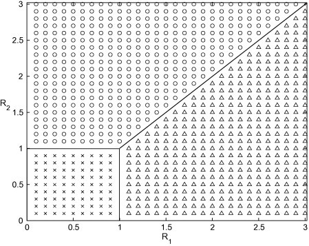
Stability properties determined from eigenvalues of the Jacobian matrix. Crosses indicated points where $P^0$ is stable, circles indicate points where $\widehat{P}$ is stable and triangles indicate points where $P^{\ast }$ is stable. Parameter values are listed in Table 1.

Fig. 16.

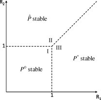
Stability of equilibria in $R_1-R_2$ parameter space. $P^0$ denotes the disease-free state, $\widehat{P}$ denotes the presence of only the drug-resistant strain and $P^{\ast }$ denotes the coexistence of both drug-sensitive and drug-resistant strains.

It can be seen that there are three distinct regions: region I where the disease-free equilibrium $P^0$ is stable, region II where $\widehat{P}$ is stable and only the drug-resistant strain of the virus is present and region III where $P^{\ast }$ is stable and both the drug-sensitive and drug-resistant strains of the virus coexist. Similar results have been documented for models of tuberculosis treatment when the latent state is considered [44], [45], [46] in place of an asymptomatic infectious state, which can account for approximately one third of all influenza infections.

In Fig. 17 (a) we show a solution corresponding to region I. Here the disease-free equilibrium is stable and, following a short initial increase, the virus dies out rapidly. In Fig. 17(b) we show a solution corresponding to region II. The solution initially oscillates around the fixed point $\widehat{P}$ and approaches it as $t\to \infty$. In Fig. 17(c) we show a solution corresponding to region III. Again, after some initial oscillatory behaviour the solution approaches $P^{\ast }$. Finally, for completeness, we also consider the upper portion of region III where both endemic equilibria exist (see Fig. 13). A solution corresponding to this region is shown in Fig. 17(d). Both endemic equilibria exist and the solution approaches the stable equilibrium $P^{\ast }$.

Fig. 17.

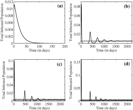
Solution of the treatment model with initial conditions $S(0)=0.99$, $I_S(0)=0.01$ and $I_A(0)=I_{A\text{,}r}(0)=I_{S\text{,}r}(0)=I_{S\text{,}\mathit{tr}}(0)=I_{S\text{,}r\text{,}\mathit{tr}}(0)=0$. Circles and triangles indicate the locations of $\widehat{P}$ and $P^{\ast }$ respectively. All parameters are listed in Table 1. (a) $R_1=0.9$, $R_2=0.8$, (b) $R_1=1.6$, $R_2=1.8$, (c) $R_1=1.7$, $R_2=0.8$, and (d) $R_1=2.1$, $R_2=1.1$.

When a novel influenza virus emerges, the delay in delivering a strain-specific vaccine requires preparedness plans to reply on other containment strategies. The sole pharmaceutical measure available to public health authorities to alleviate the pandemic impact is the use of antiviral drugs for therapeutic or prophylactic use. It is possible that health systems would have to reply on these drugs for several months while a vaccine is developed and, thus, their timely availability in sufficient quantities to meet international requirements would be crucial. Such a demand could only be met if the drugs were stockpiled in advance of a pandemic [47], [48]. If a highly virulent drug-resistant strain were to emerge the economic impact of losing valuable stockpiles would further devastate already overburdened health systems. Therefore, understanding the dynamics of the emergence of drug resistance is an important topic in the preparation for future pandemic outbreaks. It has been shown that widespread use of antiviral drugs should be avoided during a pandemic, except in the case of high reproduction number, to prevent a more virulent drug-resistant strain developing [49]. This theory is supported by our findings. The existence and stability of the two strains are completely determined by the values of the reproduction numbers $R_1$ and $R_2$. The greater the reproduction number of the drug-sensitive strain the greater the reproduction number required by the drug-resistant strain to become endemic in the population. If the reproduction number of the sensitive strain is close to 1 then a lower value of $R_2$ can allow the drug-resistant strain to become endemic.

4. Discussion

A mathematical elaboration of some dynamic features of an epidemiological model that explicitly considers asymptomatic infectious cases and loss of immunity, together with the associated model that accounts for treatment and the development of drug resistance was presented in this paper. It was shown that the dynamics of the simple model without intervention are entirely determined by the basic reproduction number $R_0$, with the disease becoming endemic when $R_0>1$ and dying out when $R_0<1$. In addition, it was demonstrated that the long-term dynamics are characterised by damped oscillations approaching an endemic state, whose period of oscillation is greatly influenced by the rate at which infection acquired immunity is lost. A comparison was provided between this model and another commonly used model in which the preclinical infectious state is absent. It was shown that, for the general model, two unique transmission rates are obtained. For the specific case of influenza the transmission rates are equal, however, the models still predict quantitatively different disease incidence. By considering a simple public health intervention, where the easily identifiable symptomatic cases are isolated from the general population, it was shown that, under certain conditions, neglecting the preclinical state could underestimate the peak incidence and the resultant burden on public health systems during an epidemic. Better estimates for the duration of preclinical viral shedding could help to provide more accurate estimates for the impact of pre-symptomatic influenza transmission. We emphasis that the two models considered here cannot be directly compared and we merely present the two approaches and highlight their similarities and differences.

An interesting result could also be derived from this analysis regarding the stability of the model when treatment and the development of drug resistance are considered. In addition to the locally stable disease free equilibrium, two other endemic equilibria were identified. The first corresponds to the presence of the resistant strain when $R_2>1$ and, for influenza parameter values, is locally stable when $R_2>R_1$. The second corresponds to the co-circulation of both the drug-sensitive and resistant strains when $R_1>1$ and $R_2<R_1$. Elaboration of the second endemic equilibrium is mathematically intractable. However, a graphical analysis of the stability properties, in the case of influenza, indicates that it is always locally stable. We note, however, that the effects of back-mutation from resistant to sensitive strains was neglected. This might possibly occur when the resistant strain carries a cost and is the reason underlying the fact that there is an equilibrium where only the resistant strain is present and no equilibrium with only the sensitive strain.

References

- 1.Fraser C., Riley S., Anderson R.M., Ferguson N.M. Factors that make an infectious disease outbreak controllable. PNAS. 2004;101:6146. doi: 10.1073/pnas.0307506101. [DOI] [PMC free article] [PubMed] [Google Scholar]
- 2.Mathews J.D., McCaw C.T., McVernon J., McBryde E.S., McCaw J.M. A biological model for influenza transmission: pandemic planning implications of asymptomatic infection and immunity. PLoS ONE. 2007;2:e1220. doi: 10.1371/journal.pone.0001220. [DOI] [PMC free article] [PubMed] [Google Scholar]
- 3.Kelly H.A., Priest P.C., Mercer G.N., Dowse G.K. We should not be complacent about our population-based public health response to the first influenza pandemic of the century. BMC Public Health. 2011;11:78. doi: 10.1186/1471-2458-11-78. [DOI] [PMC free article] [PubMed] [Google Scholar]
- 4.Longini I.M., Halloran M.E., Nizam A., Yang Y. Containing pandemic influenza with antiviral agents. Am. J. Epidemiol. 2004;159:623. doi: 10.1093/aje/kwh092. [DOI] [PubMed] [Google Scholar]
- 5.Arino J., Brauer F., van den Driessche P., Watmough J., Wu J. A model for influenza vaccination and antiviral treatment. J. Theor. Biol. 2008;253:118. doi: 10.1016/j.jtbi.2008.02.026. [DOI] [PubMed] [Google Scholar]
- 6.McCaw J.M., Wood L.G., McCaw C.T., McVernon J. Impact of emerging antiviral drug resistance on influenza containment and spread: influence of subclinical infection and strategic use of a stockpile containing one or two drugs. PLoS ONE. 2008;3:e2362. doi: 10.1371/journal.pone.0002362. [DOI] [PMC free article] [PubMed] [Google Scholar]
- 7.Stilianakis N.I., Perelson A.S., Hayden F.G. Emergence of drug resistance during an influenza epidemic: insights from a mathematical model. J. Infect. Dis. 1998;177:863. doi: 10.1086/515246. [DOI] [PubMed] [Google Scholar]
- 8.Regoes R.R., Bonhoeffer S. Emergence of drug-resistant influenza virus: population dynamical considerations. Science. 2006;312:380. doi: 10.1126/science.1122947. [DOI] [PubMed] [Google Scholar]
- 9.Débarre F., Bonhoeffer S., Regoes R.R. The effect of population structure on the emergence of drug resistance during influenza pandemics. J.R. Soc. Interface. 2007;4:893. doi: 10.1098/rsif.2007.1126. [DOI] [PMC free article] [PubMed] [Google Scholar]
- 10.Wu J.T., Riley S., Fraser C., Leung G.M. Reducing the impact of the next influenza pandemic using household-based public health interventions. PLoS Med. 2006;3:1532. doi: 10.1371/journal.pmed.0030361. [DOI] [PMC free article] [PubMed] [Google Scholar]
- 11.Moghadas S.M., Bowman C.S., Röst G., Wu J. Population-wide emergence of antiviral resistance during pandemic influenza. PLoS ONE. 2008;3:e1839. doi: 10.1371/journal.pone.0001839. [DOI] [PMC free article] [PubMed] [Google Scholar]
- 12.Alexander M.E., Bowman C.S., Feng Z., Gardam M., Moghadas S.M., Röst G., Wu J., Yan P. Emergence of drug resistance: implications for antiviral control of pandemic influenza. Proc. R. Soc. B. 2007;274:1675. doi: 10.1098/rspb.2007.0422. [DOI] [PMC free article] [PubMed] [Google Scholar]
- 13.Keeling M., Rohani P. Princeton University Press; 2008. Modelling Infectious Diseases in Humans and Animals. [Google Scholar]
- 14.Kemper J.T. The effects of asymptomatic attacks on the spread of infectious disease: a deterministic model. Bull. Math. Biol. 1978;40:707. doi: 10.1007/BF02460601. [DOI] [PubMed] [Google Scholar]
- 15.Anderson R.M., May R.M. Oxford University Press; 1991. Infectious Diseases of Humans: Dynamics and Control. [Google Scholar]
- 16.van den Driessche P., Watmough J. Mathematical Epidemiology. Springer; New York: 2008. Further notes on the basic reproductive number; p. 159. [Google Scholar]
- 17.van den Driessche P., Watmough J. Reproduction numbers and sub-threshold endemic equilibria for compartmental models of disease transmission. Math. BioSci. 2001;180:29. doi: 10.1016/s0025-5564(02)00108-6. [DOI] [PubMed] [Google Scholar]
- 18.Diekmann O., Heesterbeek J.A.P. Wiley; Chichester, UK: 2000. Mathematical Epidemiology of Infectious Diseases: Model Building, Analysis and Interpretation. [Google Scholar]
- 19.Diekmann O., Heesterbeek J.A.P., Roberts M.G. The construction of next-generation matrices for compartmental epidemic models. J. R. Soc. Interface. 2010;7:873. doi: 10.1098/rsif.2009.0386. [DOI] [PMC free article] [PubMed] [Google Scholar]
- 20.Gu Y., Komiya N., Kamiya H., Yasuo Y., Taniguchi K., Okabe N. Pandemic (H1N1) 2009 transmission during presymptomatic phase, Japan. Emerg. Infect. Dis. 2011;17:1737. doi: 10.3201/eid1709.101411. [DOI] [PMC free article] [PubMed] [Google Scholar]
- 21.P. Marquez, D. Tereshita, L. Engish, Pre-symptomatic health care worker transmission of pandemic (H1N1) 2009 influenza in acute care settings, Acute Communicable Disease Control Program, Los Angeles, California, Special Studies Report, 2009, Los Angeles County Department of Public Health. <http://www.ph.lacounty.gov/acd/reports/annual/2009SpecialStudies.pdf>.
- 22.Lau L.H.L., Cowling B.J., Fang V.J., Chan K.H., Lau E.H.Y., Lipsitch M., Cheng C.K.Y., Nouck P.M., Uyeki T.M., Peiris J.S.M., Leung G.M. Viral shedding and clinical illness in naturally acquired influenza virus infections. J. Infect. Dis. 2010;201:1509. doi: 10.1086/652241. [DOI] [PMC free article] [PubMed] [Google Scholar]
- 23.Sheat K. An investigation into an explosive outbreak of influenza – New Plymouth. Commun. Dis. N. Z. 1992;92:18. [Google Scholar]
- 24.Webb G.F., Hsieh Y.-H., Wu J., Blaser M.J. Pre-symptomatic influenza transmission surveillance and school closings: implications for novel influenza A (H1N1) Math. Model. Nat. Phenom. 2010;5:191. [Google Scholar]
- 25.World Health Organisation Writing Group Nonpharmaceutical interventions for pandemic influenza, international measures. Emerg. Infect. Dis. 2006;12:81. doi: 10.3201/eid1201.051370. [DOI] [PMC free article] [PubMed] [Google Scholar]
- 26.Ferguson N.M., Mallett S., Jackson H., Roberts N., Ward P. A population-dynamic model for evaluating the potential spread of resistant influenza virus infections during community-based use of antivirals. J. Antimicrob. Chemother. 2003;51:977. doi: 10.1093/jac/dkg136. [DOI] [PubMed] [Google Scholar]
- 27.Patrozou E., Mermel L.A. Does infuenza transmission occur from asymptomatic infection or prior to symptom onset? Public Health Rep. 2009;124:193. doi: 10.1177/003335490912400205. [DOI] [PMC free article] [PubMed] [Google Scholar]
- 28.Donnelly C.A., Finelli L., Cauchemez S. Serial intervals and the temporal distribution of secondary infections within households of 2009 pandemic influenza A (H1N1): implications for influenza control recommendations. Clin. Infect. Dis. 2011;52(S1):S123. doi: 10.1093/cid/ciq028. [DOI] [PMC free article] [PubMed] [Google Scholar]
- 29.Elvebeack L.R., Fox J.P., Ackerman E., Langworthy A., Boyd M., Gatewood L. An influenza simulation model for immunization studies. Am. J. Epidemiol. 1976;103:152. doi: 10.1093/oxfordjournals.aje.a112213. [DOI] [PubMed] [Google Scholar]
- 30.Carrat F., Vergu E., Ferguson N.M., Lemaitre M., Cauchemez S., Leach S., Valleron A.J. Time lines of infection and disease in human influenza: a review of volunteer challenge studies. Am. J. Epidemiol. 2008;167:775. doi: 10.1093/aje/kwm375. [DOI] [PubMed] [Google Scholar]
- 31.Ghani A.C., Baguelin M., Griffin J. The early transmission dynamics of H1N1pdm influenza in the United Kingdom. PLoS Curr. Influenza. 2009:RRN1130. doi: 10.1371/currents.RRN1130. [DOI] [PMC free article] [PubMed] [Google Scholar]
- 32.Mills C.E., Robins J.M., Lipsitch M. Transmissibility of 1918 pandemic influenza. Nature. 2004;432:904. doi: 10.1038/nature03063. [DOI] [PMC free article] [PubMed] [Google Scholar]
- 33.Boëlle P.Y., Ansart S., Cori A., Vallerona A.J. Transmission parameters of the A/H1N1 (2009) influenza virus pandemic: a review. Influenza Other Respir. Viruses. 2011;5:306. doi: 10.1111/j.1750-2659.2011.00234.x. [DOI] [PMC free article] [PubMed] [Google Scholar]
- 34.Ferguson N.M., Mallett S., Jackson H., Roberts N., Ward P. A population-dynamic model for evaluating the potential spread of drug-resistant influenza virus infections during community-based use of antivirals. J. Antimicrob. Chemother. 2003;51:977. doi: 10.1093/jac/dkg136. [DOI] [PubMed] [Google Scholar]
- 35.Nichol K.L., Tummers K., Hoyer-Leitzel A., Marsh J., Moynihan M., McKelvey S. Modeling seasonal influenza outbreak in a closed college campus: impact of pre-season vaccination in-season vaccination and holidays/breaks. PLoS ONE. 2010;5:e9548. doi: 10.1371/journal.pone.0009548. [DOI] [PMC free article] [PubMed] [Google Scholar]
- 36.Yang Y., Sugimoto J.D., Halloran M.E., Basta N.E., Chao D.L., Matrajt L., Potter G., Kenah E., Longini I.M. The transmissibility and control of pandemic influenza A (H1N1) virus. Science. 2009;326:729. doi: 10.1126/science.1177373. [DOI] [PMC free article] [PubMed] [Google Scholar]
- 37.Chowell G., Miller M.A., Viboud C. Seasonal influenza in the United States France and Australia: transmission and prospects for control. Epidemiol. Infect. 2008;136:852. doi: 10.1017/S0950268807009144. [DOI] [PMC free article] [PubMed] [Google Scholar]
- 38.Dushoff J., Plotkin J.B., Levin S.A., Earn D.J.D. Dynamical resonance can account for seasonality of influenza epidemics. PNAS. 2004;101:16915. doi: 10.1073/pnas.0407293101. [DOI] [PMC free article] [PubMed] [Google Scholar]
- 39.Van Voris L.P., Betts R.F., Hayden F.G., Christmas W.A., Douglas Jr R.F. Successful treatment of naturally occurring influenza A/USSR/77 H1N1. JAMA. 1981;245:1128. doi: 10.1001/jama.245.11.1128. [DOI] [PubMed] [Google Scholar]
- 40.Couch R.B., Kasel J.A., Glezen W.P., Cate T.R., Six H.R., Taber L.H., Frank A.L., Greenberg S.B., Zahradnik J.M., Keitel W.A. Influenza: its control in person and populations. J. Infect. Dis. 1986;153:431. doi: 10.1093/infdis/153.3.431. [DOI] [PubMed] [Google Scholar]
- 41.Hurt A.C., Deng Y.M., Ernest J., Caldwell N., Leang L., Iannello P., Komadina N., Shaw R., Smith D., Dwyer D.E., Tramontana A.R., Lin R.T., Freeman K., Kelso A., Barr I.G. Oseltamivir-resistant influenza viruses circulating during the first year of the influenza A(H1N1) 2009 pandemic in the Asia-Pacific region, March 2009 to March 2010. Euro Surveill. 2011;16(3):19770. [PubMed] [Google Scholar]
- 42.Stephenson I., Democratis J., Lackenby A., McNally T., Smith J., Pareek M., Ellis J., Bermingham A., Nicholson K., Zambon M. Neuraminidase inhibitor resistance after oseltamivir treatment of acute influenza A and B in children. Clin. Infect. Dis. 2009;4:389. doi: 10.1086/596311. [DOI] [PubMed] [Google Scholar]
- 43.Lackenby A., Gilad J.M., Pebody R., Miah S., Calatayud L., Bolotin S., Vipond I., Muir P., Guiver M., McMenamin J., Reynolds A., Moore C., Gunson R., Thompson C.I., Galiano M., Bermingham A., Ellis J., Zambon M. Continued emergence and changing epidemiology of oseltamivir-resistant influenza A(H1N1) 2009 virus, United Kingdom, winter 2010/11. Euro Surveill. 2011;5:19784. [PubMed] [Google Scholar]
- 44.Castillo-Chavez C., Feng Z. To treat or not to treat: the case of tuberculosis. J. Math. Biol. 1997;35:629. doi: 10.1007/s002850050069. [DOI] [PubMed] [Google Scholar]
- 45.Feng Z., Iannelli M., Milner F.A. A two-strain tuberculosis model with age of infection. SIAM J. Appl. Math. 2002;62:1634. [Google Scholar]
- 46.Castillo-Chavez C., Song B. Dynamical models of tuberculosis and their applications. Math. BioSci. Eng. 2004;1:361. doi: 10.3934/mbe.2004.1.361. [DOI] [PubMed] [Google Scholar]
- 47.Balicer R.D., Huerta M., Davidovitch N., Grotto I. Cost-benefit of stockpiling drugs for influenza pandemic. Emerg. Infect. Dis. 2005;11:1280. doi: 10.3201/eid1108.041156. [DOI] [PMC free article] [PubMed] [Google Scholar]
- 48.Lugner A.K., Postma M.J. Investment decisions in influenza pandemic contingency planning: cost-effectiveness of stockpiling antiviral drugs. Eur. J. Public Health. 2009;19:516. doi: 10.1093/eurpub/ckp119. [DOI] [PMC free article] [PubMed] [Google Scholar]
- 49.Arino J., Bowman C.S., Moghadas S.M. Antiviral resistance during pandemic influenza: implication for stockpiling and drug use. BMC Infect. Dis. 2009;9:8. doi: 10.1186/1471-2334-9-8. [DOI] [PMC free article] [PubMed] [Google Scholar]