On the dynamics of SEIRS epidemic model with transport-related infection

Highlights

• •We formulate an SEIRS epidemic model for studying the effect of transportrelated infection on disease spread.
• •We derive the basic reproduction number of the formulated model.
• •The movement without transport-relate infection will cause the disease dynamics and break infection out.
• •The transport-related infection is effected to the number of infected individuals and the duration of outbreak.

Abstract

Transportation amongst cities is found as one of the main factors which affect the outbreak of diseases. To understand the effect of transport-related infection on disease spread, an SEIRS (Susceptible, Exposed, Infectious, Recovered) epidemic model for two cities is formulated and analyzed. The epidemiological threshold, known as the basic reproduction number, of the model is derived. If the basic reproduction number is below unity, the disease-free equilibrium is locally asymptotically stable. Thus, the disease can be eradicated from the community. There exists an endemic equilibrium which is locally asymptotically stable if the reproduction number is larger than unity. This means that the disease will persist within the community. The results show that transportation among regions will change the disease dynamics and break infection out even if infectious diseases will go to extinction in each isolated region without transport-related infection. In addition, the result shows that transport-related infection intensifies the disease spread if infectious diseases break out to cause an endemic situation in each region, in the sense of that both the absolute and relative size of patients increase. Further, the formulated model is applied to the real data of SARS outbreak in 2003 to study the transmission of disease during the movement between two regions. The results show that the transport-related infection is effected to the number of infected individuals and the duration of outbreak in such the way that the disease becomes more endemic due to the movement between two cities. This study can be helpful in providing the information to public health authorities and policy maker to reduce spreading disease when its occurs.

1. Introduction

The spread of infectious diseases between discrete geographic regions (or cities) is a phenomenon that involves many different compartments. To control the spread of an infectious disease, one has to understand how the growth and spread of the disease affect its outbreak. There are many factors that lead to the dynamics of an infectious disease of humans. They include such human behaviors as population dislocations, living styles, sexual practices and rising international travel. In current, population dispersal by human transportation plays an important role in the spread of infectious disease around the world. SARS (severe acute respiratory syndrome) spread along the routes of international air travel and infection was carried to many places [33], [34]. Khan et al. [14] pointed out a correlation between inter-regional spread of a novel influenza A (H1N1) virus and travelers. From these observations a number of authors have proposed epidemic models describing disease transmission dynamics among multiple locations due to the population dispersal (see [3], [4], [10], [23], [24], [25], [26], [29], [30], [31], [32] and the references therein). Recently, Cui et al. [7] have proposed a $\mathit{SIS}$ epidemic model to understand the effect of transport related infection on disease spread. Takeuchi et al. [27] proved the global dynamics of model in [7]. They found that the global stabilities of equilibria disease-free and endemic equilibriums, still required additional condition besides the condition for their existence. Considering entry screening and exit screening to detect infected individuals, Liu and Takeuchi [20] proposed an $\mathit{SIQS}$ model to study the effect of transport-related infection and entry screening. Subsequently, Liu and Zhou [21] analyzed global stability of an $\mathit{SIRS}$ epidemic model with transport-related infection. Their results shown transport-related infection can make the disease endemic even if both the isolated regions are disease free. Obviously, the models in [7], [20], [27] assumed that a susceptible individual becomes infectious immediately after infected. However, for many diseases, a host stays in a latent period before becoming infectious after infected, Wan and Cui [29] formulated an $\mathit{SEIS}$ epidemic model to describe the transmission of infectious diseases related by transports. When the individuals have immunity to the disease after recover, the $\mathit{SEIR}$ or $\mathit{SEIRS}$ models are more general than the $\mathit{SEI}$ or $\mathit{SEIS}$ types depending on whether the acquired immunity is permanent or otherwise. These kinds of models have These kinds of models have been studied to gain insights into the transmission dynamics of disease in community. For example, Greenhalgh [11] considered an $\mathit{SEIR}$ model that incorporates density dependence in the death rate. Cooke and Driessche [6] introduced and analyzed the $\mathit{SEIRS}$ model with two delays. Greenhalgh [12] studied Hopf bifurcations in the $\mathit{SEIRS}$ type models with density dependent contact rate and death rate. Li and Muldowney [16] and Li et al. [17] studied the global dynamics of the $\mathit{SEIR}$ models with a non-linear incidence rate as well as standard incidence rate. Li et al. [18] analyzed the global dynamics of the $\mathit{SEIR}$ model with vertical transmission and a bilinear incidence. Recently, Zhang and Ma [36] analyzed the global dynamics of the $\mathit{SEIR}$ model with saturating contact rate. However, those models have not applied to real data of outbreak to investigate the effect of transport-related infection when individuals travel among two cities.

The aim of this paper is to formulate an $\mathit{SEIRS}$ epidemic model to describe the transmission of infectious diseases related by transports. The formulated model is applied to real data of SARS outbreak in 2003 in order to investigate the transmission of disease when individuals in a population suffer from diseases and possibly become infected during the movement between two cities.

This paper is organized as follows. An $\mathit{SEIRS}$ model with transport-related infection is formulated in Section 2. In Section 3, the basic reproduction number of the formulated model is derived and the local stability of the model is analyzed to verify that the equilibria of the model are locally asymptotically stable under the condition of the basic reproduction number. Simulation results are presented in Section 4 to illustrate the effect of transport-related infection on its outbreak and the final size of all individuals for the populations. The $\mathit{SEIRS}$ model and $\mathit{SEIRS}$ model with transport-related infection are applied to predict the SARS outbreak within a city and if there is the movement of population between two cities, respectively.

2. Model formulation

The epidemic model for transmission of a communicable disease with population travel between two cities is based on monitoring the dynamics of the sub–populations (susceptible; $S_i(t)$, exposed (latent); $E_i(t)$, infected; $I_i(t)$, and recovered; $R_i(t)$, in the city $i$, $i=1\text{,}2$ at time $t$). Thus, the total population in city $i$ at time $t$ is given by $N_i=S_i(t)+E_i(t)+I_i(t)+R_i(t)$ for $i=1\text{,}2$. It is assumed that both cities are identical, i.e. the demographic parameters are the same for each city.

The population of susceptible individuals is increased by the recruitment of individuals which are all newborn into the population at the rate $a$ and the loss of infection–acquired immunity among recovered individuals at the rate ${\alpha }_2$ and by the susceptible individuals of city $j$ leave to city $i$ $(j\ne i\text{,}i=1\text{,}2)$ at the rate ${\alpha }_1$. In the other hand, it is decreased when the susceptible individuals in city $i$ leave to city $j$ at the rate ${\alpha }_1$ and by natural death at the rate $b$. It is assumed that susceptible individuals can acquire exposed individuals via effective contacts with infected individuals. The disease is transmitted horizontally within and between cities according to standard the incidence rate (that is, the number of new cases of infection per unit time)

$$\frac{\beta S_i{I}_i}{N_i}\text{,}\mathrm{for}i=1\text{,}2\text{,}$$

where $\beta$ is the transmission rate within a city. This population is further decreased when the individuals in city $j$ travel to city $i$, and the disease is transmitted with the incidence rate

$$\frac{\gamma ({\alpha }_1{S}_j)({\alpha }_1{I}_j)}{({\alpha }_1{S}_j+{\alpha }_1{E}_j+{\alpha }_1{I}_j+{\alpha }_1{R}_i)}=\frac{\gamma {\alpha }_1{S}_j{I}_j}{N_j}\text{,}\mathrm{for}j=1\text{,}2\text{,}$$

where $\gamma$ is the transport-related transmission rate. Thus, the rate of change of population of susceptible class is given by

$$\frac{{\mathit{dS}}_i}{\mathit{dt}}=a-{\mathit{bS}}_i-\frac{\beta S_i{I}_i}{N_i}+{\alpha }_2{R}_i-{\alpha }_1{S}_i+{\alpha }_1{S}_j-\frac{\gamma {\alpha }_1{S}_j{I}_j}{N_j}\text{.}$$ (2.1)

The population of exposed individuals is generated by the infected of susceptible individuals at the rate $\frac{\beta S_i{I}_i}{N_i}$ and at the rate $\frac{\gamma {\alpha }_1{S}_j{I}_j}{N_j}$ when the individuals in city $j$ travel to city $i$. It is reduced by progression to symptoms development at the rate $c$, travel to city $j$ at the rate ${\alpha }_1$ and natural death at the rate $b$. Thus

$$\frac{{\mathit{dE}}_i}{\mathit{dt}}=\frac{\beta S_i{I}_i}{N_i}-\left(b+c+{\alpha }_1\right)E_i+{\alpha }_1{E}_j+\frac{\gamma {\alpha }_1{S}_j{I}_j}{N_j}\text{.}$$ (2.2)

The population of infected individuals in city $i$ is generated when exposed individuals develop symptoms at the rate $c$, and when infected individuals of city $j$ leave to city $i$ at the rate ${\alpha }_1$. It is decreased by progression to the recovered class at the rate $d$, natural death and disease induced mortality at the rate $e$, and when infected individuals of city $i$ move to city $j$ at the rate ${\alpha }_1$. Thus,

$$\frac{{\mathit{dI}}_i}{\mathit{dt}}={\mathit{cE}}_i-\left(e+d+{\alpha }_1\right)I_i+{\alpha }_1{I}_i\text{.}$$ (2.3)

The population of recovered individuals is generated when infected individuals recover and move to the recovered class at the rate $d$, and when recovered individuals of city $j$ leave to city $i$. It is decreased by the loss of infection–acquired immunity at the rate ${\alpha }_2$, by natural death at the rate $b$, and when recovered individuals of city $i$ move to city $j$ at the rate ${\alpha }_1$. Thus,

$$\frac{{\mathit{dR}}_i}{\mathit{dt}}={\mathit{dI}}_i-\left(b+{\alpha }_1+{\alpha }_2\right)R_i+{\alpha }_1{R}_j\text{.}$$ (2.4)

It is assumed that the individuals have no infectious force in the latent period and the exposed individuals cannot recover to susceptible individuals. The individuals who are travelling do not give birth and do not take die. Infected individuals do not recover during travel. Thus, An $\mathit{SEIRS}$ with transport-related infection consists of the following system of non–linear differential equations:

$$\begin{array}{c}\frac{{\mathit{dS}}_1}{\mathit{dt}}=a-{\mathit{bS}}_1-\frac{\beta S_1{I}_1}{N_1}+{\alpha }_2{R}_1-{\alpha }_1{S}_1+{\alpha }_1{S}_2-\frac{\gamma {\alpha }_1{S}_2{I}_2}{N_2}\text{,}\hfill \\ \frac{{\mathit{dE}}_1}{\mathit{dt}}=\frac{\beta S_1{I}_1}{N_1}-\left(b+c+{\alpha }_1\right)E_1+{\alpha }_1{E}_2+\frac{\gamma {\alpha }_1{S}_2{I}_2}{N_2}\text{,}\hfill \\ \frac{{\mathit{dI}}_1}{\mathit{dt}}={\mathit{cE}}_1-\left(e+d+{\alpha }_1\right)I_1+{\alpha }_1{I}_2\text{,}\hfill \\ \frac{{\mathit{dR}}_1}{\mathit{dt}}={\mathit{dI}}_1-\left(b+{\alpha }_1+{\alpha }_2\right)R_1+{\alpha }_1{R}_2\text{,}\hfill \\ \frac{{\mathit{dS}}_2}{\mathit{dt}}=a-{\mathit{bS}}_2-\frac{\beta S_2{I}_2}{N_2}+{\alpha }_2{R}_2-{\alpha }_1{S}_2+{\alpha }_1{S}_1-\frac{\gamma {\alpha }_1{S}_1{I}_1}{N_1}\text{,}\hfill \\ \frac{{\mathit{dE}}_2}{\mathit{dt}}=\frac{\beta S_2{I}_2}{N_2}-\left(b+c+{\alpha }_1\right)E_2+{\alpha }_1{E}_1+\frac{\gamma {\alpha }_1{S}_1{I}_1}{N_1}\text{,}\hfill \\ \frac{{\mathit{dI}}_2}{\mathit{dt}}={\mathit{cE}}_2-\left(e+d+{\alpha }_1\right)I_2+{\alpha }_1{I}_1\text{,}\hfill \\ \frac{{\mathit{dR}}_2}{\mathit{dt}}={\mathit{dI}}_2-\left(b+{\alpha }_1+{\alpha }_2\right)R_2+{\alpha }_1{R}_1\text{.}\hfill \end{array}$$ (2.5)

A flow diagram of the model is depicted in Fig. 1 . The standard incidence is used in the model. If initial conditions are set as $S_i(0)⩾0$, $E_i(0)⩾0$, $I_i(0)⩾0$ and $R_i(0)⩾0$, it is easy to check that all solutions of (2.5) are nonnegative (that is $S_i(0)⩾0$, $E_i(0)⩾0$, $I_i(0)⩾0$ and $R_i(0)⩾0$ for $t>0$, $i=1\text{,}2$) under the assumption $0⩽\gamma \le 1$. Note that the last two terms in the first and fifth equations of (2.5) satisfy that

$${\alpha }_1{S}_i-\frac{\gamma {\alpha }_1{S}_i{I}_i}{N_i}⩾0(i=1\text{,}2)\text{,}$$

for any $S_i⩾0$, $E_i⩾0$, $I_i⩾0$ and $R_i⩾0$ when $0⩽\gamma \le 1$. This is reasonable from a biological point of view, since the first term ${\alpha }_1{S}_i$ represents the susceptible individuals leaving city $i$ and the second term $\frac{\gamma {\alpha }_1{S}_i{I}_i}{N_i}$ denotes individuals in ${\alpha }_1{S}_i$ becoming infected during travel from city $i$ to $j$. Hence, the difference between these two numbers should be nonnegative. It is supposed that $0⩽\gamma \le 1$.

Fig. 1.

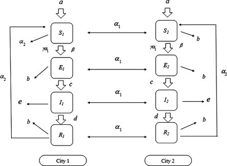
Schematic diagram of the $\mathit{SEIRS}$ model for the transmission of communicable disease during the movement of population between two cities.

3. Analysis of the model

In this section, the model (2.5) is analyzed for stability of its associated equilibrium at some different cases. In particular, the Routh–Hurwitz theorem in [1], reproduced below for convenience, will be used for the kind of the following matrix $J$:

$$J=\left(\begin{array}{cccc}\hfill a_{11}\hfill & \hfill a_{12}\hfill & \hfill a_{13}\hfill & \hfill a_{14}\hfill \\ \hfill a_{21}\hfill & \hfill a_{22}\hfill & \hfill a_{23}\hfill & \hfill a_{24}\hfill \\ \hfill 0\hfill & \hfill a_{32}\hfill & \hfill a_{33}\hfill & \hfill 0\hfill \\ \hfill 0\hfill & \hfill 0\hfill & \hfill a_{43}\hfill & \hfill {\mathit{aa}}_{44}\hfill \end{array}\right)\text{.}$$ (3.1)

Lemma 3.1

$A_1=-\mathit{tr}(J)$ , $A_2=J_1+J_2+J_3$ , $A_3=Q_1+Q_2+Q_3$ , $A_4=\mathit{det}(J)$ , where $J_1=a_{44}{a}_{33}+a_{44}{a}_{22}+a_{44}{a}_{11}+a_{33}{a}_{11}$ , $J_2=a_{33}{a}_{22}-a_{32}{a}_{23}$ , $J_3=a_{22}{a}_{11}-a_{21}{a}_{12}$ , $Q_1=-a_{44}(J_2+J_3)$ , $Q_2=-a_{33}(J_2)$ , $Q_3=-(a_{32}(a_{21}{a}_{13}+a_{43}{a}_{24})+a_{11}(a_{44}{a}_{33}-a_{32}{a}_{23}))\text{.}$ Then $J$ is stable (i.e. each eigenvalue of $J$ has negative real part) if and only if the following conditions hold:

• (i) $A_i>0$,
• (ii) $A_1{A}_2-A_3>0$,
• (iii) $A_1{A}_2{A}_3-A_3^2-A_1^2{A}_4>0$.

Remark 3.1

The characteristic polynomial of matrix $J$ in (3.1) is

$${\lambda }^4+A_1{\lambda }^3+A_2{\lambda }^2+A_3\lambda +A_4=0\text{.}$$

3.1. No individual travel

The movement of individuals is neglected, this case ${\alpha }_1=0$, then model (2.5) reduces to the $\mathit{SEIRS}$ model:

$$\begin{array}{c}\frac{\mathit{dS}}{\mathit{dt}}=a-\frac{\beta \mathit{SI}}{N}-\mathit{bS}+{\alpha }_{2}R\text{,}\hfill \\ \frac{\mathit{dE}}{\mathit{dt}}=\frac{\beta \mathit{SI}}{N}-\left(b+c\right)E\text{,}\hfill \\ \frac{\mathit{dI}}{\mathit{dt}}=\mathit{cE}-\left(e+d\right)I\text{,}\hfill \\ \frac{\mathit{dR}}{\mathit{dt}}=\mathit{dI}-\left(b+{\alpha }_2\right)R\text{.}\hfill \end{array}$$ (3.2)

From biological considerations, we study (3.2) in the closed set

$$D=\{(S\text{,}E\text{,}I\text{,}R)\in {\mathbb{R}}_{+}^4|S⩾0\text{,}E⩾0\text{,}I⩾0\text{,}R⩾0\text{,}S+E+I+R⩽a/b\}\text{,}$$

where $R_{+}^4$ denotes the non–negative cone of $R^4$ including its lower dimensional faces. It can be verified that $D$ is positively invariant with respect to (3.2).

The disease-free equilibrium, obtained by setting the right–hand sides of equations in (3.2) to zero, is given by

$$P_0(S^0\text{,}0\text{,}0\text{,}0)=\left(\frac{a}{b}\text{,}0\text{,}0\text{,}0\right)\text{.}$$ (3.3)

The linear stability of $P_0$ can be established using the next generation method [8], [10] by writing the right hand sides of second and third equation in (3.2) in term of two matrices $F$ and $V$, where $F$ is a matrix consisting of all term with $\beta$ and $V$ is M-matrix consisting of the remaining transition term in two equations (it should be recalled that a matrix A is an M-matrix if and only if every off-diagonal entry of A is non-positive and the diagonal entries are all non-negative). That is, for the model (3.2), the next generation matrices $F$ and $V$ are given by

$$F=\left(\begin{array}{cc}\hfill 0\hfill & \hfill \beta \hfill \\ \hfill 0\hfill & \hfill 0\hfill & \hfill \hfill \end{array}\right)\mathrm{and}V=\left(\begin{array}{cc}\hfill b+c\hfill & \hfill 0\hfill \\ \hfill -c\hfill & \hfill e+d\hfill \end{array}\right)\text{.}$$

Using the next generation method, the local stability of disease-free equilibrium, $P_0$, is based on whether or not $\rho ({\mathit{FV}}^{-1})<1$, where $\rho$ is the spectral radius. If $\rho ({\mathit{FV}}^{-1})<1$, then all eigenvalues of the linearized model have negative real parts, so that the disease-free equilibrium is locally asymptotically stable ($\mathit{LAS}$). For $\rho ({\mathit{FV}}^{-1})>1$, at least one of the eigenvalues of the linearization has positive real part, thus, the disease-free equilibrium is unstable in this case. Let ${\mathcal{R}}_0=\rho ({\mathit{FV}}^{-1})$, it is easy to show that

$${\mathcal{R}}_0=\frac{\beta c}{\left(e+d\right)\left(b+c\right)}\text{.}$$ (3.4)

Consequently, using Theorem 2 of [28], the following results is established.

Theorem 3.1

The disease-free equilibrium (DFE), $P_0$ , of the system ( 3.2 ) is locally asymptotically stable (LAS) if ${\mathcal{R}}_0<1$ and unstable if ${\mathcal{R}}_0>1$ .

The quantity $R_0$ in (3.4) is called the basic reproduction number of infection [2]. It is generally known that if ${\mathcal{R}}_0<1$, then the disease-free equilibrium is locally asymptotically stable (and the disease will be eradicate from the community if the initial sizes of the four state variables are within the vicinity of $P_0$). Therefore, in the event of an epidemic, the theoretical determination of conditions that can make ${\mathcal{R}}_0$ less than unity is of great public health interest. If ${\mathcal{R}}_0>1$, the system (3.2) has an endemic equilibrium $P_{\ast }(S^{\ast }\text{,}{E}^{\ast }\text{,}{I}^{\ast }\text{,}{R}^{\ast })$, where

$$S^{*}=\frac{a\left\{\left(b+{\alpha }_2\right)(c+d+e)+\mathit{cd}\right\}}{\mathrm{\Omega }}\text{,}{E}^{*}=\frac{a\left({\mathcal{R}}_0-1\right)\left(b+{\alpha }_2\right)\left(e+d\right)}{\mathrm{\Omega }}\text{,}$$ (3.5)

$$I^{*}=\frac{\mathit{ac}\left({\mathcal{R}}_0-1\right)\left(b+{\alpha }_2\right)}{\mathrm{\Omega }}\text{,}{R}^{\ast }=\frac{\mathit{acd}\left({\mathcal{R}}_0-1\right)\left(b+{\alpha }_2\right)}{\mathrm{\Omega }}\text{,}$$ (3.6)

with $\mathrm{\Omega }={\mathcal{R}}_{0}b(\mathit{be}+\mathit{cd}+d{\alpha }_2+e{\alpha }_2+\mathit{bd})+c(b+{\alpha }_2)(({\mathcal{R}}_0-1)e+b)$, and $N^{*}=S^{\ast }+E^{\ast }+I^{\ast }+R^{\ast }={\mathcal{R}}_0{S}^{\ast }\text{.}$

Evaluating the Jacobian of (3.2) at $P_{\ast }$ gives

$$J(P_{\ast })=\left(\begin{array}{cccc}\hfill -b-{\psi }_1\hfill & \hfill {\psi }_2\hfill & \hfill -{\psi }_3\hfill & \hfill {\psi }_2+{\alpha }_2\hfill \\ \hfill {\psi }_1\hfill & \hfill -b-c-{\psi }_2\hfill & \hfill {\psi }_3\hfill & \hfill -{\psi }_2\hfill \\ \hfill 0\hfill & \hfill c\hfill & \hfill -e-d\hfill & \hfill 0\hfill \\ \hfill 0\hfill & \hfill 0\hfill & \hfill d\hfill & \hfill -b-{\alpha }_2\hfill \end{array}\right)\text{,}$$ (3.7)

where

$$\begin{array}{cc}\hfill & {\psi }_1=\frac{\beta I^{\ast }(N^{\ast }-S^{\ast })}{{N^{\ast }}^2}=\frac{\beta c{\left({\mathcal{R}}_0-1\right)}^2\left(b+{\alpha }_2\right)}{{\mathcal{R}}_0^2\left((b+{\alpha }_2)(c+d+e)+\mathit{cd}\right)}\text{,}\hfill \\ \hfill & {\psi }_2=\frac{\beta S^{\ast }{I}^{\ast }}{{N^{\ast }}^2}=\frac{\beta c\left({\mathcal{R}}_0-1\right)\left(b+{\alpha }_2\right)}{{\mathcal{R}}_0^2\left((b+{\alpha }_2)(c+d+e)+\mathit{cd}\right)}\text{,}\hfill \\ \hfill & {\psi }_3=\frac{\beta S^{\ast }(N^{\ast }-I^{\ast })}{{N^{\ast }}^2}=\frac{(\beta c+\beta {\mathcal{R}}_0(d+e))(b+{\alpha }_2)+\beta \mathit{cd}{\mathcal{R}}_0}{{\mathcal{R}}_0^2\left((b+{\alpha }_2)(c+d+e)+\mathit{cd}\right)}\text{.}\hfill \end{array}$$ (3.8)

Note that Jacobian matrix (3.7) has the form as (3.1), using Lemma 3.1 (see Appendix A), we have the following result:

Theorem 3.2

If ${\mathcal{R}}_0>1$ , the endemic equilibrium, $P_{\ast }$ , is LAS.

3.2. Only susceptible and exposed individuals travel

When the infected and recovered individuals are inhibited from traveling to another city, that is ${\alpha }_1=\gamma =0$, the model (2.5) becomes

$$\begin{array}{c}\frac{{\mathit{dS}}_1}{\mathit{dt}}=a-{\mathit{bS}}_1-\frac{\beta S_1{I}_1}{N_1}+{\alpha }_2{R}_1-{\alpha }_1{S}_1+{\alpha }_1{S}_2\text{,}\hfill \\ \frac{{\mathit{dE}}_1}{\mathit{dt}}=\frac{\beta S_1{I}_1}{N_1}-\left(b+c+{\alpha }_1\right)E_1+{\alpha }_1{E}_2\text{,}\hfill \\ \frac{{\mathit{dI}}_1}{\mathit{dt}}={\mathit{cE}}_1-\left(e+d\right)I_1\text{,}\hfill \\ \frac{{\mathit{dR}}_1}{\mathit{dt}}={\mathit{dI}}_1-\left(b+{\alpha }_2\right)R_1\text{,}\hfill \\ \frac{{\mathit{dS}}_2}{\mathit{dt}}=a-{\mathit{bS}}_2-\frac{\beta S_2{I}_2}{N_2}+{\alpha }_2{R}_2-{\alpha }_1{S}_2+{\alpha }_1{S}_1\text{,}\hfill \\ \frac{{\mathit{dE}}_2}{\mathit{dt}}=\frac{\beta S_2{I}_2}{N_2}-\left(b+c+{\alpha }_1\right)E_2+{\alpha }_1{E}_1\text{,}\hfill \\ \frac{{\mathit{dI}}_2}{\mathit{dt}}={\mathit{cE}}_2-\left(e+d\right)I_2\text{,}\hfill \\ \frac{{\mathit{dR}}_2}{\mathit{dt}}={\mathit{dI}}_2-\left(b+{\alpha }_2\right)R_2\text{.}\hfill \end{array}$$ (3.9)

From calculations, there are possible two steady states for model (3.9); namely, disease-free equilibrium, $P_1(\frac{a}{b}\text{,}0\text{,}0\text{,}0\text{,}\frac{a}{b}\text{,}0\text{,}0\text{,}0)$ and endemic equilibrium, $P_2(S^{\ast }\text{,}{E}^{\ast }\text{,}{I}^{\ast }\text{,}{R}^{\ast }\text{,}{S}^{\ast }\text{,}{E}^{\ast }\text{,}{I}^{\ast }\text{,}{R}^{\ast })$, respectively. Here $S^{\ast }\text{,}{E}^{\ast }\text{,}{I}^{\ast }\text{,}{R}^{\ast }\text{,}{\mathcal{R}}_0$ are given by Eqs. (3.5), (3.6).

According to the concept of next generation matrix [8] and reproduction number presented in van den Driessche and Watmough [28], the matrices $F$ and $V$ are given by

$$F=\left(\begin{array}{cccc}\hfill 0\hfill & \hfill \beta \hfill & \hfill 0\hfill & \hfill 0\hfill \\ \hfill 0\hfill & \hfill 0\hfill & \hfill 0\hfill & \hfill 0\hfill \\ \hfill 0\hfill & \hfill 0\hfill & \hfill \beta \hfill & \hfill 0\hfill \\ \hfill 0\hfill & \hfill 0\hfill & \hfill 0\hfill & \hfill 0\hfill \end{array}\right)\mathrm{and}V=\left(\begin{array}{cccc}\hfill b+c+{\alpha }_1\hfill & \hfill 0\hfill & \hfill -{\alpha }_1\hfill & \hfill 0\hfill \\ \hfill -c\hfill & \hfill e+d\hfill & \hfill 0\hfill & \hfill 0\hfill \\ \hfill -{\alpha }_1\hfill & \hfill 0\hfill & \hfill b+c+{\alpha }_1\hfill & \hfill 0\hfill \\ \hfill 0\hfill & \hfill 0\hfill & \hfill -c\hfill & \hfill e+d\hfill \end{array}\right)\text{,}\mathrm{respectively}\text{.}$$

Therefore, the basic reproduction number of model (3.9) is given by

$${\mathcal{R}}_0^{\prime }=\rho ({\mathit{FV}}^{-1})=\frac{\beta c}{\left(e+d\right)\left(b+c\right).}$$ (3.10)

Note that the basic reproduction numbers of (3.2), (3.9) are identical.

The Jacobian matrix of the model (3.9) at equilibrium point, $P$, is given by

$$J(P)=\left(\begin{array}{cc}\hfill A_1\hfill & \hfill B\hfill \\ \hfill B\hfill & \hfill A_2\hfill \end{array}\right)$$ (3.11)

where, for $i=1\text{,}2\text{,}$

$$A_i=\left(\begin{array}{cccc}\hfill -b-{\alpha }_1-\frac{\beta I_i(N_i-S_i)}{N_i^2}\hfill & \hfill \frac{\beta S_i{I}_i}{N_i^2}\hfill & \hfill -\frac{\beta S_i(N_i-I_i)}{N_i^2}\hfill & \hfill \frac{\beta S_i{I}_i}{N_i^2}+{\alpha }_2\hfill \\ \hfill \frac{\beta I_i(N_i-S_i)}{N_i^2}\hfill & \hfill -b-c-{\alpha }_1-\frac{\beta S_i{I}_i}{N_i^2}\hfill & \hfill \frac{\beta S_i(N_i-I_i)}{N_i^2}\hfill & \hfill -\frac{\beta S_i{I}_i}{N_i^2}\hfill \\ \hfill 0\hfill & \hfill c\hfill & \hfill -e-d\hfill & \hfill 0\hfill \\ \hfill 0\hfill & \hfill 0\hfill & \hfill d\hfill & \hfill -b-{\alpha }_2\hfill \end{array}\right)$$

and $B=\left(\begin{array}{cccc}\hfill {\alpha }_1\hfill & \hfill 0\hfill & \hfill 0\hfill & \hfill 0\hfill \\ \hfill 0\hfill & \hfill {\alpha }_1\hfill & \hfill 0\hfill & \hfill 0\hfill \\ \hfill 0\hfill & \hfill 0\hfill & \hfill 0\hfill & \hfill 0\hfill \\ \hfill 0\hfill & \hfill 0\hfill & \hfill 0\hfill & \hfill 0\hfill \end{array}\right)\text{.}$ From calculations in Appendix B, the following result is established:

Theorem 3.3

(i) If ${\mathcal{R}}_0^{\prime }<1$ , then $P_1$ is LAS. (ii) If ${\mathcal{R}}_0^{\prime }>1$ , then $P_2$ is LAS.

Remark 3.2

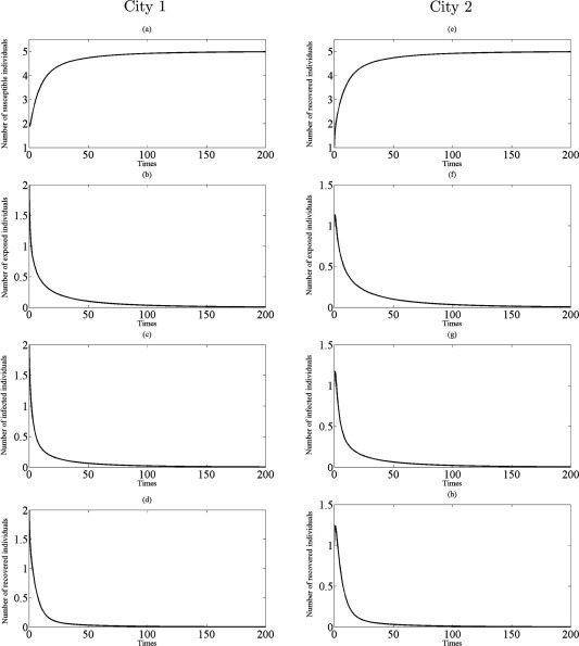
There is, from Theorem 3.3, some import implications. First, if the disease have appeared in both cities then the travel of susceptible and exposed individuals does not change the dynamics of disease spreading, and the final size of susceptible, exposed, infected and recovered individuals does not change, see Fig. 4. Second, if a disease has appeared only in city 1 with $E_1(0)>0$, $I_1(0)>0$, $E_2(0)=0$, $I_2(0)=0$ and ${\mathcal{R}}_0^{\prime }>1$ (see Figs. 4(b)–(c)), the traveling of exposed individuals will bring the disease to city 2 and the disease will break out later in city 2 (see Figs. 4(f)–(g)). On the contrary, if ${\mathcal{R}}_0^{\prime }<1$, there is not the possibility for disease spreading in both cities, as shown in Figs. 4(b)–(c)), and Figs. 3(f)–(g).

Fig. 4.

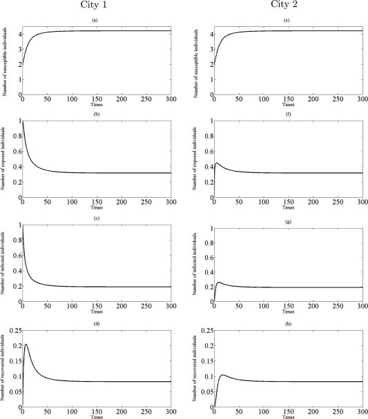
Simulations of the model (3.9) showing the number of all individuals in two cities as a function of time using the parameter values in Table 1 with $\beta =0.95$ and ${\mathcal{R}}_0^{\prime }=1.14>1$: (a)–(d) the profiles of all populations in city 1; (e)–(h) the profiles of all populations in city 2.

Fig. 3.

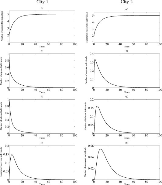
Simulations of the model (3.9) showing the number of all individuals in two cities as a function of time using the parameter values in Table 1 with $\beta =0.6$ and ${\mathcal{R}}_0^{\prime }=0.72<1$: (a)–(d) the profiles of all populations in city 1; (e)–(h) the profiles of all populations in city 2.

3.3. All individuals travel between two cities

In this section, the full model (2.5) is explored to study the effect of transport-related infection when all individuals can travel between two cities. The extended model (2.5) has a disease-free equilibrium, given by $P_1(\frac{a}{b}\text{,}0\text{,}0\text{,}0\text{,}\frac{a}{b}\text{,}0\text{,}0\text{,}0)$. Here, the next generation matrices, $F$ and $V$, are given by

$$F=\left(\begin{array}{cccc}\hfill 0\hfill & \hfill \beta \hfill & \hfill 0\hfill & \hfill \gamma {\alpha }_1\hfill \\ \hfill 0\hfill & \hfill 0\hfill & \hfill 0\hfill & \hfill 0\hfill \\ \hfill 0\hfill & \hfill \gamma {\alpha }_1\hfill & \hfill 0\hfill & \hfill \beta \hfill \\ \hfill 0\hfill & \hfill 0\hfill & \hfill 0\hfill & \hfill 0\hfill \end{array}\right)\mathrm{and}V=\left(\begin{array}{cccc}\hfill b+c+{\alpha }_1\hfill & \hfill 0\hfill & \hfill -{\alpha }_1\hfill & \hfill 0\hfill \\ \hfill -c\hfill & \hfill e+d+{\alpha }_1\hfill & \hfill 0\hfill & \hfill -{\alpha }_1\hfill \\ \hfill -{\alpha }_1\hfill & \hfill 0\hfill & \hfill b+c+{\alpha }_1\hfill & \hfill 0\hfill \\ \hfill 0\hfill & \hfill -{\alpha }_1\hfill & \hfill -c\hfill & \hfill e+d+{\alpha }_1\hfill \end{array}\right)\text{.}$$

It follows that, using the next generation approach, the basic reproduction number of the model (2.5), denoted by ${\mathcal{R}}_{0\gamma }$, is

$${\mathcal{R}}_{0\gamma }={\mathcal{R}}_0+\frac{\gamma {\alpha }_{1}c}{(b+c)(d+e)}\text{.}$$ (3.12)

Consequently, using Theorem 2 of [28], the following result is established.

Lemma 3.2

The disease-free equilibrium, $P_1$ , of the model (2.5) is LAS if ${\mathcal{R}}_{0\gamma }<1$ , and unstable if ${\mathcal{R}}_{0\gamma }>1$.

The model (2.5) has a unique coexistence endemic equilibrium denoted by $P_{\gamma }^{\ast }(S_{\gamma }^{\ast }\text{,}{E}_{\gamma }^{\ast }\text{,}{I}_{\gamma }^{\ast }\text{,}{R}_{\gamma }^{\ast }\text{,}{S}_{\gamma }^{\ast }\text{,}{E}_{\gamma }^{\ast }\text{,}{I}_{\gamma }^{\ast }\text{,}{R}_{\gamma }^{\ast })$,

$$S_{\gamma }^{*}=\frac{a\left\{\left(b+{\alpha }_2\right)(c+d+e)+\mathit{cd}\right\}}{{\mathrm{\Omega }}_{\gamma }}\text{,}{E}_{\gamma }^{*}=\frac{a\left({\mathcal{R}}_{0\gamma }-1\right)\left(b+{\alpha }_2\right)\left(e+d\right)}{{\mathrm{\Omega }}_{\gamma }}\text{,}$$ (3.13)

$$I_{\gamma }^{*}=\frac{\mathit{ac}\left({\mathcal{R}}_{0\gamma }-1\right)\left(b+{\alpha }_2\right)}{{\mathrm{\Omega }}_{\gamma }}\text{,}{R}_{\gamma }^{*}=\frac{\mathit{acd}\left({\mathcal{R}}_{0\gamma }-1\right)\left(b+{\alpha }_2\right)}{{\mathrm{\Omega }}_{\gamma }}\text{,}$$ (3.14)

with ${\mathrm{\Omega }}_{\gamma }={\mathcal{R}}_{0\gamma }b(\mathit{be}+\mathit{cd}+d{\alpha }_2+e{\alpha }_2+\mathit{bd})+c(b+{\alpha }_2)(({\mathcal{R}}_{0\gamma }-1)e+b)\text{.}$

The local stability of the coexistence endemic equilibrium is now explored. The Jacobian matrix of system (2.5) at the equilibrium point, $P$, is given by

$$J(P)=\left(\begin{array}{cc}\hfill A_1\hfill & \hfill B_2\hfill \\ \hfill B_1\hfill & \hfill A_2\hfill \end{array}\right)\text{,}$$ (3.15)

where, for $i=1\text{,}2$, $N_i=S_i+E_i+I_i+R_i$,

$$A_i=\left(\begin{array}{cccc}\hfill -b-{\alpha }_1-\frac{\beta I_i(N_i-S_i)}{N_i^2}\hfill & \hfill \frac{\beta S_i{I}_i}{N_i^2}\hfill & \hfill -\frac{\beta S_i(N_i-I_i)}{N_i^2}\hfill & \hfill \frac{\beta S_i{I}_i}{N_i^2}+{\alpha }_2\hfill \\ \hfill \frac{\beta I_i(N_i-S_i)}{N_i^2}\hfill & \hfill -b-c-{\alpha }_1-\frac{\beta S_i{I}_i}{N_i^2}\hfill & \hfill \frac{\beta S_i(N_i-I_i)}{N_i^2}\hfill & \hfill -\frac{\beta S_i{I}_i}{N_i^2}\hfill \\ \hfill 0\hfill & \hfill c\hfill & \hfill -e-d-{\alpha }_1\hfill & \hfill 0\hfill \\ \hfill 0\hfill & \hfill 0\hfill & \hfill d\hfill & \hfill -b-{\alpha }_1-{\alpha }_2\hfill \end{array}\right)$$

and

$$B_i=\left(\begin{array}{cccc}\hfill {\alpha }_1-\frac{\gamma {\alpha }_1{I}_i(N_i-S_i)}{N_i^2}\hfill & \hfill \frac{\gamma {\alpha }_1{S}_i{I}_i}{N_i^2}\hfill & \hfill -\frac{\gamma {\alpha }_1{S}_i(N_i-I_i)}{N_i^2}\hfill & \hfill \frac{\gamma {\alpha }_1{S}_i{I}_i}{N_i^2}\hfill \\ \hfill \frac{\gamma {\alpha }_1{I}_i(N_i-S_i)}{N_i^2}\hfill & \hfill {\alpha }_1-\frac{\gamma {\alpha }_1{S}_i{I}_i}{N_i^2}\hfill & \hfill \frac{\gamma {\alpha }_1{S}_i(N_i-I_i)}{N_i^2}\hfill & \hfill -\frac{\gamma {\alpha }_1{S}_i{I}_i}{N_i^2}\hfill \\ \hfill 0\hfill & \hfill 0\hfill & \hfill {\alpha }_1\hfill & \hfill 0\hfill \\ \hfill 0\hfill & \hfill 0\hfill & \hfill 0\hfill & \hfill {\alpha }_1\hfill \end{array}\right)\text{.}$$

From calculations in Appendix C, we have the following results:

Theorem 3.4

The endemic equilibrium, $P_{\gamma }^{\ast }$ , of (2.5) is LAS if ${\mathcal{R}}_{0\gamma }>1\text{.}$

From Theorem 3.4, the disease eradication is possible for a sufficient small parameter $\gamma$ when the both cities are disease-free without traveling (that is, ${\mathcal{R}}_{0\gamma }<1$ for small $\gamma$ when ${\mathcal{R}}_0<1$). Comparing ${\mathcal{R}}_{0\gamma }$ with ${\mathcal{R}}_0$, on the other hand, we find that even a small transmission rate $\gamma$ is unfavorable or harmful to disease eradication since ${\mathcal{R}}_{0\gamma }>{\mathcal{R}}_0$ for $\gamma >0$. In fact, if $\gamma =0$ and ${\mathcal{R}}_0<1$ hold, then infectious disease should disappear in both cities from (3.12) (see Fig. 5, Fig. 6). Further, if infected individuals can travel and there is transport-related infection such that ${\mathcal{R}}_{0\gamma }>1$ then the endemic steady state $P_{\gamma }^{\ast }(S_{\gamma }^{\ast }\text{,}{E}_{\gamma }^{\ast }\text{,}{I}_{\gamma }^{\ast }\text{,}{R}_{\gamma }^{\ast }\text{,}{S}_{\gamma }^{\ast }\text{,}{E}_{\gamma }^{\ast }\text{,}{I}_{\gamma }^{\ast }\text{,}{R}_{\gamma }^{\ast })$ appears in two cities to become stable. This situation is illustrated in Fig. 7, Fig. 8.

Fig. 5.

Simulations of the model (2.5) showing the number of all individuals in two cities as a function of time using the parameter values in Table 1 with $\beta =0.6$, $\gamma =0.09$, ${\mathcal{R}}_0=0.72<1$ and ${\mathcal{R}}_{0\gamma }=0.82<1$: (a)–(d) the profiles of all populations in city 1; (e)–(h) the profiles of all populations in city 2.

Fig. 6.

Simulations of the model (2.5) showing the number of all individuals in two cities as a function of time using the parameter values in Table 1 with $\beta =0.6$, $\gamma =0.2$, ${\mathcal{R}}_0=0.72<1$ and ${\mathcal{R}}_{0\gamma }=0.936<1$: (a)–(d) the profiles of all populations in city 1; (e)–(h) the profiles of all populations in city 2.

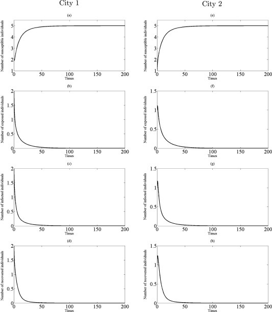
Fig. 7.

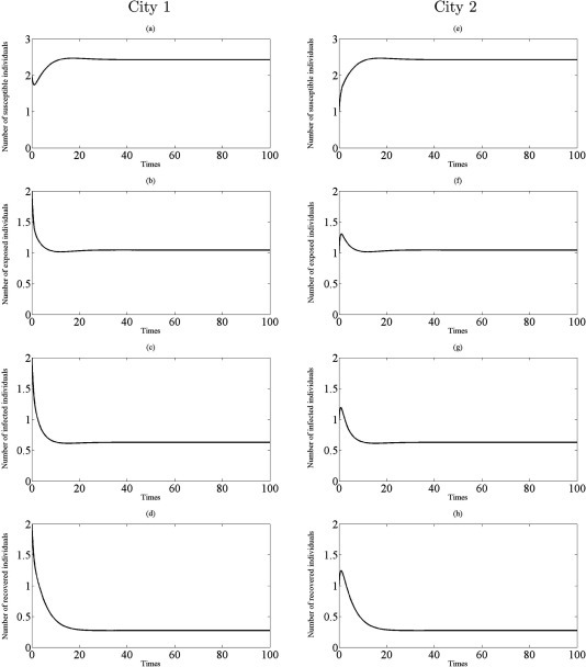
Simulations of the model (2.5) showing the number of all individuals in two cities as a function of time using the parameter values in Table 1 with $\beta =0.6$, $\gamma =1$, ${\mathcal{R}}_0=0.72<1$ and ${\mathcal{R}}_{0\gamma }=1.8>1$: (a)–(d) the profiles of all populations in city 1; (e)–(h) the profiles of all populations in city 2.

Fig. 8.

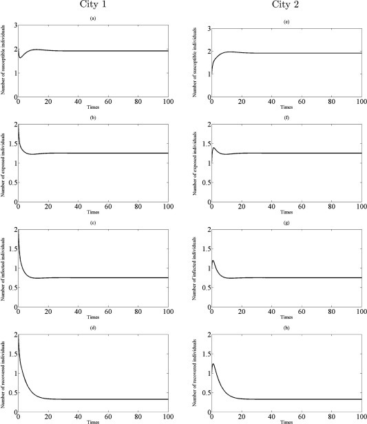
Simulations of the model (2.5) showing the number of all individuals in two cities as a function of time using the parameter values in Table 1 with $\beta =0.95$, $\gamma =1$, ${\mathcal{R}}_0=1.14>1$ and ${\mathcal{R}}_{0\gamma }=2.22>1$: (a)–(d) the profiles of all populations in city 1; (e)–(h) the profiles of all populations in city 2.

As above results, it can be concluded that if the disease is endemic in both isolated cities, then transport-related infection will surely lead to the disease becoming endemic. When the two isolated cities are disease-free, transport-related infection may also have the possibility to lead to the disease becoming endemic. In addition, to see clearly the effect of transport-related infection, the relations among two reproduction number, ${\mathcal{R}}_0$ in (3.4) and ${\mathcal{R}}_{0\gamma }$ in (3.12), are compared. It is found that ${\mathcal{R}}_{0\gamma }>{\mathcal{R}}_0$ for $\gamma >0$, and ${\mathcal{R}}_{0\gamma }={\mathcal{R}}_0$ for $\gamma =0$. Since $\frac{\partial {\mathcal{R}}_{0\gamma }}{\partial \gamma }=\frac{{\alpha }_1}{(b+c)(e+d)}>0$ for all $\gamma >0$, it implies that ${\mathcal{R}}_{0\gamma }$ increases with the increase of $\gamma$. Consider the coexistence steady state $P_{\gamma }^{\ast }(S_{\gamma }^{\ast }\text{,}{E}_{\gamma }^{\ast }\text{,}{I}_{\gamma }^{\ast }\text{,}{R}_{\gamma }^{\ast }\text{,}{S}_{\gamma }^{\ast }\text{,}{E}_{\gamma }^{\ast }\text{,}{I}_{\gamma }^{\ast }\text{,}{R}_{\gamma }^{\ast })$ of the model (2.5) given by Eqs. (3.13), (3.14), it is clear that $S_{\gamma }^{\ast }\to S^{\ast }$, $E_{\gamma }^{\ast }\to E^{\ast }$, $I_{\gamma }^{\ast }\to I^{\ast }$, $R_{\gamma }^{\ast }\to R^{\ast }$ as $\gamma \to 0$. Comparing coexistence steady state values of susceptible, exposed, infected and recovered individuals in the case of $\gamma =0$ with those of $\gamma >0$, respectively, give $S_{\gamma }^{\ast }<S^{\ast }$, $E_{\gamma }^{\ast }>E^{\ast }$, $I_{\gamma }^{\ast }>I^{\ast }$ and $R_{\gamma }^{\ast }>R^{\ast }$ for $\gamma >0$ because of

$$\begin{array}{cc}\hfill & \frac{\partial S_{\gamma }^{\ast }}{\partial \gamma }=-\frac{a[(b+{\alpha }_2)(c+d+e)+\mathit{cd}]\partial {\mathcal{R}}_{0\gamma }/\partial \gamma }{{\mathrm{\Omega }}_{\gamma }^2}<0\text{,}\hfill \\ \hfill & \frac{\partial E_{\gamma }^{\ast }}{\partial \gamma }=\frac{a\mathrm{\Lambda }(b+{\alpha }_2)(e+d)\partial {\mathcal{R}}_{0\gamma }/\partial \gamma }{{\mathrm{\Omega }}_{\gamma }^2}>0\text{,}\hfill \\ \hfill & \frac{\partial I_{\gamma }^{\ast }}{\partial \gamma }=\frac{\mathit{ac}\mathrm{\Lambda }(b+{\alpha }_2)\partial {\mathcal{R}}_{0\gamma }/\partial \gamma }{{\mathrm{\Omega }}_{\gamma }^2}>0\text{,}\hfill \\ \hfill & \frac{\partial R_{\gamma }^{\ast }}{\partial \gamma }=\frac{\mathit{ac}\mathrm{\Lambda }(b+{\alpha }_2)\partial {\mathcal{R}}_{0\gamma }/\partial \gamma }{{\mathrm{\Omega }}_{\gamma }^2}>0\text{,}\hfill \end{array}$$

with $\mathrm{\Lambda }=b(\mathit{bc}+c{\alpha }_2+\mathit{be}+\mathit{cd}+d{\alpha }_2+e{\alpha }_2+\mathit{bd})$. It is also found that $S_{\gamma }^{\ast }=S^{\ast }$, $E_{\gamma }^{\ast }=E^{\ast }$, $I_{\gamma }^{\ast }=I^{\ast }$ and $R_{\gamma }^{\ast }=R^{\ast }$ when $\gamma =0$. This implies that, at steady–state, the total number of susceptible individuals in the both cities decreases with the increase of $\gamma$, while the total number of exposed, infected and recovered individuals increase with the increase of $\gamma$.

Next, the effect of transport-related infection to the final size of population is discussed. Note that

$$N_{\gamma }^{\ast }=S_{\gamma }^{\ast }+E_{\gamma }^{\ast }+I_{\gamma }^{\ast }+R_{\gamma }^{\ast }=\frac{a[(b+{\alpha }_2)(c+d+e)+\mathit{cd}]}{\mathrm{\Delta }+\aleph }\text{,}$$ (3.16)

where $\mathrm{\Delta }=b(\mathit{be}+\mathit{cd}+d{\alpha }_2+e{\alpha }_2+\mathit{bd}+\mathit{ce})+\mathit{ce}{\alpha }_2$ and $\aleph =\frac{c(b+{\alpha }_2)(b-e)(e+d)(b+c)}{\beta +\gamma {\alpha }_1}$.

The partial derivative of $N_{\gamma }^{\ast }$ with respect to $\gamma$ is given by

$$\frac{\partial N_{\gamma }^{\ast }}{\partial \gamma }=-\frac{a[(b+{\alpha }_2)(c+d+e)+\mathit{cd}]}{{(\mathrm{\Delta }+\aleph )}^2}\frac{\partial \aleph }{\partial \gamma }$$

with

$$\frac{\partial \aleph }{\partial \gamma }=\frac{c{\alpha }_1(b+{\alpha }_2)(e-b)(e+d)(b+c)}{{(\beta +\gamma {\alpha }_1)}^2}\text{.}$$

Since $e>b$ then $\frac{\partial \aleph }{\partial \gamma }>0$. It follows that $\frac{\partial N_{\gamma }^{\ast }}{\partial \gamma }<0\text{.}$ Therefore, $N_{\gamma }^{\ast }<N^{\ast }$ for $\gamma >0$ and $N_{\gamma }^{\ast }=N^{\ast }$ for $\gamma =0$. This implies that the final size of populations decreases with the increase of $\gamma$.

By the way, it is found that

$$\begin{array}{cc}\hfill & \frac{\partial }{\partial \gamma }\left(\frac{E_{\gamma }^{\ast }+I_{\gamma }^{\ast }+R_{\gamma }^{\ast }}{N_{\gamma }^{\ast }}\right)=\frac{1}{{N_{\gamma }^{\ast }}^2}\left[\frac{\partial (E_{\gamma }^{\ast }+I_{\gamma }^{\ast }+R_{\gamma }^{\ast })}{\partial \gamma }{S}_{\gamma }^{\ast }-\frac{\partial S_{\gamma }^{\ast }}{\partial \gamma }(E_{\gamma }^{\ast }+I_{\gamma }^{\ast }+R_{\gamma }^{\ast })\right]>0\text{,}\hfill \\ \hfill & \frac{\partial }{\partial \gamma }\left(\frac{S_{\gamma }^{\ast }}{N_{\gamma }^{\ast }}\right)=\frac{1}{{N_{\gamma }^{\ast }}^2}\left[\frac{\partial S_{\gamma }^{\ast }}{\partial \gamma }(E_{\gamma }^{\ast }+I_{\gamma }^{\ast }+R_{\gamma }^{\ast })-S_{\gamma }^{\ast }\frac{\partial (E_{\gamma }^{\ast }+I_{\gamma }^{\ast }+R_{\gamma }^{\ast })}{\partial \gamma }\right]<0\text{,}\hfill \end{array}$$

since $\frac{\partial S_{\gamma }^{\ast }}{\partial \gamma }<0$. These imply that the proportion of the total number of exposed, infected and recovered individuals (i.e. the total number of individuals affected by the disease) increases with the increase of $\gamma$. On the contrary, the proportion of the susceptible individuals decreases with the increase of $\gamma$. Therefore, as above described, it can be suggested that transport-related infection will cause an endemic disease more seriously on spreading disease. Moreover, from these epidemiological implications, it is very essential to strengthen restrictions of passengers once when an infectious disease appears.

4. Numerical experiments

The models (2.5), (3.2), (3.9) are solved by using fourth–order Runge kutta method with the parameter values/ranges in Table 1 . The results are shown in two experiments. Experiment 1 presents the various theoretical results under the conditions of the basic reproduction numbers, ${\mathcal{R}}_0$ and ${\mathcal{R}}_{0\gamma }$, in order to illustrate the effect of transport-related infection on its outbreak. Experiment 2 shows the $\mathit{SEIRS}$ model (3.2) is applied to study the outbreak of SARS in a city and the $\mathit{SEIRS}$ model with transport-related infection (2.5) is applied to study the SARS outbreak during the movement between two cities.

Table 1.

Description and parameter values for the models (2.5), (3.2), (3.9).

Parameters	Descriptions	Values	References
$a$	Recruitment rate	1	[29]
	(by birth and by immigration)
$b$	Natural death rate	0.2	[29]
$c$	Rate that exposed individuals	0.3	[29]
	become infected individuals
$d$	Transfer rate from infected	0.1	[22]
	individuals to recovered individuals
$e$	Mortality rate for infected individuals	0.4	[29]
${\alpha }_2$	Rate that recovered individuals	0.03	[22]
	become susceptible individuals
${\alpha }_1$	Rate that individuals of city $i$ leave	0.9	[29]
	to city $j(j\ne i)$
$\beta$	Transmission rate	$0⩽\beta \le 1$	Assumed
$\gamma$	Transport-related transmission rate	$0⩽\gamma \le 1$	Assumed

4.1. Experiment 1: numerical simulations of the models

Firstly, the dynamics of model (3.2) which neglects the movement of individuals are investigated by setting the transmission rate within a city, $\beta =0.6$, 0.95 due to give ${\mathcal{R}}_0=0.72<1$ and ${\mathcal{R}}_0=1.14>1$, respectively. The typical behaviors of all individuals at steady-states as a function of ${\mathcal{R}}_0$ are shown in Fig. 2 . Figs. 2(a)–(d) verifies that the numerical solutions of the model (3.2) converge to disease-free equilibrium, $P_0(S^0\text{,}0\text{,}0\text{,}0)$, whenever ${\mathcal{R}}_0<1$, and to endemic equilibrium in (3.5), (3.6), $P_{\ast }(4.219\text{,}0.317\text{,}0.19\text{,}0.083)$, if ${\mathcal{R}}_0>1$, (see Figs. 2(e)–(h)), respectively. These results are in line with Theorem 3.1, Theorem 3.2, respectively.

Fig. 2.

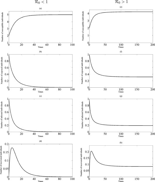
Time series plot of the model (3.2) with parameter values in Table 1 and initial conditions $S(0)=2$, $E(0)=1$, $I(0)=1$, $R(0)=0$: (a)–(d) profiles of all populations for $\beta$ = 0.6, ${\mathcal{R}}_0=0.72<1$; (e)–(h) profiles of all populations for $\beta$ = 0.95, ${\mathcal{R}}_0=1.14>1$.

Next, assume that only susceptible and exposed individuals travel to another city at the same rate ${\alpha }_1$ while the infected and recovered individuals are inhibited from traveling to another city. Thus, model (3.2) is extend to model (3.9). The model (3.9) is simulated with parameter values in Table<br/>1. For numerical simulation purposes, the transmission rate within a city, $\beta$, is set to be 0.6 and 0.95, respectively. The initial conditions are used: $S_1(0)=2$, $E_1(0)=1$, $I_1(0)=1$, $R_1(0)=0$, $S_2(0)=2$, $E_2(0)=0$, $I_2(0)=0$ and $R_2(0)=0$. The profiles of susceptible, exposed, infected and recovered individuals at steady–state are depicted in Fig. 3, Fig. 4 . Let $\beta =0.6$, then ${\mathcal{R}}_0^{\prime }=0.72$. It is seen that the obtained results convergence to the disease-free equilibrium $P_1=(S^0\text{,}0\text{,}0\text{,}0\text{,}{S}^0\text{,}0\text{,}0\text{,}0)=(5\text{,}0\text{,}0\text{,}0\text{,}5\text{,}0\text{,}0\text{,}0)$ if ${\mathcal{R}}_0^{\prime }<1$, as shown in Fig. 3. According to Theorem 3.3, the disease-free equilibrium $P_1$ is locally asymptotically stable whenever ${\mathcal{R}}_0^{\prime }<1$. It interprets that the infected individuals in city 1 decrease while the infected individuals in city 2 appear to be pandemic initially, and are eventually extinct. Therefore, the disease die out separately in two cities if ${\mathcal{R}}_0^{\prime }<1$. When $\beta =0.95$, then ${\mathcal{R}}_0=1.14$. All solutions of the model (3.9) admit an endemic equilibrium $P_2=(S^{\ast }\text{,}{E}^{\ast }\text{,}{I}^{\ast }\text{,}{R}^{\ast }\text{,}{S}^{\ast }\text{,}{E}^{\ast }\text{,}{I}^{\ast }\text{,}{R}^{\ast })=(4.219\text{,}0.317\text{,}0.19\text{,}0.083\text{,}4.219\text{,}0.317\text{,}0.19\text{,}0.083)$, see Fig. 4. This confirms that the endemic equilibrium, $P_2$, is locally asymptotically stable whenever ${\mathcal{R}}_0^{\prime }>1$ (as guaranteed by Theorem 3.3).

Finally, two basic reproductions numbers, ${\mathcal{R}}_0$ and ${\mathcal{R}}_{0\gamma }$, are compared,

$${\mathcal{R}}_0=\frac{\beta c}{\left(b+c\right)\left(e+d\right)}\mathrm{and}{\mathcal{R}}_{0\gamma }={\mathcal{R}}_0+\frac{\gamma {\alpha }_{1}c}{(b+c)(e+d)}\text{.}$$ (4.17)

It is clear that, from (4.17), ${\mathcal{R}}_{0\gamma }>{\mathcal{R}}_0$, and ${\mathcal{R}}_{0\gamma }$ depends on ${\mathcal{R}}_0$ and transport-related infection rate, $\gamma$. When $\beta =0.6$ and the other parameters $b\text{,}c\text{,}d\text{,}e\text{,}{\alpha }_1$ given in Table 1, it is found that ${\mathcal{R}}_0<1$ and ${\mathcal{R}}_{0\gamma }<1$ whenever $0<\gamma <7/27$, and ${\mathcal{R}}_0>1$ and ${\mathcal{R}}_{0\gamma }>1$ whenever $7/27<\gamma \le 1$. Whereas $\beta =0.95$ then ${\mathcal{R}}_0>1$ and ${\mathcal{R}}_{0\gamma }>1$ for all $\gamma >0$. Thus, this experiment investigates the dynamics of disease transmission into two cases by solving model (2.5) with various values of $\beta$ and $\gamma$: $\beta =0.6\text{,}0.95$ and $\gamma =0.09\text{,}0.2\text{,}1$, whilst retaining the same values of the other parameters. In all computations, the initial conditions are taken to be $S_1(0)=2$, $E_1(0)=2$, $I_1(0)=2$, $R_1(0)=2$, $S_2(0)=1$, $E_2(0)=1$, $I_2(0)=1$, $R_2(0)=1$.

• Case 1.

  When ${\mathcal{R}}_0<1$ and ${\mathcal{R}}_{0\gamma }<1$, the parameters $\beta$ and $\gamma$ are chosen to be $\beta =0.6$ and $\gamma =0.09\text{,}0.2$, respectively. The profiles of susceptible, exposed, infected and recovered individuals, as depicted in Fig. 5, Fig. 6 , reveal that the numerical solutions of model (2.5) converge to disease-free equilibrium, $P_1$, whenever ${\mathcal{R}}_{0\gamma }<1$ (as guaranteed by Lemma 3.2). This study suggests that the transport-related infection may not lead to the disease becoming endemic when ${\mathcal{R}}_0<1$ and ${\mathcal{R}}_{0\gamma }<1$ for small $\gamma$.

• Case 2.

  Taking the values of $\gamma =1$, $\beta =0.6$ and $\gamma =1$, $\beta =0.95$ give ${\mathcal{R}}_0=0.72$, ${\mathcal{R}}_{0\gamma }=1.8$ and ${\mathcal{R}}_0=1.14$, ${\mathcal{R}}_{0\gamma }=2.22$, respectively. These lead to study the dynamics of model (2.5) in the cases ${\mathcal{R}}_0<1<{\mathcal{R}}_{0\gamma }$, and $1<{\mathcal{R}}_0<{\mathcal{R}}_{0\gamma }$. All experiments are guaranteed by Theorem 3.4 in the way that the number of all individuals asymptotically approach to coexistence endemic equilibrium for ${\mathcal{R}}_{0\gamma }>1$, see Fig. 7, Fig. 8 . Therefore, the results suggest that if there is transport – related infection such that ${\mathcal{R}}_{0\gamma }>1$, then the disease is endemic in both two cities.

4.2. Experiment 2: effect of transport-related infection to SARS outbreak in Hongkong 2003

The $\mathit{SEIRS}$ model (3.2) is first applied to study the SARS outbreak in Hongkong 2003 by adding the cumulative number of SARS cases [5] which is given by

$$C^{\prime }=\mathit{kI}\text{,}$$ (4.18)

where $C$ denotes cumulative number of SARS cases and $k$ is the rate of progression from infective to diagnosed. Simulations are obtained by choosing the most proper parameters (base-case estimates) to SARS on 17 March 2003 to 26 April 2003 [35]:

$$\begin{array}{c}a=3{\mathrm{day}}^{-1}\text{,}b=0.000034{\mathrm{day}}^{-1}\text{,}c=\frac{1}{6.4}{\mathrm{day}}^{-1}\text{,}d=\frac{1}{4}{\mathrm{day}}^{-1}\text{,}\hfill \\ e=0.007934{\mathrm{day}}^{-1}\text{,}{\alpha }_2=0.001{\mathrm{day}}^{-1}\mathrm{and}k=\frac{1}{3}{\mathrm{day}}^{-1}\text{.}\hfill \end{array}$$ (4.19)

The values of $b$, $c$ and $d$ correspond to life expectancy of 80 years [13], an average incubation period of 6.4 days and infectious period of approximately 4 days [9], respectively. The rate of SARS induced mortality is 0.0079 ${\mathrm{day}}^{-1}$ [13]. The rate $k$ is progression from infective to diagnosed and is set to be 1/3 ${\mathrm{day}}^{-1}$ [5]. The natural death rate is 0.000034 ${\mathrm{day}}^{-1}$ [13], then the rate $e$ is 0.007934 ${\mathrm{day}}^{-1}$ (summation of natural death rate and SARS induced mortality rate). The basic reproduction number (${\mathcal{R}}_0$) values for SARS is in the range 2.2 to 3.7 [19], then ${\mathcal{R}}_0$ is selected as 2.7 [19]. Substituting ${\mathcal{R}}_0=2.7$ in (3.4) give the transmission rate

$$\beta =0.679{\mathrm{day}}^{-1}\text{.}$$ (4.20)

For numerical simulations, the initial conditions are assumed to be $S(0)=1\text{,}100$, $E(0)=95$, $I(0)$, $R(0)=0$ and $C(0)=95$. For $I(0)=95$ corresponds to number of infectious cases on 17 March 2003. The numerical results of model (3.2), (4.18) are shown in Fig. 9, Fig. 10 . Fig. 9 shows that the number of susceptible individuals decrease whereas the number of exposed, infected and recovered individuals increase. This means that when the disease spread occurs, the number of susceptible individuals decrease since the susceptible individuals contact with infected individuals. Thus, susceptible individuals can require exposed individuals. After 2–10 days [9], the exposed individuals is progression to symptoms development, therefore, exposed individual is called infected individuals. After that infected individuals is hospitalized about 3–5 days [9] and then infected individuals is becomes recovered individuals. It can be concluded that SARS is highly infectious base on the gradient of the susceptible curve. Fig. 10 shows the predicted total cases obtained by (4.18). The resulting curve for $C$ fits very well with the observed total cases from 17 March 2003 to 26 April 2003 (totally 54 days). This implies that $\mathit{SEIRS}$ model (3.2) can be used to predict the SARS transmission in Hongkong 2003.

Fig. 9.

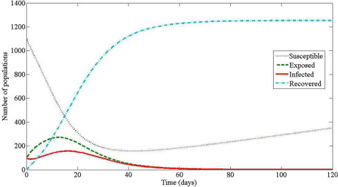
The number of all populations in a city produced by the model (3.2) with the parameter values: $a=3{\mathrm{day}}^{-1}$, $b=0.000034{\mathrm{day}}^{-1}$, $c=\frac{1}{6.4}{\mathrm{day}}^{-1}$, $d=\frac{1}{4}{\mathrm{day}}^{-1}$, $e=0.007934{\mathrm{day}}^{-1}$, ${\alpha }_2=0.001{\mathrm{day}}^{-1}$, $k=\frac{1}{3}{\mathrm{day}}^{-1}$ and $\beta =0.679{\mathrm{day}}^{-1}$.

Fig. 10.

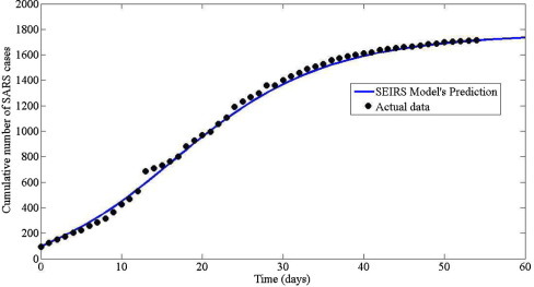
Comparison the cumulative numbers of SARS between actual data by WHO [35] (dotted lines) and predicted by $\mathit{SEIRS}$ model(3.2) (solid lines).

Next, an $\mathit{SEIRS}$ model with transport-related infection (2.5) is applied to study the dynamic of SARS during the movement among two cities. It is assumed that the all individuals can travel from one city to another city at the rate ${\alpha }_1$. It is also assumed that both cities are identical, i.e. the demographic are the same for each city. When the disease spread occurs, the disease is transmitted with transition rate $\gamma {\alpha }_1$. Thus, the effect of transport-related infection, $\gamma$, is monitored to forecast the total number of infected individuals and duration of its outbreak. In this case the model (2.5) is simulated by using parameter values ${\alpha }_1=0.9$ and various values of $\gamma$: $\gamma =0$, $\gamma =0.2$ and $\gamma =1$, whilst retaining the same values of other parameters in the previous experiment. The initial conditions are used $S_1(0)=1\text{,}100$, $E_1(0)=95$, $I_1(0)=95$, $R_1(0)=0$, $C_1(0)=95$, $S_2(0)=1\text{,}100$, $E_2(0)=5$, $I_2(0)=5$, $R_2(0)=0$, $C_2(0)=0$. The cumulative number of cases and trajectory of infected individuals, in two cities, are shown in Fig. 11, Fig. 12 , respectively. The results show that the total number of SARS in both cities increases with increase of $\gamma$ (see Fig. 11). It is also seen that the maximum number of infected individuals are 130, 150, 240 and the outbreak reached its peak about 22 days, 20 days, 10 days as $\gamma$ increase, $\gamma =0$, $\gamma =0.2$, $\gamma =1$, respectively (see Fig. 12). This confirms that the size and duration of an outbreak can be influenced by transport-related infection. Thus, to reduction and to prevention the spread of SARS, it should have the control measure of the traveling of individual from one city to another city.

Fig. 11.

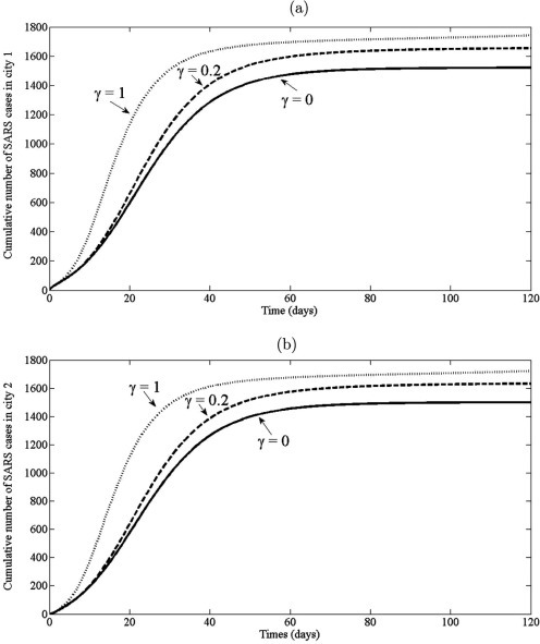
The cumulative number of SARS cases obtained by the model (2.5) with various of $\gamma$: $\gamma =0$, $\gamma =0.2$, $\gamma =1$: (a) the cumulative number of SARS cases in city 1; (b) the cumulative number of SARS cases in city 2.

Fig. 12.

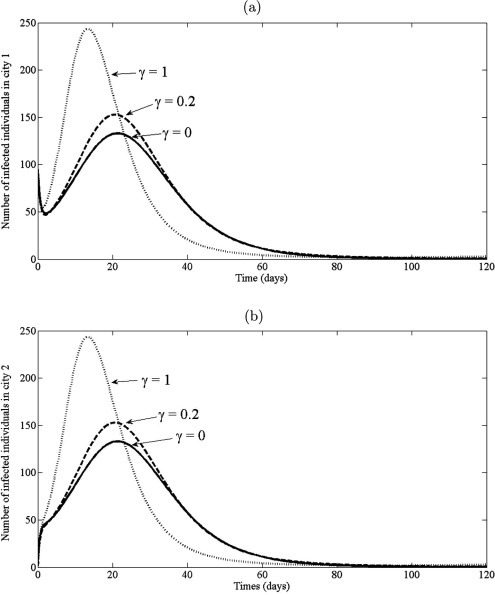
The trajectory of infected individuals of the model (2.5) with various of $\gamma$ and other parameter values: $a=3{\mathrm{day}}^{-1}$, $b=0.000034{\mathrm{day}}^{-1}$, $c=\frac{1}{6.4}{\mathrm{day}}^{-1}$, $d=\frac{1}{4}{\mathrm{day}}^{-1}$, $e=0.007934{\mathrm{day}}^{-1}$, ${\alpha }_2=0.001{\mathrm{day}}^{-1}$, $k=\frac{1}{3}{\mathrm{day}}^{-1}$, $\beta =0.679{\mathrm{day}}^{-1}$, and ${\alpha }_1=0.9{\mathrm{day}}^{-1}$.

5. Conclusions

This paper presents an $\mathit{SEIRS}$ with transport-related infection for studying the spreading disease during the movement between two cities. The model was rigorously analyzed into three cases in order to gain insights into their qualitative dynamics. The following results are obtained:

• (i)Each of the three models considered in this study has a locally asymptotically stable if a certain threshold quantity, known as the basic reproduction number, is less than unity; indicating that the number of infectious individual in the community will be brought to zero if public health measures that make (and keep) the threshold to a value less than unity are carried out;
• (ii)The basic reproduction number of the models (3.2), (3.9) are identical, then the traveling of susceptible and exposed (means exposed but not yet infectious) individuals does not change the dynamics of the corresponding epidemic model when the disease had appeared in both regions. But if the basic reproduction number is greater than unity, the traveling of the exposed individuals can bring the disease from one region to other regions according to Theorem 3.3;
• (iii)If there is no restriction on the traveling of the exposed and infectious individuals, according to Theorem 3.7 and the discussion behind this theorem, then transport-related infection intensifies the disease spread in the sense of that both the absolute and relative size of patients increase when $R_{0\gamma }>1$;
• (iv)The result of the $\mathit{SEIRS}$ model without transport related infections (3.2) is good agreement with the real data of SARS outbreak in Hongkong 2003. When there is the movement of exposed and infectious individuals between two cities, the $\mathit{SEIRS}$ model with transport related infection (2.5) is used to investigate the outbreak of SARS when the individuals in one city travel to another city. The results show that the transport-related infection is effected to the number of infected individuals and the duration of outbreak in such the way that the disease becomes more endemic due to the movement between two cities. This study can be helpful in providing the information to public health authorities and policy maker to reduce spreading disease when its occurs. However, the results of the model (2.5) has not yet forecasted the real size of the SARS epidemics in two city and one can see that in the model (2.5), it is assumed that the two regions share an identical parameter set. It may be necessary to consider two different population sizes and different dispersal rates in order to discuss precisely the impact of the transport-related infection on the disease dynamics. Moreover, to make the model more realistic, gravity models introduced by Murray and Cliff [15] is applied. We leave these to future work.

Appendix A. Proof of Theorem 3.2

Proof

From Jacobian matrix (3.7) has the form as (3.1), it suffices to check (3.7) satisfy in Lemma 3.1 to stability of $P_{\ast }$. We check for $J(P_{\ast })$ as following steps.

• (i) $A_1>0$. Obviously, ${\psi }_i>0$ for $i=1\text{,}2\text{,}3$ when ${\mathcal{R}}_0>1$, and $a_{\mathit{ii}}<0$ for $i=1\text{,}2\text{,}3\text{,}4$. Thus, $A_1=-(a_{11}+a_{22}+a_{33}+a_{44})>0\text{.}$
• (ii) $A_2=J_1+J_2+J_3$ where $J_1=a_{44}{a}_{33}+a_{44}{a}_{22}+a_{44}{a}_{11}+a_{33}{a}_{11}$, $J_2={\psi }_2(e+d+c)$ and $J_3={\psi }_{2}b+(b+c)({\psi }_1+b)$. Obviously, $J_2>0$, $J_3>0$ and $J_1>0$ since $a_{\mathit{ii}}<0$ for $i=1\text{,}2\text{,}3\text{,}4$. Thus, $A_2=J_1+J_2+J_3>0\text{.}$
• (iii) $A_3=Q_1+Q_2+Q_3$ where $Q_1=-a_{44}(J_2+J_3)$, $Q_2=-a_{33}{J}_3$, $Q_3={\psi }_{2}c(b+d)+(e+d)[{\psi }_1(b+{\alpha }_2)+b{\alpha }_2]-\mathit{cb}(e+d)$. Since $-a_{33}>0$, $-a_{44}>0$, $J_2>0$ and $J_3>0$, then $Q_1>0$ and $Q_2>0$. Furthermore, $Q_2+Q_3={\psi }_{2}c(b+d)+(e+d)[{\psi }_1(b+{\alpha }_2)+b{\alpha }_2+b(b+{\psi }_1)+{\psi }_{1}c+{\psi }_{2}b]>0\text{.}$ Thus, $A_3=Q_1+Q_2+Q_3>0\text{.}$
• (iv)
  $A_4=\det (J(P_{\ast }))=L_1+L_2+L_3$ where $L_1=(b+{\alpha }_2)(e+d)J_3$, $L_2=\mathit{dc}(b{\psi }_2-{\psi }_1{\alpha }_2)\text{,}$ and $L_3=-(b+{\alpha }_2)c{\psi }_{3}b\text{.}$ Since $a_{33}<0$, $a_{44}<0$ and $J_3>0$, it is found that

  $$A_4=b(e+d)(b+{\alpha }_2)({\psi }_1+{\psi }_2)+\mathit{cb}{\psi }_2(b+{\alpha }_2+\mathit{cd})+b{\psi }_1(e+d)(b+{\alpha }_2+c)+c{\alpha }_{2}e{\psi }_1>0\text{.}$$
• (v)
  $A_1{A}_2-A_3>0$. Since $a_{\mathit{ii}}<0$ for $i=1\text{,}2\text{,}3\text{,}4$, and $J_i>0$ for $i=1\text{,}2\text{,}3$, it follows that

  $$A_1{A}_2-A_3=-a_{11}(J_2+J_3)-a_{22}(J_1+J_3)-a_{33}(J_1+J_2)-a_{44}{J}_1-a_{11}(a_{44}{a}_{22}+a_{44}{a}_{11}+a_{33}{a}_{11})+(b+{\psi }_2)J_2+c{\psi }_2(e+c)+\mathit{bc}{\psi }_3>0\text{.}$$
• (vi)
  Finally, it can be shown that $A_1{A}_2{A}_3-A_3^2-A_1^2{A}_4>0$. We have $A_4=L_1+L_2+L_3\text{,}$ then

  $$A_1{A}_2{A}_3-A_3^2-A_1^2{A}_4=(A_1{A}_2-A_3)A_3-A_1^2{L}_1+A_1^2(-L_2-L_3)\text{.}$$

  It is revealed that $A_1{A}_2{A}_3-A_3^2-A_1^2{A}_4>0$ since

  $$-L_2-L_3=\mathit{cd}{\psi }_1{\alpha }_2+\mathit{cb}(b+{\alpha }_2)\left(\frac{(\beta c+\beta {\mathcal{R}}_0(e+d))(b+{\alpha }_2)+\beta \mathit{cd}}{{\mathcal{R}}_0^2\left((b+{\alpha }_2)(c+d+e)+\mathit{cd}\right)}\right)>0$$

  and

  $$(A_1{A}_2-A_3)A_3-A_1^2{L}_1=(-(a_{11}+a_{33})J_2+(b+{\psi }_2)J_2+c{\psi }_2(e+c)+\mathit{bc}{\psi }_3)A_3+{\mathit{ca}}_{11}^2{a}_{33}^2{a}_{44}-(a_{22}+a_{33}+a_{44})(J_1{A}_3-L_1{A}_1)-(a_{11}+a_{22})(J_3{A}_3-a_{11}{L}_1)+a_{11}{a}_{44}(-(a_{11}+a_{22})A_3-L_1)+a_{11}{a}_{33}(-a_{11}{A}_3-{\mathit{ca}}_{11}{a}_{33}{a}_{44}-L_1)>(b+{\psi }_1)(e+d){\mathrm{\Gamma }}_1+(2b+c+{\psi }_1+{\psi }_2){\mathrm{\Gamma }}_4+(b+{\psi }_1)(b+{\alpha }_2){\mathrm{\Gamma }}_6+(2b+c+{\psi }_2+e+d+{\alpha }_2){\mathrm{\Gamma }}_7>0$$

  where

  $$\begin{array}{cc}\hfill & {\mathrm{\Gamma }}_1={\psi }_2(b+{\alpha }_2)[{\psi }_1(e+d)+c(b+{\psi }_1)]+(b+{\psi }_1)(b+{\alpha }_2)J_3\hfill \\ \hfill & +(b+{\psi }_1)[{\psi }_{2}c(b+d)+(e+d)({\psi }_1(b+{\alpha }_2)+{\psi }_1(b+c)\hfill \\ \hfill & +{\psi }_{2}b)]>0\text{,}\hfill \\ \hfill & {\mathrm{\Gamma }}_2=Q_1+{\psi }_{2}c(b+d)+(e+d)[{\psi }_1(b+{\alpha }_2)+{\psi }_1(b+c)\hfill \\ \hfill & +{\psi }_{2}b]>0\text{,}\hfill \\ \hfill & {\mathrm{\Gamma }}_3=Q_1+{\psi }_{2}c(b+d)+(e+d)[{\psi }_1(b+c)+{\psi }_{2}b]>0\text{,}\hfill \\ \hfill & {\mathrm{\Gamma }}_4=J_3{\mathrm{\Gamma }}_3>0\text{,}\hfill \\ \hfill & {\mathrm{\Gamma }}_5=(e+d)[(b+{\alpha }_2)J_2+Q_2+Q_3]>0\text{,}\hfill \\ \hfill & {\mathrm{\Gamma }}_6={\mathit{bA}}_3+(b+{\psi }_1+{\psi }_2){\mathrm{\Gamma }}_2+{\mathrm{\Gamma }}_3>0\text{,}\hfill \\ \hfill & {\mathrm{\Gamma }}_7=(b+{\psi }_1){\mathrm{\Gamma }}_5+(b+c+e+d+{\psi }_2)(b+{\alpha }_2)(Q_1+Q_3)\hfill \\ \hfill & +(b+{\alpha }_2){\mathrm{\Gamma }}_1>0\text{.}\hfill \end{array}$$

Hence, by Lemma 3.1, all eigenvalues of $J(P_{\ast })$ have negative real part when ${\mathcal{R}}_0>1$. Thus, $P_{\ast }$ is LAS.

Appendix B. Proof of Theorem 3.3

Proof of Theorem 3.3 (i). Evaluating (3.11) at $P_1$ gives

$$J(P_1)=\left(\begin{array}{cc}\hfill A\hfill & \hfill B\hfill \\ \hfill B\hfill & \hfill A\hfill \end{array}\right)\text{,}$$

where

$$A=\left(\begin{array}{cccc}\hfill -b-{\alpha }_1\hfill & \hfill 0\hfill & \hfill -\beta \hfill & \hfill {\alpha }_2\hfill \\ \hfill 0\hfill & \hfill -b-c-{\alpha }_1\hfill & \hfill \beta \hfill & \hfill 0\hfill \\ \hfill 0\hfill & \hfill c\hfill & \hfill -e-d\hfill & \hfill 0\hfill \\ \hfill 0\hfill & \hfill 0\hfill & \hfill d\hfill & \hfill -b-{\alpha }_2\hfill \end{array}\right)$$

and

$$B=\left(\begin{array}{cccc}\hfill {\alpha }_1\hfill & \hfill 0\hfill & \hfill 0\hfill & \hfill 0\hfill \\ \hfill 0\hfill & \hfill {\alpha }_1\hfill & \hfill 0\hfill & \hfill 0\hfill \\ \hfill 0\hfill & \hfill 0\hfill & \hfill 0\hfill & \hfill 0\hfill \\ \hfill 0\hfill & \hfill 0\hfill & \hfill 0\hfill & \hfill 0\hfill \end{array}\right)\text{.}$$

By Cui et al. [7], the eigenvalues of $J(P_1)$ are identical to those of $A+B$ and $A-B$, where

$$A+B=\left(\begin{array}{cccc}\hfill -b\hfill & \hfill 0\hfill & \hfill -\beta \hfill & \hfill {\alpha }_2\hfill \\ \hfill 0\hfill & \hfill -b-c\hfill & \hfill \beta \hfill & \hfill 0\hfill \\ \hfill 0\hfill & \hfill c\hfill & \hfill -e-d\hfill & \hfill 0\hfill \\ \hfill 0\hfill & \hfill 0\hfill & \hfill d\hfill & \hfill -b-{\alpha }_2\hfill \end{array}\right)\text{,}$$

and

$$A-B=\left(\begin{array}{cccc}\hfill -b-2{\alpha }_1\hfill & \hfill 0\hfill & \hfill -\beta \hfill & \hfill {\alpha }_2\hfill \\ \hfill 0\hfill & \hfill -b-c-2{\alpha }_1\hfill & \hfill \beta \hfill & \hfill 0\hfill \\ \hfill 0\hfill & \hfill c\hfill & \hfill -e-d\hfill & \hfill 0\hfill \\ \hfill 0\hfill & \hfill 0\hfill & \hfill d\hfill & \hfill -b-{\alpha }_2\hfill \end{array}\right)\text{.}$$

It is found that the eigenvalues of $A+B$ and $A-B$ are the roots of equations

$$\begin{array}{cc}\hfill & f_{A+B}(\lambda )=(\lambda +b)(\lambda +b+{\alpha }_2)({\lambda }^2+a_1\lambda +a_2)=0\text{,}\hfill \\ \hfill & f_{A-B}(\lambda )=(\lambda +b+2{\alpha }_1)(\lambda +b+{\alpha }_2)({\lambda }^2+a_3\lambda +a_4)=0\text{,}\hfill \end{array}$$

respectively, where $a_1=b+c+d+e$, $a_2=(b+c)(d+e)(1-{\mathcal{R}}_0^{\prime })$, $a_3=(b+c+d+e+2{\alpha }_1)\text{,}$ $a_4=(e+d)(b+c+2{\alpha }_1)\left[1-\frac{\beta c}{(d+e)(b+c+2{\alpha }_1)}\right]$. It is easy to see that $a_1>0$, $a_3>0$ and $a_2>1$ when ${\mathcal{R}}_0^{\prime }<1$. Since $\frac{\beta c}{(d+e)(b+c+2{\alpha }_1)}<{\mathcal{R}}_0^{\prime }<1$ then $a_4>0$. These imply that, using the Routh–Hurwitz criterion, all eigenvalues of $A+B$ and $A-B$ have negative real part. Hence $P_1$ is $\mathit{LAS}$ if ${\mathcal{R}}_0^{\prime }<1$.

Proof of Theorem 3.3 (ii). Evaluating (3.11) at $P_2$ yields

$$J(P_2)=\left(\begin{array}{cc}\hfill A\hfill & \hfill B\hfill \\ \hfill B\hfill & \hfill A\hfill \end{array}\right)\text{,}$$

where

$$A=\left(\begin{array}{cccc}\hfill -b-{\alpha }_1-{\psi }_1\hfill & \hfill {\psi }_2\hfill & \hfill -{\psi }_3\hfill & \hfill {\psi }_2+{\alpha }_2\hfill \\ \hfill {\psi }_1\hfill & \hfill -b-c-{\alpha }_1-{\psi }_2\hfill & \hfill {\psi }_3\hfill & \hfill -{\psi }_2\hfill \\ \hfill 0\hfill & \hfill c\hfill & \hfill -e-d\hfill & \hfill 0\hfill \\ \hfill 0\hfill & \hfill 0\hfill & \hfill d\hfill & \hfill -b-{\alpha }_2\hfill \end{array}\right)$$

and

$$B=\left(\begin{array}{cccc}\hfill {\alpha }_1\hfill & \hfill 0\hfill & \hfill 0\hfill & \hfill 0\hfill \\ \hfill 0\hfill & \hfill {\alpha }_1\hfill & \hfill 0\hfill & \hfill 0\hfill \\ \hfill 0\hfill & \hfill 0\hfill & \hfill 0\hfill & \hfill 0\hfill \\ \hfill 0\hfill & \hfill 0\hfill & \hfill 0\hfill & \hfill 0\hfill \end{array}\right)\text{.}$$

Since $A+B=J(P_{\ast })$, by the proof of Theorem 3.2, $A+B$ is stable if ${\mathcal{R}}_0^{\prime }>1$. For the matrix $A-B$, we have

$$A-B=\left(\begin{array}{cccc}\hfill -b-2{\alpha }_1-{\psi }_1\hfill & \hfill {\psi }_2\hfill & \hfill -{\psi }_3\hfill & \hfill {\psi }_2+{\alpha }_2\hfill \\ \hfill {\psi }_1\hfill & \hfill -b-c-2{\alpha }_1-{\psi }_2\hfill & \hfill {\psi }_3\hfill & \hfill -{\psi }_2\hfill \\ \hfill 0\hfill & \hfill c\hfill & \hfill -e-d\hfill & \hfill 0\hfill \\ \hfill 0\hfill & \hfill 0\hfill & \hfill d\hfill & \hfill -b-{\alpha }_2\hfill \end{array}\right)\text{.}$$

It suffices to check that matrix $A-B$ satisfies the conditions in Lemma 3.1 as following six steps. For simplification, the entries of $A-B$ is denoted by $a_{\mathit{ij}}$ for $i\text{,}j=1\text{,}2\text{,}3\text{,}4$. It is obvious that $a_{\mathit{ii}}<0$ for $i=1\text{,}2\text{,}3\text{,}4$. Since ${\mathcal{R}}_0={\mathcal{R}}_0^{\prime }$, ${\psi }_i$($i=1\text{,}2\text{,}3$) give in (3.8) are positive when ${\mathcal{R}}_0^{\prime }>1$.

• ($i$) $A_1=-(a_{11}+a_{22}+a_{33}+a_{44})>0\text{.}$
• ($\mathit{ii}$) $A_2=J_1+J_2+J_3>0$ where $J_1=a_{44}{a}_{33}+a_{44}{a}_{22}+a_{44}{a}_{11}+a_{33}{a}_{11}>0\text{,}$ $J_2=({\psi }_2+2{\alpha }_1)(e+d)+c{\psi }_2>0\text{,}$ and $J_3={\psi }_2(b+2{\alpha }_1)+(b+c+2{\alpha }_1)({\psi }_1+b+2{\alpha }_1)>0\text{.}$ Thus, $A_2>0$.
• ($\mathit{iii}$)
  $A_3=Q_1+Q_2+Q_3$. Since $J_2>0$, $J_3>0$ and $a_{33}<0$, $a_{44}<0$, these yield $Q_1=-a_{44}(J_2+J_3)>0$ and $Q_2=-a_{33}{J}_3>0\text{.}$ For $Q_3=\mathit{dc}{\psi }_2+(b+2{\alpha }_1)c{\psi }_2+(e+d)[{\psi }_1(b+{\alpha }_2)+{\alpha }_2(b+2{\alpha }_1)]-c(b+2{\alpha }_1)(e+d)$, it can be verified that

  $$Q_2+Q_3=c{\psi }_2(b+d+2{\alpha }_1)+(e+d)[{\psi }_1(b+{\alpha }_2)+{\alpha }_2(b+2{\alpha }_1)]+(e+d)[{\psi }_2(b+2{\alpha }_1)+{\psi }_1(b+c+2{\alpha }_1)+{(b+2{\alpha }_1)}^2]>0\text{.}$$

  Thus, $A_3=Q_1+Q_2+Q_3>0$.
• ($\mathit{iv}$) $A_4=\det (A-B)=(b+{\alpha }_2)(e+d)(b+2{\alpha }_1)({\psi }_1+{\psi }_2)+c{\psi }_2(b+2{\alpha }_1)(b+{\alpha }_2+\mathit{cd})+{\psi }_1(b+2{\alpha }_1)(e+d)(b+{\alpha }_2+c)+c{\alpha }_{2}e{\psi }_1>0\text{.}$
• ($v$)
  $A_1{A}_2-A_3>0$. Since $J_i>0$ for $i=1\text{,}2\text{,}3$, and $a_{\mathit{ii}}<0$ for $i=1\text{,}2\text{,}3\text{,}4$,

  $$A_1{A}_2-A_3=-a_{11}(J_2+J_3)-a_{22}(J_1+J_3)-a_{33}(J_1+J_2)-a_{44}{J}_1-a_{11}(a_{44}{a}_{22}+a_{44}{a}_{11}+a_{33}{a}_{11})+(b+{\psi }_2+2{\alpha }_1)J_2+\mathit{ce}({\psi }_2+2{\alpha }_1)+c^2{\psi }_2+(b+2{\alpha }_1)c{\psi }_3>0\text{.}$$
• ($\mathit{vi}$)Finally, $A_1{A}_2{A}_3-A_3^2-A_1^2{A}_4=(A_1{A}_2-A_3)A_3-A_1^2{L}_1+A_1^2(-L_2-L_3)$ where $L_1=(b+{\alpha }_2)(e+d)J_3$, $L_2=\mathit{dc}({\psi }_2(b+2{\alpha }_1)-{\psi }_1{\alpha }_2)\text{,}$ $L_3=-(b+{\alpha }_2)(b+2{\alpha }_1)c{\psi }_3\text{.}$
  Since

  $$-L_2-L_3=\mathit{cd}{\psi }_1{\alpha }_2+c(b+2{\alpha }_1)(b+{\alpha }_2)\left(\frac{(\beta c+\beta {\mathcal{R}}_0(e+d))(b+{\alpha }_2)+\beta \mathit{cd}}{{\mathcal{R}}_0^2\left((b+{\alpha }_2)(c+d+e)+\mathit{cd}\right)}\right)>0\text{,}$$

  and

  $$(A_1{A}_2-A_3)A_3-A_1^2{L}_1⩾(b+2{\alpha }_1+{\psi }_1)(e+d){\mathrm{\Gamma }}_1+(2b+2{\alpha }_1+c+{\psi }_1+{\psi }_2){\mathrm{\Gamma }}_4+(b+2{\alpha }_1+{\psi }_1)(b+{\alpha }_2){\mathrm{\Gamma }}_6+(2b+2{\alpha }_1+c+{\psi }_2+e+d+{\alpha }_2){\mathrm{\Gamma }}_7>0\text{,}$$

  where

  $${\mathrm{\Gamma }}_1=(b+{\alpha }_2)[(e+d)({\psi }_1{\psi }_2+2{\alpha }_1(b+2{\alpha }_1+{\psi }_1))+c{\psi }_2(b+2{\alpha }_1+{\psi }_1)](b+2{\alpha }_1+{\psi }_1)(b+{\alpha }_2)J_3+(b+2{\alpha }_1+{\psi }_1)(c{\psi }_2(b+d+2{\alpha }_1))+(b+2{\alpha }_1+{\psi }_1)(e+d)[{\psi }_1(b+{\alpha }_2)+{\psi }_1(b+c+2{\alpha }_1)]+(b+2{\alpha }_1+{\psi }_1)(e+d)[{\psi }_2(b+2{\alpha }_1)+2{\alpha }_1(b+2{\alpha }_1)]>0\text{,}$$

  $${\mathrm{\Gamma }}_2=(e+d)[{\psi }_1(b+{\alpha }_2)+{\psi }_1(b+c+2{\alpha }_1)+{\psi }_2(b+2{\alpha }_1)+2{\alpha }_1(b+2{\alpha }_1)]+Q_1+c{\psi }_2(b+d+2{\alpha }_1)>0\text{,}$$

  $${\mathrm{\Gamma }}_3=(e+d)[{\psi }_1(b+c+2{\alpha }_1)+{\psi }_2(b+2{\alpha }_1)+2{\alpha }_1(b+2{\alpha }_1)]+Q_1+c{\psi }_2(b+d+2{\alpha }_1)>0\text{,}$$

  $$\begin{array}{cc}\hfill & {\mathrm{\Gamma }}_4=J_3{\mathrm{\Gamma }}_3>0\text{,}{\mathrm{\Gamma }}_5=(e+d)[(b+{\alpha }_2)J_2+Q_2+Q_3]>0\text{,}\hfill \\ \hfill & {\mathrm{\Gamma }}_6=(b+2{\alpha }_1)A_3+(b+2{\alpha }_1+{\psi }_1+{\psi }_2){\mathrm{\Gamma }}_2+c{\mathrm{\Gamma }}_3>0\text{,}\hfill \\ \hfill & {\mathrm{\Gamma }}_7=(b+2{\alpha }_1+{\psi }_1){\mathrm{\Gamma }}_5+(b+c+e+d+{\psi }_2+2{\alpha }_1)(b+{\alpha }_2)(Q_1+Q_3)+(b+{\alpha }_2){\mathrm{\Gamma }}_1>0\text{.}\hfill \end{array}$$

From ($i$)–($\mathit{vi}$), all the eigenvalues of $A-B$ have negative real part. Since all the eigenvalues of $A-B$ and $A+B$ have negative real part whenever ${\mathcal{R}}_0^{\prime }>1$, $P_2$ is LAS.

Appendix C. Proof of Theorem 3.4

Proof

Evaluating the Jacobian matrix of (2.5) at $P_{\gamma }^{\ast }$ gives

$$J(P_{\gamma }^{\ast })=\left(\begin{array}{cc}\hfill A\hfill & \hfill B\hfill \\ \hfill B\hfill & \hfill A\hfill \end{array}\right)\text{,}$$

where

$$A=\left(\begin{array}{cccc}\hfill -b-{\alpha }_1-{\psi }_1\hfill & \hfill {\psi }_2\hfill & \hfill -{\psi }_3\hfill & \hfill {\psi }_2+{\alpha }_2\hfill \\ \hfill {\psi }_1\hfill & \hfill -b-c-{\alpha }_1-{\psi }_2\hfill & \hfill {\psi }_3\hfill & \hfill -{\psi }_2\hfill \\ \hfill 0\hfill & \hfill c\hfill & \hfill -e-d-{\alpha }_1\hfill & \hfill 0\hfill \\ \hfill 0\hfill & \hfill 0\hfill & \hfill d\hfill & \hfill -b-{\alpha }_1-{\alpha }_2\hfill \end{array}\right)\text{,}$$

and $B=\left(\begin{array}{cccc}\hfill {\alpha }_1-{\mu }_1\hfill & \hfill {\mu }_2\hfill & \hfill -{\mu }_3\hfill & \hfill {\mu }_2\hfill \\ \hfill {\mu }_1\hfill & \hfill {\alpha }_1-{\mu }_2\hfill & \hfill {\mu }_3\hfill & \hfill -{\mu }_2\hfill \\ \hfill 0\hfill & \hfill 0\hfill & \hfill {\alpha }_1\hfill & \hfill 0\hfill \\ \hfill 0\hfill & \hfill 0\hfill & \hfill 0\hfill & \hfill {\alpha }_1\hfill \end{array}\right)\text{,}$ with

$$\begin{array}{cc}\hfill & {\psi }_1=\frac{\beta I_{\gamma }^{\ast }(N_{\gamma }^{\ast }-S_{\gamma }^{\ast })}{{N_{\gamma }^{\ast }}^2}=\frac{\beta c{\left({\mathcal{R}}_{0\gamma }-1\right)}^2\left(b+{\alpha }_2\right)}{{\mathcal{R}}_{0\gamma }^2\left((b+{\alpha }_2)(c+d+e)+\mathit{cd}\right)}\text{,}\hfill \\ \hfill & {\psi }_2=\frac{\beta S_{\gamma }^{\ast }{I}_{\gamma }^{\ast }}{{N_{\gamma }^{\ast }}^2}=\frac{\beta c\left({\mathcal{R}}_{0\gamma }-1\right)\left(b+{\alpha }_2\right)}{{\mathcal{R}}_{0\gamma }^2\left((b+{\alpha }_2)(c+d+e)+\mathit{cd}\right)}\text{,}\hfill \\ \hfill & {\psi }_3=\frac{\beta S_{\gamma }^{\ast }(N_{\gamma }^{\ast }-I_{\gamma }^{\ast })}{{N_{\gamma }^{\ast }}^2}=\frac{(\beta c+\beta {\mathcal{R}}_{0\gamma }(d+e))(b+{\alpha }_2)+\beta \mathit{cd}{\mathcal{R}}_{0\gamma }}{{\mathcal{R}}_{0\gamma }^2\left((b+{\alpha }_2)(c+d+e)+\mathit{cd}\right)}\text{,}\hfill \\ \hfill & {\mu }_1=\frac{\gamma {\alpha }_1{I}_{\gamma }^{\ast }(N_{\gamma }^{\ast }-S_{\gamma }^{\ast })}{{N_{\gamma }^{\ast }}^2}=\frac{\gamma {\alpha }_{1}c{\left({\mathcal{R}}_{0\gamma }-1\right)}^2\left(b+{\alpha }_2\right)}{{\mathcal{R}}_{0\gamma }^2\left((b+{\alpha }_2)(c+d+e)+\mathit{cd}\right)}\text{,}\hfill \end{array}$$

$$\begin{array}{cc}\hfill & {\mu }_2=\frac{\gamma {\alpha }_1{S}_{\gamma }^{\ast }{I}_{\gamma }^{\ast }}{{N_{\gamma }^{\ast }}^2}=\frac{\gamma {\alpha }_{1}c\left({\mathcal{R}}_{0\gamma }-1\right)\left(b+{\alpha }_2\right)}{{\mathcal{R}}_{0\gamma }^2\left((b+{\alpha }_2)(c+d+e)+\mathit{cd}\right)}\text{,}\hfill \\ \hfill & {\mu }_3=\frac{\gamma {\alpha }_1{S}_{\gamma }^{\ast }(N_{\gamma }^{\ast }-I_{\gamma }^{\ast })}{{N_{\gamma }^{\ast }}^2}=\frac{(\gamma {\alpha }_{1}c+\gamma {\alpha }_1{\mathcal{R}}_{0\gamma }(d+e))(b+{\alpha }_2)+\gamma {\alpha }_1\mathit{cd}{\mathcal{R}}_{0\gamma }}{{\mathcal{R}}_{0\gamma }^2\left((b+{\alpha }_2)(c+d+e)+\mathit{cd}\right)}\text{,}\hfill \end{array}$$

and $N_{\gamma }^{\ast }=S_{\gamma }^{\ast }+E_{\gamma }^{\ast }+I_{\gamma }^{\ast }+R_{\gamma }^{\ast }$. The eigenvalues of $J(P_{\gamma }^{\ast })$ are equivalent to calculate the eigenvalues of $A+B$ and $A-B$ as in the following. First, according to Lemma 3.1, the matrix $A+B$:

$$A+B=\left(\begin{array}{cccc}\hfill -b-{\theta }_1\hfill & \hfill {\theta }_2\hfill & \hfill -{\theta }_3\hfill & \hfill {\theta }_2+{\alpha }_2\hfill \\ \hfill {\theta }_1\hfill & \hfill -b-c-{\theta }_2\hfill & \hfill {\theta }_3\hfill & \hfill -{\theta }_2\hfill \\ \hfill 0\hfill & \hfill c\hfill & \hfill -e-d\hfill & \hfill 0\hfill \\ \hfill 0\hfill & \hfill 0\hfill & \hfill d\hfill & \hfill -b-{\alpha }_2\hfill \end{array}\right)\text{,}$$

where ${\theta }_1={\psi }_1+{\mu }_1$, ${\theta }_2={\psi }_2+{\mu }_2$, ${\theta }_3={\psi }_3+{\mu }_3$, is checked into six step. For simplification, the entries of $A+B$ are denoted by $a_{\mathit{ij}}$ for $i\text{,}j=1\text{,}2\text{,}3\text{,}4\text{.}$ It is clear that $a_{\mathit{ii}}<0$ for $i=1\text{,}2\text{,}3\text{,}4$.

• (i) $A_1=-(a_{11}+a_{22}+a_{33}+a_{44})>0\text{.}$
• (ii) $A_2=J_1+J_2+J_3>0$ since $J_1=a_{44}{a}_{33}+a_{44}{a}_{22}+a_{44}{a}_{11}+a_{33}{a}_{11}>0$, $J_2={\theta }_2(e+d+c)>0$ and $J_3=(b+c)(b+{\theta }_1)+b{\theta }_2>0\text{.}$ It follows that $A_2=J_1+J_2+J_3>0$.
• (iii)Obviously, $Q_1=-a_{44}(J_2+J_3)>0$ and $Q_2=-a_{33}{J}_3>0$. Let $Q_3={\theta }_{2}c(b+d)+(e+d)[{\theta }_1(b+{\alpha }_2)+b{\alpha }_2]-\mathit{cb}(e+d)\text{,}$ it follows that $Q_2+Q_3={\theta }_{2}c(b+d)+(e+d)[{\theta }_1(b+{\alpha }_2)+b{\alpha }_2+b(b+{\theta }_1)+{\theta }_{1}c+{\theta }_{2}b]>0\text{.}$ Thus, $A_3=Q_1+Q_2+Q_3>0\text{.}$
• (iv) $A_4=\det (J)=b(e+d)(b+{\alpha }_2)({\theta }_1+{\theta }_2)+\mathit{cb}{\theta }_2(b+{\alpha }_2+\mathit{cd})+b{\theta }_1(e+d)(b+{\alpha }_2+c)+c{\alpha }_{2}e{\theta }_1>0\text{.}$
• (v)
  From (i)–(iii), it can be seen that

  $$A_1{A}_2-A_3=-a_{11}(J_2+J_3)-a_{22}(J_1+J_3)-a_{33}(J_1+J_2)-a_{44}{J}_1-a_{11}(a_{44}{a}_{22}+a_{44}{a}_{11}+a_{33}{a}_{11})+(b+{\theta }_2)J_2+c{\theta }_2(e+c)+\mathit{bc}{\theta }_3>0\text{.}$$
• (vi)
  Finally, from $(i)-(v)$, it is see that

  $$A_1{A}_2{A}_3-A_3^2-A_1^2{A}_4=(A_1{A}_2-A_3)A_3-A_1^2{L}_1+A_1^2(-L_2-L_3)$$

  where $L_1=(b+{\alpha }_2)(e+d)J_3$, $L_2=\mathit{dc}(b{\theta }_2-{\theta }_1{\alpha }_2)$, $L_3=-(b+{\alpha }_2)c{\theta }_{3}b$ and

  $$-L_2-L_3=\mathit{cd}{\theta }_1{\alpha }_2+\mathit{cb}((b+{\alpha }_2){\theta }_3-d{\theta }_2)>\mathit{cb}{(b+{\alpha }_2)}^2\left(\frac{(\beta +\gamma {\alpha }_1)c+{\mathcal{R}}_{0\gamma }(\beta +\gamma {\alpha }_1)(e+d)}{{\mathcal{R}}_{0\gamma }^2\left((b+{\alpha }_2)(c+d+e)+\mathit{cd}\right)}\right)+\mathit{cb}(b+{\alpha }_2)\left(\frac{(\beta +\gamma {\alpha }_1)\mathit{cd}}{{\mathcal{R}}_{0\gamma }^2\left((b+{\alpha }_2)(c+d+e)+\mathit{cd}\right)}\right)>0\text{,}$$

  and

  $$(A_1{A}_2-A_3)A_3-A_1^2{L}_1>(b+{\theta }_1)(e+d){\mathrm{\Gamma }}_1+(2b+c+{\theta }_1+{\theta }_2){\mathrm{\Gamma }}_4+(b+{\theta }_1)(b+{\alpha }_2){\mathrm{\Gamma }}_6+(2b+c+{\theta }_2+e+d+{\alpha }_2){\mathrm{\Gamma }}_7>0\text{,}$$

  where

  $$\begin{array}{cc}\hfill & {\mathrm{\Gamma }}_1=(b+{\alpha }_2){\theta }_2({\theta }_1(e+d)+c(b+{\theta }_1)+(b+{\theta }_1)(b+{\alpha }_2)J_3\hfill \\ \hfill & +(b+{\theta }_1)[{\theta }_{2}c(b+d)+(e+d)({\theta }_1(b+{\alpha }_2)+{\theta }_1(b+c)\hfill \\ \hfill & +{\theta }_{2}b)]>0\text{,}\hfill \\ \hfill & {\mathrm{\Gamma }}_2=Q_1+{\theta }_{2}c(b+d)+(e+d)[{\theta }_1(b+{\alpha }_2)+{\theta }_1(b+c)+{\theta }_{2}b]>0\text{,}\hfill \\ \hfill & {\mathrm{\Gamma }}_3=Q_1+{\theta }_{2}c(b+d)+(e+d)[{\theta }_1(b+c)+{\theta }_{2}b]>0\text{,}\hfill \\ \hfill & {\mathrm{\Gamma }}_4=J_3{\mathrm{\Gamma }}_3>0\text{,}{\mathrm{\Gamma }}_5=(e+d)[(b+{\alpha }_2)J_2+Q_2+Q_3]>0\text{,}\hfill \\ \hfill & {\mathrm{\Gamma }}_6={\mathit{bA}}_3+(b+{\theta }_1+{\theta }_2){\mathrm{\Gamma }}_2+c{\mathrm{\Gamma }}_3>0\text{,}\hfill \\ \hfill & {\mathrm{\Gamma }}_7=(b+{\theta }_1){\mathrm{\Gamma }}_5+(b+c+e+d+{\theta }_2)(b+{\theta }_2)(Q_1+Q_3)\hfill \\ \hfill & +(b+{\alpha }_2){\mathrm{\Gamma }}_1>0\text{.}\hfill \end{array}$$

By Lemma 3.1, all eigenvalues of $A+B$ have negative real part when ${\mathcal{R}}_{0\gamma }>1$.

Next, the matrix $A-B$ is given by

$$A-B=\left(\begin{array}{cccc}\hfill a_{11}\hfill & \hfill {\varphi }_2\hfill & \hfill -{\varphi }_3\hfill & \hfill {\varphi }_2+{\alpha }_2\hfill \\ \hfill {\varphi }_1\hfill & \hfill a_{22}\hfill & \hfill {\varphi }_3\hfill & \hfill -{\varphi }_2\hfill \\ \hfill 0\hfill & \hfill c\hfill & \hfill a_{33}\hfill & \hfill 0\hfill \\ \hfill 0\hfill & \hfill 0\hfill & \hfill d\hfill & \hfill a_{44}\hfill \end{array}\right)$$

where ${\varphi }_1={\psi }_1-{\mu }_1$, ${\varphi }_2={\psi }_2-{\mu }_2$, ${\varphi }_3={\psi }_3-{\mu }_3$, $a_{11}=-b-2{\alpha }_1-{\varphi }_1$, $a_{22}=-b-c-2{\alpha }_1-{\varphi }_2$, $a_{33}=-e-d-2{\alpha }_1$ and $a_{44}=-b-2{\alpha }_1-{\alpha }_2\text{.}$ The eigenvalues of $A-B$ are evaluated.

• (i)
  Obviously, $a_{\mathit{ii}}<0$ for $i=3\text{,}4$. For $0⩽\gamma \le 1$ and $0<{\mathcal{R}}_{0\gamma }-1<{\mathcal{R}}_{0\gamma }<{\mathcal{R}}_{0\gamma }^2$ when ${\mathcal{R}}_{0\gamma }>1$, it is found that

  $$a_{11}=-b-{\psi }_1-2\left(2-\frac{\gamma c{\left({\mathcal{R}}_{0\gamma }-1\right)}^2\left(b+{\alpha }_2\right)}{{\mathcal{R}}_{0\gamma }^2\left((b+{\alpha }_2)(c+d+e)+\mathit{cd}\right)}\right){\alpha }_1<0$$

  and

  $$a_{22}=-b-c-{\psi }_2-\left(2-\frac{\gamma c\left({\mathcal{R}}_{0\gamma }-1\right)\left(b+{\alpha }_2\right)}{{\mathcal{R}}_{0\gamma }^2\left((b+{\alpha }_2)(c+d+e)+\mathit{cd}\right)}\right){\alpha }_1<0\text{,}\mathrm{respectively}\text{.}$$

  Hence, $A_1=-(a_{11}+a_{22}+a_{33}+a_{44})>0$.
• (ii) $A_2=J_1+J_2+J_3$ where $J_1=a_{44}{a}_{33}+a_{44}{a}_{22}+a_{44}{a}_{11}+a_{33}{a}_{11}>0$, $J_2=(e+d+2{\alpha }_1)(b+2{\alpha }_1+c)+(e+d+2{\alpha }_1)\frac{(\beta -\gamma {\alpha }_1)S_{\gamma }^{\ast }{I}_{\gamma }^{\ast }}{{N_{\gamma }^{\ast }}^2}-\frac{(\beta -\gamma {\alpha }_1){\mathit{cS}}_{\gamma }^{\ast }(N_{\gamma }^{\ast }-I_{\gamma }^{\ast })}{{N_{\gamma }^{\ast }}^2}$ and $J_3=(b+c+2{\alpha }_1)({\alpha }_1+{\varphi }_1)+(b+2{\alpha }_1)(b+{\alpha }_1+{\varphi }_2)+c(b+{\alpha }_1)$. Clearly, $a_{\mathit{ii}}<0$ for $i=1\text{,}2\text{,}3\text{,}4$, then $J_1>0$. There is two cases for testing $J_2>0$.
  Case 1: $\beta ⩾\gamma {\alpha }_1$,

  $$J_2=J_2=(e+d+2{\alpha }_1)(b+2{\alpha }_1+c)+(e+d+2{\alpha }_1)\frac{(\beta -\gamma {\alpha }_1)S_{\gamma }^{\ast }{I}_{\gamma }^{\ast }}{{N_{\gamma }^{\ast }}^2}-\frac{(\beta -\gamma {\alpha }_1){\mathit{cS}}_{\gamma }^{\ast }(N_{\gamma }^{\ast }-I_{\gamma }^{\ast })}{{N_{\gamma }^{\ast }}^2}⩾(e+d+2{\alpha }_1)(b+2{\alpha }_1+c)-\frac{(\beta -\gamma {\alpha }_1){\mathit{cS}}_{\gamma }^{\ast }(N_{\gamma }^{\ast }-I_{\gamma }^{\ast })}{{N_{\gamma }^{\ast }}^2}⩾(e+d+2{\alpha }_1)(b+2{\alpha }_1+c)-\frac{(\beta +\gamma {\alpha }_1){\mathit{cS}}_{\gamma }^{\ast }(N_{\gamma }^{\ast }-I_{\gamma }^{\ast })}{{N_{\gamma }^{\ast }}^2}⩾(b+c)(e+d)-\frac{(\beta +\gamma {\alpha }_1){\mathit{cS}}_{\gamma }^{\ast }(N_{\gamma }^{\ast }-I_{\gamma }^{\ast })}{{N_{\gamma }^{\ast }}^2}⩾(\beta +\gamma {\alpha }_1)c\left(\frac{1}{{\mathcal{R}}_{0\gamma }}-\frac{S_{\gamma }^{\ast }}{N_{\gamma }^{\ast }}+\frac{S_{\gamma }^{\ast }I{\gamma }^{\ast }}{{N_{\gamma }^{\ast }}^2}\right)⩾\frac{(\beta +\gamma {\alpha }_1){\mathit{cS}}_{\gamma }^{\ast }I{\gamma }^{\ast }}{{N_{\gamma }^{\ast }}^2}>0\text{.}$$
  Case 2: $\beta <\gamma {\alpha }_1$,

  $$\begin{array}{cc}\hfill & J_2=(e+d+2{\alpha }_1)(b+2{\alpha }_1+c)+(e+d+2{\alpha }_1)\frac{(\beta -\gamma {\alpha }_1)S_{\gamma }^{\ast }{I}_{\gamma }^{\ast }}{{N_{\gamma }^{\ast }}^2}\hfill \\ \hfill & +\frac{(\gamma {\alpha }_1-\beta ){\mathit{cS}}_{\gamma }^{\ast }(N_{\gamma }^{\ast }-I_{\gamma }^{\ast })}{{N_{\gamma }^{\ast }}^2}\hfill \\ \hfill & ⩾(e+d+2{\alpha }_1)(b+2{\alpha }_1+c)+(e+d+2{\alpha }_1)\frac{(\beta -\gamma {\alpha }_1)S_{\gamma }^{\ast }{I}_{\gamma }^{\ast }}{{N_{\gamma }^{\ast }}^2}\hfill \end{array}$$

  $$\begin{array}{cc}\hfill & ⩾(e+d)(b+c)+4{\alpha }_1^2-(e+d+2{\alpha }_1)\frac{(\gamma {\alpha }_1)S_{\gamma }^{\ast }{I}_{\gamma }^{\ast }}{{N_{\gamma }^{\ast }}^2}\hfill \\ \hfill & ⩾2{\alpha }_1^2\left(2-\frac{\gamma c\left({\mathcal{R}}_{0\gamma }-1\right)\left(b+{\alpha }_2\right)}{{\mathcal{R}}_{0\gamma }^2\left((b+{\alpha }_2)(c+d+e)+\mathit{cd}\right)}\right)\text{,}\hfill \\ \hfill & +(e+d)c\left(1-\frac{\gamma {\alpha }_1\left({\mathcal{R}}_{0\gamma }-1\right)\left(b+{\alpha }_2\right)}{{\mathcal{R}}_{0\gamma }^2\left((b+{\alpha }_2)(c+d+e)+\mathit{cd}\right)}\right)>0\text{.}\hfill \end{array}$$

  From case 1 and case 2, therefore, $J_2>0$. When $0⩽\gamma \le 1$ and ${\mathcal{R}}_{0\gamma }>1$, it is clear that

  $$\begin{array}{cc}\hfill & {\alpha }_1+{\varphi }_1=\left(1-\frac{\gamma c{\left({\mathcal{R}}_{0\gamma }-1\right)}^2\left(b+{\alpha }_2\right)}{{\mathcal{R}}_{0\gamma }^2\left((b+{\alpha }_2)(c+d+e)+\mathit{cd}\right)}\right){\alpha }_1>0\text{,}(\mathrm{A})\hfill \\ \hfill & \mathrm{and}{\alpha }_1+{\varphi }_2=\left(1-\frac{\gamma c\left({\mathcal{R}}_{0\gamma }-1\right)\left(b+{\alpha }_2\right)}{{\mathcal{R}}_{0\gamma }^2\left((b+{\alpha }_2)(c+d+e)+\mathit{cd}\right)}\right){\alpha }_1>0.(\mathrm{B})\hfill \end{array}$$

  Hence, $J_3>0$.
• (iii)
  $A_3=Q_1+Q_2+Q_3$ where $Q_1=-a_{44}(J_2+J_3)$, $Q_2=-a_{33}{J}_3$ and $Q_3=\mathit{cd}({\alpha }_1+{\varphi }_2)+(b+2{\alpha }_1+{\varphi }_1)(b+2{\alpha }_1+{\alpha }_2)(e+d+2{\alpha }_1)-(b+2{\alpha }_1)c{\varphi }_3-\mathit{cd}{\alpha }_1$. It can be shown that

  $$A_3=Q_1+Q_2+Q_3>(b+2{\alpha }_1)\left[(b+c)(e+d)-\frac{c(\beta -\gamma {\alpha }_1)S_{\gamma }^{\ast }(N_{\gamma }^{\ast }-I_{\gamma }^{\ast })}{{N_{\gamma }^{\ast }}^2}\right]>0\text{,}$$

  as the following two cases.
  Case 1: $\beta ⩾\gamma {\alpha }_1$,

  $$A_3⩾(b+2{\alpha }_1)\left[(b+c)(e+d)-\frac{c(\beta +\gamma {\alpha }_1)S_{\gamma }^{\ast }(N_{\gamma }^{\ast }-I_{\gamma }^{\ast })}{{N_{\gamma }^{\ast }}^2}\right]⩾\frac{(b+2{\alpha }_1)(\beta +\gamma {\alpha }_1){\mathit{cS}}_{\gamma }^{\ast }{I}_{\gamma }^{\ast }}{{N_{\gamma }^{\ast }}^2}>0\text{.}$$
  Case 2: $\beta <\gamma {\alpha }_1$,

  $$A_3⩾(b+2{\alpha }_1)\left[(b+c)(e+d)+\frac{c(\gamma {\alpha }_1-\beta )S_{\gamma }^{\ast }(N_{\gamma }^{\ast }-I_{\gamma }^{\ast })}{{N_{\gamma }^{\ast }}^2}\right]>0\text{.}$$

  From case 1 and case 2, it is clear that $A_3>0$.
• $(\mathit{iv})$ $A_4=\det (A-B)=L_1+L_2+L_3>0\text{,}$ where $L_1=(b+{\alpha }_2+2{\alpha }_1)(e+d+2{\alpha }_1)J_3$, $L_2=\mathit{dc}[{\varphi }_2(b+2{\alpha }_1)-{\varphi }_1{\alpha }_2]$ and $L_3=-(b+{\alpha }_2+2{\alpha }_1)(b+2{\alpha }_1)c{\varphi }_3\text{.}$
  Furthermore,

  $$L_1+L_2+L_3=(b+{\alpha }_2+2{\alpha }_1)\left[(e+2{\alpha }_1)J_3+c(b+2{\alpha }_1)\frac{(\beta -\gamma {\alpha }_1)S_{\gamma }^{\ast }(N_{\gamma }^{\ast }-I_{\gamma }^{\ast })}{{N_{\gamma }^{\ast }}^2}\right]+d(b+2{\alpha }_1)(J_2-c{\alpha }_1)+d{\alpha }_2(J_3-c{\varphi }_1)>(b+2{\alpha }_2+2{\alpha }_1)\left[(e+2{\alpha }_1)\left(J_3-\frac{c\gamma {\alpha }_1{S}_{\gamma }^{\ast }(N_{\gamma }^{\ast }-I_{\gamma }^{\ast })}{{N_{\gamma }^{\ast }}^2}\right)\right]+d(b+2{\alpha }_1)(J_2-c{\alpha }_1)+d{\alpha }_2(J_3-c{\varphi }_1)$$

  with

  $$\begin{array}{cc}\hfill & J_3+c{\varphi }_3>J_3-\frac{c\gamma {\alpha }_1{S}_{\gamma }^{\ast }(N_{\gamma }^{\ast }-I_{\gamma }^{\ast })}{{N_{\gamma }^{\ast }}^2}\hfill \\ \hfill & >c(b+{\alpha }_1)-\frac{c\gamma {\alpha }_1{S}_{\gamma }^{\ast }(N_{\gamma }^{\ast }-I_{\gamma }^{\ast })}{{N_{\gamma }^{\ast }}^2}\hfill \\ \hfill & >\mathit{cb}+c{\alpha }_1\left(1-\frac{\gamma {\alpha }_1{S}_{\gamma }^{\ast }(N_{\gamma }^{\ast }-I_{\gamma }^{\ast })}{{N_{\gamma }^{\ast }}^2}\right)\hfill \\ \hfill & >\mathit{cb}+c{\alpha }_1\left(1-\frac{\gamma }{{\mathcal{R}}_{0\gamma }}\right)>0\text{,}(\mathrm{C})\hfill \\ \hfill & J_2-c{\alpha }_1=(e+d+{\alpha }_1)(b+c+{\varphi }_2+2{\alpha }_1)\hfill \\ \hfill & +{\alpha }_1(b+{\varphi }_2+2{\alpha }_1)-c{\varphi }_3>0\text{,}\hfill \\ \hfill & J_3-c{\varphi }_1=(b+2{\alpha }_1)({\varphi }_1+{\alpha }_1)+c{\alpha }_1\hfill \\ \hfill & +(b+2{\alpha }_1)(b+{\alpha }_1+{\varphi }_2)+c(b+{\alpha }_1)>0\text{.}\hfill \end{array}$$

  Thus, $A_4>0\text{.}$
• (v)
  From (i)–(iii), $J_i>0$ for $i=1\text{,}2\text{,}3$ and $a_{\mathit{ii}}<0$ for $i=1\text{,}2\text{,}3\text{,}4$. It is found that

  $$\begin{array}{cc}\hfill & A_1{A}_2-A_3=-(a_{11}+a_{22})(J_1+J_2+J_3)-a_{33}(J_1+J_2)-a_{44}{J}_1-Q_3\hfill \\ \hfill & >-(a_{11}+a_{22})J_3-a_{11}{J}_1-a_{22}-Q_3\hfill \\ \hfill & >-(a_{11}+a_{22})J_3-a_{11}[J_1-a_{33}{a}_{44}]-a_{11}{a}_{33}{a}_{44}\hfill \\ \hfill & +(-a_{22}-c)J_2+{\mathit{cJ}}_2-Q_3\hfill \\ \hfill & >-a_{11}{a}_{33}{a}_{44}-(a_{11}+a_{22})J_3+{\mathit{cJ}}_2-Q_3\hfill \\ \hfill & >c(J_2-{\varphi }_{2}d)+(2b+c+2{\alpha }_1+({\varphi }_1+{\alpha }_1)+({\varphi }_2+{\alpha }_1))J_3\hfill \\ \hfill & +(b+2{\alpha }_1)c{\varphi }_3\hfill \\ \hfill & >c(J_2-{\varphi }_{2}d)+(b+2{\alpha }_1)(J_3+c{\varphi }_3)\hfill \\ \hfill & >c(J_2-{\varphi }_{2}d)+(b+2{\alpha }_1)\left(J_3-\frac{c\gamma {\alpha }_1{S}^{\ast }(N^{\ast }-I^{\ast })}{{N^{\ast }}^2}\right)\hfill \\ \hfill & >c(J_2-{\varphi }_{2}d)+(b+2{\alpha }_1)\left(1-\frac{\gamma }{{\mathcal{R}}_{0\gamma }}\right)>0\text{,}\hfill \end{array}$$

  where

  $$J_2-{\varphi }_{2}d>(e+d+2{\alpha }_1)({\varphi }_2+{\alpha }_1)-{\varphi }_{2}d>(e+2{\alpha }_1)({\varphi }_2+{\alpha }_1)+d{\alpha }_1>0\text{.}$$

  Thus, $A_1{A}_2-A_3>0\text{.}$
• $(\mathit{vi})$
  Finally, it is shown that $A_1{A}_2{A}_3-A_3^2-A_1^2{A}_4>0$. Here,

  $$\begin{array}{cc}\hfill & {\varphi }_1=\frac{(\beta -\gamma {\alpha }_1)c{\left({\mathcal{R}}_{0\gamma }-1\right)}^2\left(b+{\alpha }_2\right)}{{\mathcal{R}}_{0\gamma }^2\left((b+{\alpha }_2)(c+d+e)+\mathit{cd}\right)}\text{,}\hfill \\ \hfill & {\varphi }_2=\frac{(\beta -\gamma {\alpha }_1)c\left({\mathcal{R}}_{0\gamma }-1\right)\left(b+{\alpha }_2\right)}{{\mathcal{R}}_{0\gamma }^2\left((b+{\alpha }_2)(c+d+e)+\mathit{cd}\right)}\text{,}\hfill \\ \hfill & {\varphi }_3=\frac{(\beta -\gamma {\alpha }_1)[(c+{\mathcal{R}}_{0\gamma }(d+e))(b+{\alpha }_2)+\mathit{cd}{\mathcal{R}}_{0\gamma }]}{{\mathcal{R}}_{0\gamma }^2\left((b+{\alpha }_2)(c+d+e)+\mathit{cd}\right)}\text{,}\hfill \end{array}$$

  it can be shown that $A_1{A}_2{A}_3-A_3^2-A_1^2{A}_4>0$ as the following two cases. Case 1, if $\beta >\gamma {\alpha }_1$ then ${\varphi }_1>0$, ${\varphi }_2>0$ and ${\varphi }_3>0$. It can be seen that

  $$A_1{A}_2{A}_3-A_3^2-A_1^2{A}_4=(A_1{A}_2-A_3)A_3-A_1^2{L}_1+A_1^2(-L_2-L_3)>0\text{,}$$

  since

  $$-L_2-L_3>\mathit{cb}{(b+{\alpha }_2)}^2\left(\frac{(\beta -\gamma {\alpha }_1)c+{\mathcal{R}}_{0\gamma }(\beta -\gamma {\alpha }_1)(e+d)}{{\mathcal{R}}_{0\gamma }^2\left((b+{\alpha }_2)(c+d+e)+\mathit{cd}\right)}\right)+\mathit{cb}(b+{\alpha }_2)\left(\frac{(\beta -\gamma {\alpha }_1)\mathit{cd}}{{\mathcal{R}}_{0\gamma }^2\left((b+{\alpha }_2)(c+d+e)+\mathit{cd}\right)}\right)>0\text{,}$$

  and

  $$\begin{array}{cc}\hfill & (A_1{A}_2-A_3)A_3-A_1^2{L}_1⩾(b+2{\alpha }_1+{\varphi }_1)(e+d+2{\alpha }_1){\mathrm{\Gamma }}_1\hfill \\ \hfill & +(2b+4{\alpha }_1+c+{\varphi }_1+{\varphi }_2){\mathrm{\Gamma }}_4\hfill \\ \hfill & +(b+2{\alpha }_1+{\varphi }_1)(b+2{\alpha }_1+{\alpha }_2){\mathrm{\Gamma }}_6\hfill \\ \hfill & +(2b+6{\alpha }_1+c+{\varphi }_2+e+d+{\alpha }_2){\mathrm{\Gamma }}_7>0\text{,}\hfill \end{array}$$

  with

  $$\begin{array}{cc}\hfill & {\mathrm{\Gamma }}_1=(b+{\alpha }_2+2{\alpha }_1)[(e+d+2{\alpha }_1)({\varphi }_1{\varphi }_2+2{\alpha }_1(b+2{\alpha }_1+{\varphi }_1))\hfill \\ \hfill & +c{\varphi }_2(b+2{\alpha }_1+{\varphi }_1)]\hfill \\ \hfill & +(b+2{\alpha }_1+{\varphi }_1)[(b+{\alpha }_2+2{\alpha }_1)J_3+c{\varphi }_2(b+d+2{\alpha }_1)]\hfill \\ \hfill & +(b+2{\alpha }_1+{\varphi }_1)(e+d+2{\alpha }_1)[{\varphi }_1(2b+{\alpha }_2+c+4{\alpha }_1)\hfill \\ \hfill & +({\varphi }_2+2{\alpha }_1)(b+2{\alpha }_1)]>0\text{,}\hfill \\ \hfill & {\mathrm{\Gamma }}_2=Q_1+c{\varphi }_2(b+d+2{\alpha }_1)+(e+d+2{\alpha }_1)({\varphi }_1(b+2{\alpha }_1\hfill \\ \hfill & +{\alpha }_2)+{\varphi }_2(b+2{\alpha }_1))+(e+d+2{\alpha }_1)(b+c+2{\alpha }_1){\varphi }_1>0\text{,}\hfill \end{array}$$

  $$\begin{array}{cc}\hfill & {\mathrm{\Gamma }}_3=Q_1+c{\varphi }_2(b+d+2{\alpha }_1)+(e+d+2{\alpha }_1)({\varphi }_1(b+2{\alpha }_1+{\alpha }_2)\hfill \\ \hfill & +{\varphi }_2(b+2{\alpha }_1))\text{,}\hfill \\ \hfill & {\mathrm{\Gamma }}_4=J_3{\mathrm{\Gamma }}_3>0\text{,}\hfill \\ \hfill & {\mathrm{\Gamma }}_5=(e+d+2{\alpha }_1)[(b+{\alpha }_2+2{\alpha }_1)J_2+Q_2+Q_3]>0\text{,}\hfill \\ \hfill & {\mathrm{\Gamma }}_6=(b+2{\alpha }_1)A_3+(b+2{\alpha }_1+{\varphi }_1+{\varphi }_2){\mathrm{\Gamma }}_2+c{\mathrm{\Gamma }}_3>0\text{,}\hfill \\ \hfill & {\mathrm{\Gamma }}_7=(b+2{\alpha }_1+{\varphi }_1){\mathrm{\Gamma }}_5+(b+c+e+d+{\varphi }_2+4{\alpha }_1)(b+{\alpha }_2\hfill \\ \hfill & +2{\alpha }_1)(Q_1+Q_3)+(b+{\alpha }_2+2{\alpha }_1){\mathrm{\Gamma }}_1>0\text{,}\hfill \end{array}$$
  Case 2, if $\beta <\gamma {\alpha }_1$,

  $$\begin{array}{cc}\hfill & {\varphi }_1=-\frac{(\gamma {\alpha }_1-\beta )c{\left({\mathcal{R}}_{0\gamma }-1\right)}^2\left(b+{\alpha }_2\right)}{{\mathcal{R}}_{0\gamma }^2\left((b+{\alpha }_2)(c+d+e)+\mathit{cd}\right)}<0\text{,}\hfill \\ \hfill & {\varphi }_2=-\frac{(\gamma {\alpha }_1-\beta )c\left({\mathcal{R}}_{0\gamma }-1\right)\left(b+{\alpha }_2\right)}{{\mathcal{R}}_{0\gamma }^2\left((b+{\alpha }_2)(c+d+e)+\mathit{cd}\right)}<0\text{,}\hfill \\ \hfill & \mathrm{and}{\varphi }_3=-\frac{(\gamma {\alpha }_1-\beta )[(c+{\mathcal{R}}_{0\gamma }(d+e))(b+{\alpha }_2)+\mathit{cd}{\mathcal{R}}_{0\gamma }]}{{\mathcal{R}}_{0\gamma }^2\left((b+{\alpha }_2)(c+d+e)+\mathit{cd}\right)}<0\text{.}\hfill \end{array}$$

  From (A) – (C), it is revealed that ${\varphi }_1+{\alpha }_1>0$, ${\varphi }_2+{\alpha }_1>0$ and $J_3+c{\varphi }_3>0$, respectively. Next, the inequality

  $$A_1{A}_2{A}_3-A_3^2-A_1^2{A}_4=(A_1{A}_2-A_3)A_3-A_1^2(L_1+L_2+L_3)(\mathrm{D})$$

  is proved as follows. Calculating $L_2+L_3$, $J_2-J_3$, give

  $$\begin{array}{cc}\hfill & L_2+L_3=\mathit{dc}[{\varphi }_2(b+2{\alpha }_1)-({\varphi }_1+{\alpha }_1){\alpha }_2]-(J_3+c{\varphi }_3)(b+{\alpha }_2+2{\alpha }_1)(b+2{\alpha }_1)\hfill \\ \hfill & +\mathit{dc}{\alpha }_1{\alpha }_2+J_3(b+{\alpha }_2+2{\alpha }_1)(b+2{\alpha }_1)\hfill \\ \hfill & =\eta +\nu \text{,}\hfill \\ \hfill & J_2-J_3=(e+d+2{\alpha }_1)(b+c+{\varphi }_2+2{\alpha }_1)-(b+c+2{\alpha }_1)(b+2{\alpha }_1)\hfill \\ \hfill & -{\varphi }_1(b+c+2{\alpha }_1)-{\varphi }_2(b+2{\alpha }_1)-c{\varphi }_3\hfill \\ \hfill & =(b+c+2{\alpha }_1)(e-b)+d(b+c+2{\alpha }_1+{\varphi }_2)-{\varphi }_1(b+c+2{\alpha }_1)\hfill \\ \hfill & -{\varphi }_{2}b-{\varphi }_{3}c>0\text{,}\hfill \end{array}$$

  where $\eta =\mathit{dc}[{\varphi }_2(b+2{\alpha }_1)-({\varphi }_1+{\alpha }_1){\alpha }_2]-(J_3+c{\varphi }_3)(b+{\alpha }_2+2{\alpha }_1)(b+2{\alpha }_1)<0$and $\nu =\mathit{dc}{\alpha }_1{\alpha }_2+J_3(b+{\alpha }_2+2{\alpha }_1)(b+2{\alpha }_1)>0\text{.}$Substituting $L_2+L_3$ into ($D$) yields

  $$\begin{array}{cc}\hfill & (A_1{A}_2-A_3)A_3-A_1^2(L_1+\nu +\eta )⩾(b+2{\alpha }_1+{\varphi }_1)(e+d+2{\alpha }_1){\mathrm{\Gamma }}_1\hfill \\ \hfill & +(2b+4{\alpha }_1+c+{\varphi }_1+{\varphi }_2){\mathrm{\Gamma }}_4\hfill \\ \hfill & +(b+2{\alpha }_1+{\varphi }_1)(b+2{\alpha }_1+{\alpha }_2){\mathrm{\Gamma }}_6\hfill \\ \hfill & +(2b+6{\alpha }_1+c+{\varphi }_2+e+d+{\alpha }_2){\mathrm{\Gamma }}_7>0\text{,}\hfill \end{array}$$

  where

  $$\begin{array}{cc}\hfill & {\mathrm{\Gamma }}_1=(b+2{\alpha }_1+{\varphi }_1)A_3+c(b+2{\alpha }_1+{\varphi }_1)(e+d+2{\alpha }_1)(b+2{\alpha }_1\hfill \\ \hfill & +{\alpha }_2)-(b+{\alpha }_2+2{\alpha }_1)(e+d+2{\alpha }_1)J_3+({\varphi }_1+{\alpha }_1)\mathit{dc}{\alpha }_2\hfill \\ \hfill & +(J_3+c{\varphi }_3)(b+{\alpha }_2+2{\alpha }_1)(b+2{\alpha }_1)-\mathit{dc}{\varphi }_2(b+2{\alpha }_1)\hfill \\ \hfill & -\mathit{dc}{\alpha }_1{\alpha }_2-J_3(b+{\alpha }_2+2{\alpha }_1)(b+2{\alpha }_1)\hfill \\ \hfill & >(b+{\alpha }_2+2{\alpha }_1)[(e+d+2{\alpha }_1){\varphi }_1{\varphi }_2+(b+{\varphi }_1+2{\alpha }_1)(2{\alpha }_1(e\hfill \\ \hfill & +d+2{\alpha }_1)+c{\varphi }_2)]+({\varphi }_1+{\alpha }_1)(b+{\varphi }_1\hfill \\ \hfill & +{\alpha }_1)(e+d+2{\alpha }_1)(b+{\alpha }_2+2{\alpha }_1+c)\hfill \\ \hfill & +(b+2{\alpha }_1)({\varphi }_1+{\varphi }_2+2{\alpha }_1)(b+{\varphi }_1+{\alpha }_1)(e+d\hfill \\ \hfill & +2{\alpha }_1)+({\varphi }_1+{\alpha }_1)(b+{\alpha }_2+2{\alpha }_1)J_3>0\text{,}\hfill \\ \hfill & {\mathrm{\Gamma }}_2=(b+2{\alpha }_1+{\alpha }_2)[J_2+J_3-(b+2{\alpha }_1)(e+d+2{\alpha }_1)]\hfill \\ \hfill & +(e+d+2{\alpha }_1)J_3+Q_3\hfill \\ \hfill & >(b+2{\alpha }_1+{\alpha }_2)[2{\alpha }_1(b+c)+(b+c+2{\alpha }_1)({\alpha }_1+{\varphi }_1)\hfill \\ \hfill & +(b+2{\alpha }_1)(b+{\alpha }_1+{\varphi }_2)]+c(b+{\alpha }_1)(b+2{\alpha }_1+{\alpha }_2)>0\text{,}\hfill \end{array}$$

  $$\begin{array}{cc}\hfill & {\mathrm{\Gamma }}_3={\mathrm{\Gamma }}_2+\frac{c(\gamma {\alpha }_1-\beta ){\left({\mathcal{R}}_{0\gamma }-1\right)}^2\left(b+{\alpha }_2\right)(e+d+2{\alpha }_1)(b+2{\alpha }_1+{\alpha }_2)}{{\mathcal{R}}_{0\gamma }^2\left((b+{\alpha }_2)(c+d+e)+\mathit{cd}\right)}>0\text{,}\hfill \\ \hfill & {\mathrm{\Gamma }}_4=J_3{\mathrm{\Gamma }}_3>0\text{,}\hfill \\ \hfill & {\mathrm{\Gamma }}_5=(e+d+2{\alpha }_1)[(b+{\alpha }_2+2{\alpha }_1)J_2+Q_2+Q_3]+({\varphi }_1+{\alpha }_1)\mathit{dc}{\alpha }_2\hfill \\ \hfill & +(J_3+c{\varphi }_3)(b+{\alpha }_2+2{\alpha }_1)(b+2{\alpha }_1)-\mathit{dc}{\varphi }_2(b+2{\alpha }_1)\hfill \\ \hfill & -\mathit{dc}{\alpha }_1{\alpha }_2-J_3(b+{\alpha }_2+2{\alpha }_1)(b+2{\alpha }_1)\hfill \\ \hfill & >(b+{\alpha }_2+2{\alpha }_1)(e+2{\alpha }_1)(J_2-J_3)+(e+d+2{\alpha }_1)(Q_2+Q_3)\hfill \\ \hfill & +\frac{{\mathit{dc}}^2(\gamma {\alpha }_1-\beta )\left({\mathcal{R}}_{0\gamma }-1\right)\left(b+{\alpha }_2\right)(b+2{\alpha }_1)}{{\mathcal{R}}_{0\gamma }^2\left((b+{\alpha }_2)(c+d+e)+\mathit{cd}\right)}>0\text{,}\hfill \\ \hfill & {\mathrm{\Gamma }}_6=(b+2{\alpha }_1)A_3+(b+2{\alpha }_1+{\varphi }_1+{\varphi }_2){\mathrm{\Gamma }}_2+c{\mathrm{\Gamma }}_3\hfill \\ \hfill & +({\varphi }_1+{\alpha }_1)\mathit{dc}{\alpha }_2+(J_3+c{\varphi }_3)(b+{\alpha }_2+2{\alpha }_1)(b+2{\alpha }_1)\hfill \\ \hfill & -\mathit{dc}{\varphi }_2(b+2{\alpha }_1)-\mathit{dc}{\alpha }_1{\alpha }_2-J_3(b+{\alpha }_2+2{\alpha }_1)(b+2{\alpha }_1)\hfill \\ \hfill & >(b+2{\alpha }_1)((b+{\alpha }_2+2{\alpha }_1)J_2+Q_2+Q_3)\hfill \\ \hfill & +(b+2{\alpha }_1+{\varphi }_1+{\varphi }_2){\mathrm{\Gamma }}_2+c{\mathrm{\Gamma }}_3>0\text{,}\hfill \\ \hfill & {\mathrm{\Gamma }}_7=(b+c+e+d+{\varphi }_2+4{\alpha }_1)[(b+{\alpha }_2+2{\alpha }_1)(Q_1+Q_3)-\nu -\eta ]\hfill \\ \hfill & +(b+2{\alpha }_1+{\varphi }_1){\mathrm{\Gamma }}_5+(b+{\alpha }_2+2{\alpha }_1){\mathrm{\Gamma }}_1>(b+c+e+d+{\varphi }_2\hfill \\ \hfill & +4{\alpha }_1)(b+{\alpha }_2+2{\alpha }_1){\alpha }_2{J}_3>0\text{.}\hfill \end{array}$$

Thus, $A_1{A}_2{A}_3-A_3^2-A_1^2{A}_4>0\text{.}$ By Lemma 3.1, all the eigenvalues of $A-B$ have negative real part. Therefore, it can be concluded that all the eigenvalues of $A+B$ and $A-B$ have negative real part. These imply that $P_{\gamma }^{\ast }$ isLAS when ${\mathcal{R}}_{0\gamma }>1$.

References

- 1.Allen L.J.S. Pearson Education Ltd.; USA: 2007. An Introduction to Mathematical Biology. [Google Scholar]
- 2.Anderson R.M., May R.M. Oxford University Press; London, NewYork: 1991. Infectious Diseases of Humans, Dynamics and Control. [Google Scholar]
- 3.J. Arino, Diseases in metapopulations, in: Modeling and Dynamics of Infectious Diseases, in: Ser. Contemp. Appl. Math. CAM, vol. 11, Higher Ed. Press, Beijing, 2009, pp. 64–122.
- 4.Arino J., van den Driessche P. A multi–city epidemic model. Math. Popul. Stud. 2003;10:175. [Google Scholar]
- 5.Chowella G., Fenimorea P.W., Castillo-Garsowc M.A., Castillo-Chavez C. SARS outbreaks in Ontario, Hong Kong and Singapore: the role of diagnosis and isolation as a control mechanism. J. Theor. Biol. 2003;224:1. doi: 10.1016/S0022-5193(03)00228-5. [DOI] [PMC free article] [PubMed] [Google Scholar]
- 6.Cooke K., van den Driessche P. Analysis of an SEIRS epidemic model with two Delays. J. Math. Biol. 1990;35:240. doi: 10.1007/s002850050051. [DOI] [PubMed] [Google Scholar]
- 7.J. Cui, Y. Takeuchi, Y. Saito, Spreading disease with transport-related infection, J. Theor. Biol. 239 (206) 376–390. [DOI] [PubMed]
- 8.Diekmann O., Metz J.A.J., Heesterbeek J.A.P. On the definition and the computation of the basic reproduction ratio in models for infectious diseases in heterogeneous populations. J. Math. Biol. 1990;28:365. doi: 10.1007/BF00178324. [DOI] [PubMed] [Google Scholar]
- 9.C.A. Donnelly et al., Epidemiological determinants of spread of cusal agent of severe acute respiratory syndrome in Hong Kong, Lancet, 2003, http://image.thelancet.com/extras/03art4453-web.pdf [DOI] [PMC free article] [PubMed]
- 10.Fulford G.R., Roberts M.G., Heesterbeek J.A.P. The metapopulation dynamics of an infectious disease: tuberculosis in possums. J. Theor. Biol. 2002;61:15. doi: 10.1006/tpbi.2001.1553. [DOI] [PubMed] [Google Scholar]
- 11.Grenhalgh D. Some results for an SEIR epidemic model with density dependence in the death rate. IMA J. Math. Appl. Med. Biol. 1992;9:67. doi: 10.1093/imammb/9.2.67. [DOI] [PubMed] [Google Scholar]
- 12.Greenhalgh D. Hopf bifurcation in epidemic models with a latent period and nonpermanent immunity. Math. Comput. Model. 1997;25:85. [Google Scholar]
- 13.Gumel A.B. Modelling strategies for controlling SARS outbreaks. Proc. Roy. Soc. B. 2004;271:2223. doi: 10.1098/rspb.2004.2800. [DOI] [PMC free article] [PubMed] [Google Scholar]
- 14.Khan K., Arino J., Hu W., Raposo P., Sears J., Calderon F., Heidebrecht C., Macdonald M., Liauw J., Chan A., Gardam M. Spread of a novel influenza a (H1N1) virus via global airline transportation. N. Engl. J. Med. 2009;361(2):212. doi: 10.1056/NEJMc0904559. [DOI] [PubMed] [Google Scholar]
- 15.Murray G.D., Cliff A.D. A stochastic model for measles epidemics in a multi–region setting. Inst. Br. Geog. 1975;2:158. [Google Scholar]
- 16.Li M.Y., Muldoweney J.S. Global stability for SEIR modle in epidemiology. Math. Biosci. 1995;125:155. doi: 10.1016/0025-5564(95)92756-5. [DOI] [PubMed] [Google Scholar]
- 17.Li M.Y., Muldoweney J.S. Global stability of a SEIR epidemic model with vertical transmission. SIAM J. Appl. Math. 2001;62:58. [Google Scholar]
- 18.Li M.Y., Muldoweney J.S., Wang L.C., Karsai J. Global dynamics of an SEIR epidemic model with a varying total population size. Math. Biosci. 1999;160:191. doi: 10.1016/s0025-5564(99)00030-9. [DOI] [PubMed] [Google Scholar]
- 19.Lipsitch M. Transmission dynamics and control of severe acute respiratory syndrome. Science. 2003;300:1966. doi: 10.1126/science.1086616. [DOI] [PMC free article] [PubMed] [Google Scholar]
- 20.Liu X., Takeuchi Y. Spread of disease with transport-related infection and entry screening. J. Theor. Biol. 2006;242:517. doi: 10.1016/j.jtbi.2006.03.018. [DOI] [PubMed] [Google Scholar]
- 21.Liu J., Zhou Y. Global stability of an SIRS epidemic model with transport-related infection. Chaos, Solitons & Fractals. 2009;40:145. [Google Scholar]
- 22.Liu J., Zhou Y. Global stability of an SIRS epidemic model with transport-related infection. Chaos, Solitons & Fractals. 2009;40:145. [Google Scholar]
- 23.Longini I. A mathematical model for predicting the geographic spread of new infectious agents. Math. Biosci. 1988;90:367. [Google Scholar]
- 24.Ruan S., Wang W., Levin S.A. The effect of global travel on the spread of SARS. Math. Biosci. Eng. 2006;3(1):205. doi: 10.3934/mbe.2006.3.205. [DOI] [PubMed] [Google Scholar]
- 25.Rvachev L., Longini I. A mathematical model for the global spread of influenza. Math. Biosci. 1985;75:3. [Google Scholar]
- 26.Sattenspiel L., Dietz K. A structured epidemic model incorporating geographic mobility among cities. Math. Biosci. 1995;128:71. doi: 10.1016/0025-5564(94)00068-b. [DOI] [PubMed] [Google Scholar]
- 27.Takeuchi Y., Liu X., Cui J. Global dynamics of SIS models with transport-related infection. J. Math. Anal. Appl. 2007;329:1460. [Google Scholar]
- 28.Van den Driessche P., Watmough J. Reproduction numbers and sub–threshold endemic equilibria for compartmental models of disease transmission. Math. Biosci. 2002;180:29. doi: 10.1016/s0025-5564(02)00108-6. [DOI] [PubMed] [Google Scholar]
- 29.Wan H., Cui J. An SEIS epidemic model with transport-related infection. J. Theor. Biol. 2007;247:507. doi: 10.1016/j.jtbi.2007.03.032. [DOI] [PubMed] [Google Scholar]
- 30.Wang W., Zhao X.-Q. An epidemic model in a patchy environment. Math. Biosci. 2004;190(1):97. doi: 10.1016/j.mbs.2002.11.001. [DOI] [PubMed] [Google Scholar]
- 31.Wang W., Mulone G. Threshold of disease transmission in a patch environment. J. Math. Anal. Appl. 2003;285:321. [Google Scholar]
- 32.Wang W., Ruan S. Simulating the SARS outbreak in Beijing with limited data. J. Theor. Biol. 2004;227:369. doi: 10.1016/j.jtbi.2003.11.014. [DOI] [PMC free article] [PubMed] [Google Scholar]
- 33.A. Wilder-Smith, The severe acute respiraltory syndrome: impact on travel and tourism, Travel Med. Infect. Dis. 4 (2006) 53–60. [DOI] [PMC free article] [PubMed]
- 34.World Health Organization, Severe acute respiratory syndrome (SARS): status of the outbreak and lessons for the immediate future, Geneva, May 20, 2003.
- 35.World Health Organization, Severe acute respiratory syndrome (SARS): status of the outbreak and lessons for the immediate future, Geneva, May 20, 2003.
- 36.Zhang J., Ma Z. Global stability of SEIR model with saturating contact rate. Math. Biosci. 2003;185:15. doi: 10.1016/s0025-5564(03)00087-7. [DOI] [PubMed] [Google Scholar]