Water lead exposure risk in Flint, Michigan after switchback in water source: Implications for lead service line replacement policy

Abstract

In February of 2016, the City of Flint, Michigan commenced the FAST start initiative with the aim “to get the lead out of Flint” by replacing lead and galvanized steel service lines throughout the city. An estimated 29,100 parcels are scheduled for service line replacement (SLR) at an expected cost of $172 million. The lead exposure benefits of SLR are evaluated by analyzing Sentinel data on hundreds of repeatedly sampled homes in Flint from February 16, 2016 to July 21, 2017, comparing water lead (WL) in homes with and without lead service lines. Samples taken from homes with lead service lines were significantly more likely to exceed specified thresholds of WL than homes without lead service lines. Second, regardless of service line material type, sampled homes experienced significant reductions in WL with elapsed time from Flint’s switchback to water provided by the Detroit Water and Sewage Department. Third, the risk of exceedance of WL > 15 μg/L was uncorrelated with service line material type. These results are robust to sample restrictions, period stratification, time operations, reference group definitions, and statistical modeling procedures. On the question of what is gained from SLR over optimal corrosion control techniques, we simulated age-specific lead uptake (μg/day) and blood lead levels (μg/dL) for children in Flint at 16 and 90 weeks of elapsed time from Flint’s switchback to Detroit water. At 90 weeks from the switchback in water source, the quantity of water lead consumed by children in homes with lead service lines decreased 93%, as compared to 16 weeks. Lead exposure benefits of SLR have declined in time, with modest differences in lead uptake across homes with different service lines. In light of results, policy considerations for Flint and nationwide are discussed.

1. Introduction

The Flint Water Crisis (FWC) imposed substantial health burdens on Flint residents. Quality failures in the water system in Flint caused blood lead levels (BLLs) in children to increase (Hanna-Attisha et al., 2016; Zahran et al., 2017a), increased fetal death rates (Grossman and Slusky, 2017), and increased the incidence of Legionnaire’s Disease among adults (Zahran et al., 2018). These measured population health effects in Flint likely understate the full impact of the FWC, as the harmful effects of lead exposure take time to unfold. Lead is known to impact several organs resulting in various deleterious outcomes, including: learning disabilities (Baghurst et al., 1992), stunted growth (Ignasiak et al., 2006), decreased sperm counts and fertility (Bonde et al., 2002), and increased risk of cardiovascular disease (Schwartz, 1995). Elevated BLLs have been linked to costly anti-social behavior and crime (Gould, 2009; Mielke and Zahran, 2012). In addition to the realized and unrealized impacts of lead exposure, the FWC also decreased citizen trust in the ability of authorities to guarantee safe drinking water, with residents seeking advice and support from nongovernmental organizations (Heard-Garris et al., 2017).

To address legitimate concerns about lead exposure risk, the City of Flint commenced the FAST start initiative in March of 2016 (Moore, 2016). The aim of this initiative is “to get the lead out of Flint” by replacing lead and galvanized steel service lines throughout the city. Of the 29,100 identified at-risk Flint residencies (constituting 52% of parcels in the city), about 17,500 homes are believed to be in need of complete service line replacement with the remainder requiring some portion replaced. Funding sources for the Fast Start initiative include the State of Michigan ($25 million approved in June 2016), the federal government ($100 million appropriated under the Water Infrastructure Improvement for the Nation Act in March of 2017), and monies from a legal settlement ($47 million finalized in April of 2017). At a total expected cost of $172 million, the FAST Start initiative is among the boldest projects to rid lead from drinking water through service line replacement.¹

The FAST Start initiative will be watched closely by scientists and policymakers alike, as other municipalities, states, and federal agencies contemplate similar interventions. A key question that we aim to address is whether such interventions deliver measurable reductions in the risk water lead exposure relative to more standard optimal corrosion control treatment (OCCT) methods deployed nationwide.

In a recently published Lead and Copper Rule Revisions White Paper, the Environmental Protection Agency (EPA) details the many economic, legal, technical and equity considerations involved in launching a service line replacement (SLR) program nationwide (USEPA 2016). In particular, the EPA expressed interest in the marginal gain of SLR efforts over OCCT methods, involving the control of water quality parameters (like alkalinity, pH, calcium, and various corrosion inhibitors) that affect the release of lead and copper in drinking water.²

With respect to a nationwide SLR program, the White Paper states: “EPA will evaluate how much additional lead exposure reduction can be achieved in removing LSLs [lead service lines] from water systems with optimized corrosion control. EPA will also evaluate other measures that can reduce lead exposure to assure that resources are focused on reducing the most significant sources of lead.” In developing any revision to the Lead and Copper Rule (LCR), the EPA is required to prepare a “Health Risk Reduction Cost Analysis” evaluating if the benefits of a proposed revision to the LCR justify the costs, making use of “best available science.”

In this paper, we evaluate the potential lead exposure benefits of SLR efforts in Flint against OCCT, providing scientific evidence on the potential gains of undertaking such policies nationwide. To assess the benefits of SLR, we analyze first-draw Sentinel sampling data from hundreds of repeatedly tested residences in Flint from February 16, 2016 to July 21, 2017 (including rounds 1 through 5 of Sentinel Wave I, and rounds 1 through 10 in Sentinel Wave II). Importantly, sampled homes varied in service line material type – leaded, galvanized steel, or other material – and, during this period, received treated Lake Huron water supplied and managed by the Detroit Water and Sewage Department/Great Lakes Water Authority,³ Flint’s original water source before the FWC. By observing the risk of water lead exposure in Flint homes after the switchback in water source, one can discern potential gains from SLR efforts by comparing homes with and without leaded service lines over a period of corrosion control recovery.⁴

While site locations across sampling waves were set by the Michigan Department of Environmental Quality (MDEQ) and the EPA to “gather scientifically sound data needed to determine the safety of the water” (ORR 2016) the changing composition of sampled homes across sampling waves frustrates easy summary⁵ of water lead exposure risk (Goovaerts, 2017a). In analyses that follow, we account for both the household clustering of the Sentinel data, and unobserved household heterogeneity arising from the changing panel of homes observed in time. Such analyses allow us to characterize the evolution of water lead exposure risk in Flint across homes with different service line material types, and to address whether the aim of the FAST start initiative to “get the lead out of Flint” is best achieved by the SLR policy.

Following Goovaerts (2017b), we first render a series of population-averaged general estimating equations to capture marginal expectations of a water sample having a lead concentration in exceedance of thresholds of 0, 5, 10 and 15 μg/L. Other things held constant, we calculate differential risks of threshold exceedance for samples taken from homes with leaded versus galvanized steel versus other material service lines, and analyze how risks by service line type behave with elapsed time from Flint’s switchback to Detroit water.

To check whether unobserved factors that differ between homes of different service line material types implicate water lead exposure risk, we estimate a series of discrete factor models that explicitly allow for the presence of unobserved heterogeneity across homes with different service line material types. Our various modeling strategies provide counter-factual evidence of the marginal reduction in water lead threshold exceedance risk if households switched from leaded to non-leaded service lines, an analog for lead service line replacement.

On the question of the marginal benefit of service line switching, we generate two conditional mean water lead concentration (μg/L) estimates at 16 weeks and 90 weeks of elapsed time for each service line material type, corresponding to the beginning and end of Sentinel sampling efforts. Using the Environmental Protection Agency’s Integrated Exposure Uptake Biokinetic (IEUBK) model (USEPA 2010), we simulate age-specific lead uptake (μg/day) and blood lead levels (μg/dL) for children in Flint at 16 and 90 weeks of elapsed time from the time of switchback to Detroit water. Results from this exercise provide estimates of the potential health gains (in terms of blood lead levels of children) to be had from the FAST Start initiative, over and above what is achievable by on-going OCCT efforts.

Finally, to quantify the significance of IEUBK simulation results for LCR policy, we estimate the cohort social benefits of lead service line replacement. To estimate the social benefits of LSLR, we use a standard syllogism in environmental health economics linking BLL to IQ point loss (Schwartz, 1994; Grosse et al., 2002; Gould, 2009). This syllogism is recommended in the EPAs Lead and Copper Rule Revisions White Paper, stating that LSLR replacement benefits ought to be estimated by the “avoided effects of lead exposure such as IQ loss in developing children.”

Specific research aims include: 1) testing for differences in water lead exposure risk across households with different services line material types; 2) analyzing the behavior of water lead exposure risk over time, as the Flint water system returned to relative normalcy; and 3) considering how answers to these specific research questions allow commentary on the potential gains of the FAST Start initiative in Flint and inform proposed Lead and Copper Rule revisions that aim to limit the risk of water lead exposure through SLR efforts.

To foreshadow results, we find statistically significant differences in the risk of water lead exposure across households with different service lines, with lead service lines more risky than galvanized steel and other material service lines. Second, the risk of water lead exposure declines measurably in time for all service line types, reflecting water system recovery and improved optimal corrosion control efforts. Third, the risk of exceedance of WLL > 15 μg/L appears to be governed by factors other than material type, given statistically insignificant parameter estimates for lead and galvanized steel service lines in both GEE and discrete factor models. Fourth, at 16 weeks, children residing in homes with leaded service lines consumed 4.5 and 2.5 times more lead per day than children residing in homes with other material and galvanized steel service lines, respectively. Fifth, at 90 weeks from the switchback in water source, the quantity of water lead consumed by children in homes with lead service lines decreased 93% from the start of the observation period. Sixth, at 90 weeks, estimated differences in daily water lead uptake were negligible across homes with different service line material types.

In the next section, we detail the data and statistical modeling procedures used in pursuit of our research questions. We then present results, beginning with descriptive statistics and ending with social benefit calculations anchored on regression analyses. We end with a discussion of the implications of our results for service line replacement efforts in Flint, and possible future amendments to the Federal Lead and Copper Rule toward the LSLR efforts nationwide.

2. Methods and materials

2.1. Sentinel Data

Sentinel Wave I launched on February 16, 2016. The EPA and MDEQ identified 766 sampling sites to characterize lead exposure risk in the Flint water system (Flint Safe Drinking Water Task Force, 2016). Wave I unfolded in five rounds of sampling. Guided by the LCR Tier Schedule (40 CFR 141.86) for site selection, Wave I presumably prioritized (Tier 1) single-family homes with: 1) lead solder copper pipes (constructed between 1983 and 1988), 2) lead pipes including goosenecks or pigtails; or 3) a lead service line. While the Sentinel sampling data do not indicate explicitly whether a sample was drawn from a Tier 1 site, it is notable that less than 12% of water samples in Sentinel Wave I came from homes with identified lead service lines (See Table 1).

Table 1.

Descriptive statistics and two-sample T-Tests.

	Combined Mean (Std. Dev.)	Sentinel I Mean (Std. Dev.)	Sentinel II Mean (Std. Dev.)	t-test
Independent Variables
Elapsed time (Weekly)	32.36 (19.76)	21.29 (2.618)	55.29 (20.12)	−65.76***
Water copper (μg/L)	63.05 (229.29)	66.36 (259.61)	56.21 (147.75)	1.70
Bathroom sample†	0.157 (0.364)	0.158 (0.365)	0.155 (0.362)	0.288
Kitchen sample†	0.681 (0.466)	0.689 (0.463)	0.664 (0.473)	1.70**
Lead service line	0.211 (0.408)	0.108 (0.310)	0.424 (0.494)	−22.93***
Galvanized service line	0.151 (0.358)	0.185 (0.388)	0.079 (0.270)	10.85***
Temperature (°F)	47.59 (15.12)	39.48 (8.48)	64.37 (11.66)	−74.42***
Main break	0.112 (0.315)	0.134 (0.341)	0.064 (0.245)	8.05***
Response Variables
Water lead (μg/L)	12.19 (133.88)	10.50 (87.73)	15.70 (197.74)	−0.98
Water lead > 0 μg/L†	0.641 (0.480)	0.616 (0.486)	0.692 (0.462)	−5.06***
Water lead > 5 μg/L†	0.244 (0.430)	0.234 (0.424)	0.265 (0.442)	−2.33***
Water lead > 10 μg/L†	0.125 (0.331)	0.124 (0.329)	0.128 (0.334)	−0.393
Water lead > 15 μg/L†	0.082 (0.274)	0.083 (0.275)	0.080 (0.271)	0.310
N	4689	3162	1527

Note: Two-sample t-test, and

^***p < 0.01,

^**p < 0.05,

^†Two-sample t-test with equal variances, otherwise unequal variances.

After five rounds of sampling in Sentinel Wave I, on May 23, 2016 Sentinel Wave II called the Extended Sentinel Site Program started. Sentinel Wave II focused more exclusively on highest-risk residences, including sites: 1) with lead service lines; 2) that recorded high lead results in Sentinel Wave I, 3) in areas with higher likelihoods of elevated blood lead levels in children; and 4) built from 1983 to 1988 when lead solder was commonly used in interior plumbing. Sentinel Wave II concluded after 10 rounds of additional sampling on July 21, 2018.

In terms of sampling mechanics across Sentinel Waves, initial site visits included a sampling team comprised of a licensed plumber, an employee of MDEQ, and a community member. A plumbing inspection was conducted to identify the residential service line material type. Site occupants/residents were trained in how to draw water samples scientifically and in accordance with protocols in the Lead and Copper Rule (LCR), requiring that the first-draw 1-L water sample be collected after 6 h of stagnation or suspension of water use (Goovaerts, 2017b; USEPA 2000).⁶ Water samples from both Sentinel sampling waves were tested for lead and copper content by the MDEQ Drinking Water Analysis Laboratory. Analyses were performed according to EPA Method 200.8. The State of Michigan utilized reporting limits of 1 μg/L lead and 50 μg/L copper, concentrations below these values were reported as zero.

From a policy standpoint, a community water system is LCR compliant if less than 10% of water samples eclipse action levels of 15 μg/L for lead and 1.3 mg/L for copper. If non-compliance is observed on the action level for lead, system operators must recalibrate OCCT efforts, inform the public about steps to minimize harm, and may have to replace lead service lines under their control.

Publicly-available MDEQ test data include a unique site ID, the date of sample submission, measured water lead concentration (μg/L units), water copper concentration (μg/L), the zip code and street name of the site location, an indicator for service line material type of the residence (including unknown), and the sample location within the home (e.g. bathroom or kitchen tap). While the LCR was enacted in 1991 by the US EPA to reduce risk of exposure to lead and copper, these thresholds are not health-based standards and are often mistakenly used to characterize water lead exposure and potential harm. In statistical models deployed, therefore, we analyze a series of successively stringent thresholds from > 15 μgPb/L, to > 10 μgPb/L, to > 5 μgPb/L, and then > 0 μgPb/L. In addition to making use of all available information in the MDEQ data file, we match atmospheric temperature data to the date of sample submission, and service line rupture incident data to the week and census tract location of the household sample.

2.2. Econometric methods

We investigate the likelihood that a household’s water lead concentration exceeds a certain tolerance using binary dependent variable panel data techniques. Letting WLL_ijt represent the water lead level (WLL) of household i in neighborhood j measured at time t, our latent variable is

$$\begin{gathered} WL{L}_{ijt}={\mathbf{X}}_{\mathit{i}\mathit{j}\mathit{t}}\mathit{\beta }+{\theta }_i+{\epsilon }_{it} \\ ={\beta }_0+{\beta }_{1}g\left(E{L}_{ijt}\right)+{\beta }_2{L}_{ij}+{\beta }_3{G}_{ij}+{\mathrm{\Gamma }}_1{C}_{ijt}+{\mathrm{\Gamma }}_2{B}_{ijt}+{\mathrm{\Gamma }}_3{K}_{ijt}+{\mathrm{\Gamma }}_4{T}_t+{\mathrm{\Gamma }}_5{M}_{jt}+{\theta }_i+{\epsilon }_{ijt} \end{gathered}$$ (1)

where EL_ijt is elapsed time in weeks from the date of switchback to Detroit water and g () is a decreasing linear or non-linear function of EL_ijt, L_ij is a dummy variable equal to 1 if the service line is leaded, and G_ij is an indicator variable equal to 1 if the service line is galvanized steel. Recall, both lead and galvanized steel service lines are scheduled for replacement under the FAST start initiative. Our reference group service line is other material type, comprised of unknown/other, plastic, and copper codes in the Sentinel data. C_ijt denotes the water copper concentration (in μg/L) of sample i at home j in time t, a variable in indicative of corrosion; B_ijt and K_ijt are dummy variables indicating whether a water sample was drawn from a bathroom or kitchen, respectively. T_t is the weekly average temperature in Flint on the date of the sample, measured to account for the known seasonality of lead in residential water (Zahran et al., 2017a), M_jt is dummy variable equal to 1 if a service line ruptured in the neighborhood (census tract) of the sampled home in the week of the water sample, a measure to account for risk of particulate release, θ_i represents time-invariant household-specific characteristics, and ε_ijt is a disturbance. Our dependent variable equals one when WLL_ijt > Q, with Q increasing incrementally from 0, to 5, to 10, and then 15 μg/L.

With respect to g (), specifying the functional form of the relationship between water sample threshold exceedance and elapsed time (EL_ijt) from Flint’s switchback to its original water source, we explored a series of operations. Appendix Fig. 1 shows predicted probabilities of threshold exceedance (where WLL_ijt > 0, 5, 10, and 15 μg/L) with year-quarter indicator variables. Predicted probabilities graphically displayed are derived by estimating:

$$\begin{gathered} WL{L}_{ijt}={\mathbf{X}}_{\mathit{i}\mathit{j}\mathit{t}}\mathit{\beta }+{\theta }_i+{\epsilon }_{it} \\ ={\beta }_0+{\beta }_{1}e{l}_{ijt}+{\beta }_2{L}_{ij}+{\beta }_3{G}_{ij}+{\mathrm{\Gamma }}_1{C}_{ijt}+{\mathrm{\Gamma }}_2{B}_{ijt}+{\mathrm{\Gamma }}_3{K}_{ijt}+{\mathrm{\Gamma }}_4{T}_t+{\mathrm{\Gamma }}_5{M}_{jt}+{\theta }_i+{\epsilon }_{ijt} \end{gathered}$$ (2)

where, all terms retain the same definition in Eq. (1) with the exception of el which is a series of indicator variables corresponding the year-quarter in which a water sample is taken from household i. Fixing all other model covariates at their sample means, the likelihood of a water sample superseding a specified threshold diminishingly decreases with time from Flint’s switchback in water source. While a square root transformation of time best approximates the behavior of series in Appendix Fig. 1, we show (in Appendix Table 3) that our results are robust to various operations of time including untransformed and natural log units.

Another important aspect of our econometric specification involves assumptions made about θ_i. We choose two strategies. The first involves estimating equation (1) using a generalized estimating equation (GEE) approach. The GEE approach (also call a population-averaged model) does not model the presence of θ_i directly. Rather, it estimates the following equation:

$$WL{L}_{ijt}=X_{\mathit{i}\mathit{j}\mathit{t}}{\mathit{\beta }}_0+{\epsilon }_{it}$$ (3)

and acknowledges the impact of the existence of θ_i on inference. Specifically, it estimates what are called population averaged parameters (β₀), rather than the β vector. As an example of a population average parameter, if one assumes that θ_i | x_i has a general normal distribution with expected value equal to zero and variance σ², and that ε_ijt has a standard normal distribution, we can show that β₀ = β/(1 + σ²)^1/2 (Wooldridge, 2001: 484). The GEE model may be preferred over, for example, a model which fully specifies the distribution of θ_i (such as a Generalized Linear Mixed model (GLMM)) because in the presence of a mistake in the parameterization the estimated coefficients have no obvious relationship with population characteristics of interest, while it may be possible to relate estimated coefficients from a GEE model to those population characteristics (Hubbard et al., 2010).

We estimate a population averaged Logit model, where we assume that ε_ijt in equation (2) has a logistic distribution.⁷ For our model, Pr(WLL_ijt > 0 | X_ijtβ₀) = Λ(X_ijtβ₀) where Λ(•) is the cumulative distribution function of the logistic distribution. Because we also assume that cov(ε_it, ε_is) = (t≠s) for a given observation i, we report robust standard errors to account for non-zero disturbance covariances (Wooldridge, 2010).

Our second strategy regarding θ_i involves explicitly accounting for its presence in the econometric model. The GLMM approach has been popular in this context. As we have noted, it involves making specific parametric assumptions about the distribution of θ_i and integrating θ_i out of the model’s likelihood function. A standard assumption is that θ_i has a general normal distribution. Hubbard et al. (2010) note that a mistake in the specification of the distribution of θ_i may lead to biased inference in the GLMM model and, as was noted above, there is no obvious way to relate estimated coefficients in the model to population characteristics of interest. Because we have no reason to believe that we know the distribution of θ_i, we adopt an alternative, more robust approach. Mroz (1999) has shown that when the distribution of θ_i is continuous but non-normal a discrete factor model (DFM), which approximates the distribution of θ_i with a discrete distribution, is superior (in terms of bias and mean squared error) to a model which assumes normality. Further, if θ_i is not normally distributed making a normality assumption may produce large bias and notably larger mean squared error. If θ_i has a normal distribution, assuming that it has a discrete distribution “creates little bias or efficiency loss” (Gilleskie Donna and Lutz Byron, 2002: 137).

The latent variable for our DFM is

$$WL{L}_{ijt}=X_{\mathit{i}\mathit{j}\mathit{t}}\mathit{\beta }+\lambda \cdot {\theta }_i+{\epsilon }_{ijt}$$ (4)

where λ is a load factor which measures the impact of θ_i on WLL_ijt. We assume that θ_i has up to three points of support (one point of support for each possible service line material type). We test for the number of points of support using the upward-testing approach suggested by Mroz (1999). The points of support for the distribution and their probabilities are estimated simultaneously with the other parameters in the model.⁸ We also assume that ε_ijt has a standard normal distribution. Our dependent variable equals one when WLL_ijt > 0, and it equals zero otherwise. Thus, we estimate a discrete factor Probit (DFP) model.

Following Goovaerts (2017b), in the presentation of the GEE logit model results, we exponentiate the estimated coefficients to give the meaning of an odds ratio, with $ex{p}^{{\beta }_1}<1$ indicative of improvement in the Flint water system with the passage of time, and $ex{p}^{{\beta }_2}>1$ indicating that, on average, water samples drawn from homes with lead-service lines have higher risk of WLL threshold exceedance compared to homes with other material service lines (our reference group). When comparing results from the GEE and DFP models, we compare estimated average partial effects (APEs) obtained from the models.

3. Results

3.1. Descriptive statistics

Table 1 reports descriptive statistics (means and standard deviations) for assessed variables by Sentinel sampling wave. On average, each of the 820 homes sampled over both waves was observed 7.94 times, with a range of 1–16 independent water samples. Because of the changing composition of observed homes by sampling wave, Sentinel I (original) and II (extended) are statistically significantly different from each other with respect to a number of key variables. We find statistically significant differences (p < 0.01) in average temperature in the week of the water sample (39.48 vs 64.37 °F) and the proportion of homes sampled with lead service lines (0.108 vs 0.424). Observed differences on key variables across sample waves favor detection of higher water lead concentrations in Sentinel II.

Recall, by design, the Sentinel II sampling prioritized homes: 1) with lead service lines; 2) that recorded high lead results in Sentinel I, 3) in areas with higher likelihood of elevated blood lead; and 4) built between 1983 and 1988 when lead solder was more commonly used in interior plumbing. This sampling bias toward detection in Sentinel II reduces the likelihood of observing a reduction in the risk of water lead threshold exceedance with elapsed time from the point of Flint’s switchback to Detroit water.

This bias toward detection is evident in comparison of Sentinel I and II across different operational definitions of WLL risk. Average WLLs (μg/L) are higher in Sentinel II (15.7 vs 10.5), as are risks of exceedance at WLL > 0 (0.692 vs 0.616), > 5 μg/L (0.265 vs 0.235), and > 10 μg/L (0.128 vs 0.124). A naïve reading of Table 1‘s between-wave mean comparisons is that water lead exposure risk did not change or may have increased in time.

Reflecting this composition bias, Table 2 shows the apparent non-improvement in water lead exposure risk by summarizing water lead concentrations at various percentiles across rounds of Sentinel sampling waves. Recall, a community water system is LCR compliant if less than 10% of water samples eclipse action levels of 15 μg/L for lead. According to this standard, the Flint water system was non-compliant in ES2 (90th percentile = 15.0 μg/L) and ES4 (90th percentile = 15.7 μg/L). On the point of ostensible non-improvement in the risk of water lead exposure over time, consider for instance S1 through S5 samples (Sentinel I) undertaken between February and April 2016 as compared to ES7 and ES8 samples (Sentinel II) taken over the same months in 2017. Again, by failing to account for composition bias, one might be tempted from descriptive data alone to conclude that water quality in Flint has not improved measurably in time. Next, we present regression results where composition bias is addressed through generalized estimating equation and discrete factor random effects probit modeling approaches.

Table 2.

Water lead concentration (μg/L) at selected percentiles by sentinel sampling waves.

Sentinel Wave I						Sentinel Wave II
Percentile	S1	S2	S3	S4	S5	ES1	ES2	ES3	ES4	ES5	ES6	ES7	ES8	ES9	ES10
75th	5.0	4.0	4.0	4.0	4.0	6.0	8.0	6.0	7.0	5.0	4.0	5.0	3.0	4.0	3.0
80th	6.0	6.0	6.0	5.0	5.0	7.0	9.0	7.0	8.0	7.0	6.0	5.0	4.0	5.0	3.0
85th	8.0	8.0	9.0	7.0	6.0	9.0	12.0	9.0	11.0	8.0	7.0	8.4	6.0	5.0	4.0
90th	14.4	13.3	12.8	10.1	10.0	12.0	15.0†	12.0	15.7†	9.1	10.0	12.6	9.0	11.4	6.3
95th	41.0	29.2	25.8	22.0	20.9	26.6	23.0	21.4	29.6	21.3	42.0	30.6	20.3	25.6	19.0
N	615	616	661	648	622	171	180	167	162	158	149	143	126	135	136
Start Date	2.16.16	2.24.16	3.15.16	3.29.16	4.13.16	5.23.16	6.14.16	7.19.16	8.18.16	9.19.16	11.17.16	2.22.17	4.21.17	5.19.17	7.17.16
End Date	2.29.16	3.13.16	3.24.16	4.05.16	4.15.16	6.07.16	6.30.16	7.22.16	8.22.16	9.27.16	11.23.16	3.02.17	4.25.17	6.01.17	7.21.17
Days	14	19	10	8	3	16	17	4	5	9	7	9	5	14	5

^†Note: Recall, a community water system is compliant if less than 10% of water samples eclipse the action level of 15 μg/L for lead. In other words, if the 90th percentile is less than 15 μg/L then a water system is in legal compliance.

Table 3 reports odds ratios with respect to water samples in a given period exceeding 0, 5, 10, and 15 μg of lead per liter. Model inputs include: 1) the elapsed time since the switchback to Detroit water; 2) whether a home has a lead or galvanized steel service line; 3) whether the water sample was taken from a kitchen or bathroom; 4) the observed concentration of water copper (μg/L); 5) the atmospheric temperature in the week of the sample; and 6) whether a water main break occurred in the census tract of residence in the week of the water sample.

Table 3.

Odds ratios of water lead threshold exceedance, sentinel data (february 16, 2016 to July 21, 2017).

	WLL > 0 μg/L	WLL > 5 μg/L	WLL > 10 μg/L	WLL > 15 μg/L
	OR	OR	OR	OR
Elapsed time (weekly)	0.77*** [0.72, 0.82]	0.71*** [0.61, 0.83]	0.68*** [0.53, 0.88]	0.74** [0.55, 1.00]
Lead service line	3.92*** [2.75, 5.61]	2.03*** [1.30, 3.16]	1.77** [1.06, 2.96]	1.64 [0.94, 2.86]
Galvanized service line	1.61*** [1.19, 2.18]	1.59 [0.99, 3.16]	1.48 [0.79, 2.78]	1.41 [0.75, 2.65]
Water copper (μg/L)	1.01*** [1.01, 1.01]	1.01*** [1.00, 1.01]	1.01*** [1.01, 1.01]	1.01*** [1.01, 1.01]
Bathroom sample	1.25 [1.00, 1.58]	1.05 [0.85, 1.29]	0.99 [0.68, 1.43]	1.08 [0.71, 1.64]
Kitchen sample	0.91 [0.77, 1.06]	0.87 [0.72, 1.06]	0.80 [0.59, 1.09]	0.68** [0.48, 0.97]
Temperature (°F)	1.01*** [1.00, 1.01]	1.00 [1.00, 1.01]	1.00 [0.99, 1.01]	0.99 [0.98, 1.01]
Main break	0.91 [0.77, 1.07]	1.23** [1.01, 1.50]	1.35** [1.01, 1.81]	1.29 [0.93, 1.79]
Wald χ2	161.14	107.70	92.23	80.95
N	4689	4689	4689	4689
NHouseholds	820	820	820	820

Notes: 95% confidence intervals in braces, and standard errors

^***p < 0.01,

^**p < 0.05,

calculated using the Huber/White/sandwich estimator of variance.

3.2. Leaded versus non-leaded service lines

Across various threshold models (WLL > 0, 5, 10 μg/L) and over the observation period (February 16, 2016 to July 21, 2017), water samples taken from the average home with lead service lines were significantly more likely to exceed specified thresholds than the average home without lead service lines. On average, samples taken from homes with leaded service lines were 3.921 × (95% CI: 2.745, 5.605), 2.027 × (95% CI: 1.301, 3.157), and 1.771 × (95% CI: 1.060, 2.962) more likely to eclipse thresholds of WLL > 0, 5, and 10 μg/L, respectively. With respect to exceedance of the LCR action level of ≥15 μg/L, homes with lead service lines were 64.0% more likely to eclipse this standard, but intervals of confidence overlap chance indistinguishable.

Other things held equal, the average home with a galvanized steel service line was 61.0% (95% CI: 19.2, 117.7%) more likely to supersede the threshold of WLL > 0. With respect to other thresholds of WLL > 10 and 15, samples from homes with galvanized steel service lines may have higher risk, but point estimates are statistically insignificant (where, p < 0.05). Overall, results in Table 3 indicate that a randomly selected home with a leaded service line is significantly more likely to present with higher WL exposure risk than a home with non-leaded/non-galvanized steel service line picked at random over the observation period.

Fig. 1 reinforces results in Table 3, comparing predicted probabilities of threshold exceedance for leaded (in dark orange) versus galvanized steel (in grey) versus other services lines (in forest green). With all other covariates fixed at sample means, the predicted probability of threshold exceedance is substantially higher for homes with leaded service lines, followed by galvanized steel service lines. Observed differences in the predicted probability across homes of different service line material type decrease in the threshold definition of risk. At WLL > 0 the difference between leaded and other material service lines is 0.27 points (0.81 vs 0.54), at WLL > 5 the difference is 0.11 points (0.30 vs 0.19), at WLL > 10 the difference is 0.05 points (0.15 vs 0.10), and at WLL > 15 the difference is 0.03 points (0.10 vs 0.07). With the exception of WLL > 15, observed differences between leaded and other material service lines are statistically significant. Galvanized service lines constitute an intermediate risk between leaded versus other service lines across threshold definitions of risk.

Fig. 1.

Predicted Probabilities of Water Lead Threshold Exceedance by Leaded versus Galvanized Steel versus Other Material Service Lines over Observation Period. Predicted probabilities are derived by estimating Eq. (1): $WL{L}_{jt}=X_{\mathit{i}\mathit{j}\mathit{t}}\mathit{\beta }{+}_i+{\epsilon }_{it}={\beta }_0+{\beta }_1\sqrt{E{L}_{ijt}}+{\beta }_2{L}_{ij}+{\beta }_3{G}_{ij}+{\mathrm{\Gamma }}_1{C}_{ijt}+{\mathrm{\Gamma }}_2{B}_{ijt}+{\mathrm{\Gamma }}_3{K}_{ijt}+{\mathrm{\Gamma }}_4{T}_i+{\mathrm{\Gamma }}_5{M}_{jt}+{\theta }_i+{\epsilon }_{ijt}$. All other model covariates are fixed at sample means in the post-estimation of predicted probabilities.

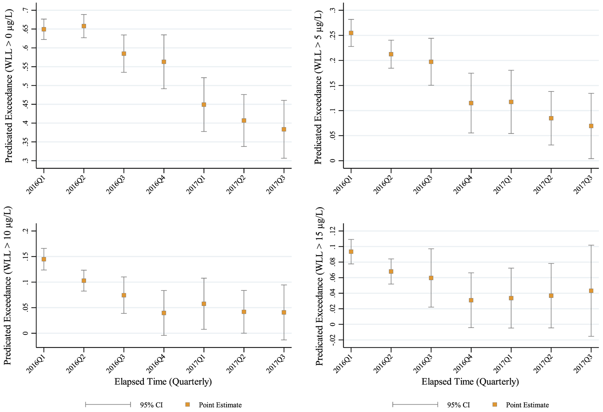
3.3. Leaded versus non-leaded service lines in time

Across all threshold models in Table 3, we find that the risk of exceedance declines with every week of elapsed time from the point of switchback to Detroit water. The decline in WLL exposure risk in time indicates steady improvement in OCCT practices in Flint’s community water system. Fig. 2 reinforces this observation of declining risk by showing predicted probabilities of WLL exceedance for various thresholds in time for leaded (LSL) versus galvanized (GSL), and other material service lines.

Fig. 2.

Predicted Probabilities of Water Lead Threshold Exceedance by Leaded versus Galvanized Steel versus Other Material Service Lines by Elapsed Time since Switchback to Detroit Water. Predicted probabilities are derived by estimating Eq. (1): $WL{L}_{ijt}=X_{\mathit{i}\mathit{j}\mathit{t}}\mathit{\beta }{+}_i+{\epsilon }_{it}={\beta }_0+{\beta }_1\sqrt{E{L}_{ijt}}+{\beta }_2{L}_{ij}+{\beta }_3{G}_{ij}+{\mathrm{\Gamma }}_1{C}_{ijt}+{\mathrm{\Gamma }}_2{B}_{ijt}+{\mathrm{\Gamma }}_3{K}_{ijt}+{\mathrm{\Gamma }}_4{T}_i+{\mathrm{\Gamma }}_5{M}_{it}+{\theta }_i+{\epsilon }_{ijt}$. All other model covariates are fixed at sample means in the post-estimation of predicted probabilities.

Across all threshold models (WLL > 0, 5, 10 and 15 μg/L), we find that homes with leaded, galvanized steel and other service lines experience substantial reductions in risk of exceedance with the elapsed time since switchback to Detroit water. The differential risks of exceedance for leaded versus galvanized versus other material service lines over time converge more strongly as the threshold level increases. Importantly, as we drift toward the present, observed differences in the risk of exceedance among homes with leaded versus non-leaded service lines are indistinguishable from chance. In fact, by 90 weeks from the date of switchback, the 95% confidence interval of the predicted probabilities of exceedance for water samples taken from homes with leaded service lines overlap the predicted probabilities for homes with galvanized and other material service lines for all thresholds but WLL > 0. More specific, by 90 weeks, the predicted probability of exceeding the LCR threshold of 15 μg Pb/L was 0.035, 0.032, and 0.025 for the leaded, galvanized steel, and other material service line homes, respectively.

3.4. Robustness

With the exception of WLL > 15 μg/L, across GEE models reported in Table 3 we find that threshold exceedance risk is significantly higher for homes with leaded service lines, and that threshold exceedance risk decreases in time from the point of switchback to Detroit water. As shown in Appendix Table 1, the decrease in threshold exceedance in time obtains with restriction of analysis to only homes observed in both Sentinel waves with leaded service lines. In Appendix Table 2, showing the odds of water lead threshold exceedance stratified by Sentinel sampling wave, we find that the amplification effect of a leaded service line is pronounced in Wave I versus Wave II. In fact, in Wave II, as compared to the reference group of other service line material type, homes with leaded service lines have comparable risk of a water sample eclipsing 5, 10, and 15 μg/L. In Appendix Table 3, we report odds ratios of water lead threshold exceedance with different elapsed time functions or g (). Results pertaining to untransformed and natural log transformation of elapsed time from Flint’s switchback to Detroit water behave similarly to the square root operation of time shown in Table 3. Finally, Appendix Table 4 shows odds ratios of water lead threshold exceedance with various reference group definitions. In Reference I models, the reference group of service line material type excludes homes classified as “unknown.” In Reference II models, the reference group of service line material type excludes homes classified as “unknown” and “plastic” leaving only homes with “copper” service lines. Whatever the definition of the reference group, we find that threshold exceedance risk is significantly higher for homes with leaded service lines, and that exceedance risk declines in time from Flint’s switchback to Detroit water, with coefficients behaving near identically to what is reported in Table 3.

3.5. Discrete factor model results

Table 4 shows average partial effects from discrete factor models. As compared to the reference group of homes with other material service lines, results show that homes with leaded service lines are statistically significantly more likely to exceed thresholds of WLL > 0, 5, and 10 μg/L (where p < 0.10). Specifically, average partial effects indicate that the risk of exceedance is 0.290, 0.136, 0.053, and 0.02 points higher for homes with leaded services lines at WLL thresholds of 0, 5, 10, and 15, respectively. Results from discrete factor models behave similarly to GEE results.

Table 4.

Average partial effects of discrete factor model.

	WLL > 0 μg/L	WLL > 5 μg/L	WLL > 10 μg/L	WLL > 15 μg/L
Elapsed time (weekly)	−0.25*** (0.04)	−0.16*** (0.03)	−0.07** (0.03)	−0.02 (0.02)
Galvanized service line	0.10** (0.04)	0.07 (0.04)	0.06 (0.03)	0.04 (0.02)
Lead service line	0.29*** (0.08)	0.14*** (0.05)	0.05 (0.03)	0.02 (0.02)
Water copper (μg/L)	0.17** (0.07)	0.14*** (0.04)	0.12*** (0.02)	0.07*** (0.02)
Bathroom	0.05 (0.04)	0.06 (0.04)	0.02 (0.03)	0.01 (0.02)
Kitchen	0.01 (0.04)	0.02 (0.036)	0.00 (0.03)	−0.01 (0.02)
Temperature (°F)	0.24*** (0.07)	0.15*** (0.05)	0.09*** (0.03)	0.02 (0.02)
Main break	0.00 (0.04)	0.03 (0.04)	0.02 (0.03)	0.02 (0.02)

Notes:

^**5% level,

^***1% level, two-sided tests; average temperature and water cooper concentration were divided by 100.

Recall, as shown in Fig. 1 summarizing results from GEE models, at WLL > 0 the difference between leaded and other material service lines was 0.27 points, at WLL > 5 the difference was 0.11 points, at WLL > 10 the difference was 0.05 points, and at WLL > 15 difference was 0.03 points. Results in Table 4 also show the reduction in the risk of exceedance of specified thresholds with elapsed time from the switchback to Detroit water. The coefficients reflect the absolute reduction in the probability exceedance for 100 weeks of elapsed time. Given unconditional means of 0.64, 0.244, and 0.125 for thresholds of WLL > 0, 5, and 10 μg/L, respectively, we find that at 100 weeks of elapsed time, probabilities of exceedance decrease significantly by 0.252, 0.156, and 0.064 points. For WLL > 15 μg/L, the observed reduction in the risk of exceedance is statistically insignificant.

3.6. Integrated exposure uptake biokinetic (IEUBK) model for lead in children

Child lead outcomes operate via multiple routes of exposure. In addition to lead exposure through drinking water – the focus of our investigation – lead can enter a child’s body through air, dust, and soil. With respect to air exposure, in the United States, deposition of lead-formulated aviation gasoline from piston-engine aircraft (PEA)⁹ accounts for the greatest fraction of atmospheric emissions (Zahran et al., 2017b). Another source of child lead exposure is lead-concentrated soils, primarily due to legacy deposition from lead-formulated automobile gasoline, dust from deteriorating or haphazardly removed lead-based paint, and historic point-source emissions. Contaminated soils¹⁰ enter a child’s body through ingestion (involving hand-to-mouth behaviors) or inhalation of lead-concentrated soil/dust re-suspended in summer months by turbulence (Filippelli et al., 2005; Laidlaw et al., 2005, Laidlaw and Filippelli, 2008, 2012; Zahran et al., 2010, 2011, 2013).

The IEUBK model for lead in children is a widely used simulation tool for estimating age-specific lead uptake (μg/day) and blood lead levels (μg/dL) as a function of these multiple channels of lead exposure (i.e., air, dietary, soil/dust, maternal, and water). The model has been extensively evaluated in terms of the adequacy of parameter estimates linking sources of lead exposure to the quantity of lead absorbed per unit of time and to the biokinetic movement of lead through the body and excretion pathways. IEUBK parameters are calibrated against empirical observation, and updated routinely as accumulated scientific evidence warrants adjustment of model elasticities. Of interest to this study is water lead exposure. In the arithmetic of the IEUBK model, the intake rate (IN) of leaded water is: IN_water = C_water × IR_water, where C is the water lead concentration and IR is the age-dependent water consumption or ingestion rate.

To derive the water lead concentration across Sentinel sampled homes j in period t, we re-estimate our GEE regression where water lead is measured as a continuous variable (μg/L). We generate two WLL (μg/L) predictions at 16 weeks and 90 weeks of elapsed time for each service-line material type (lead, galvanized steel, and other material), corresponding to the beginning and end of the Sentinel sampling effort, respectively. Six predictions were generated¹¹ in all. Given our interest in between-service line material types, IEUBK default parameters with respect to all other media of exposure (i.e., air, dietary, soil/dust, and maternal), bioavailability/absorption fractions, and water consumption (L/day) by age of child (USEPA 2007) are used. Predictions assume an absence of risk mitigation behavior (e.g. application of point-of-use filters, and bottled water consumption) and indifferent response by households with different service line material types.¹² Fig. 3 graphs expected water lead uptake and blood lead results by child age and by material of service line.

Fig. 3.

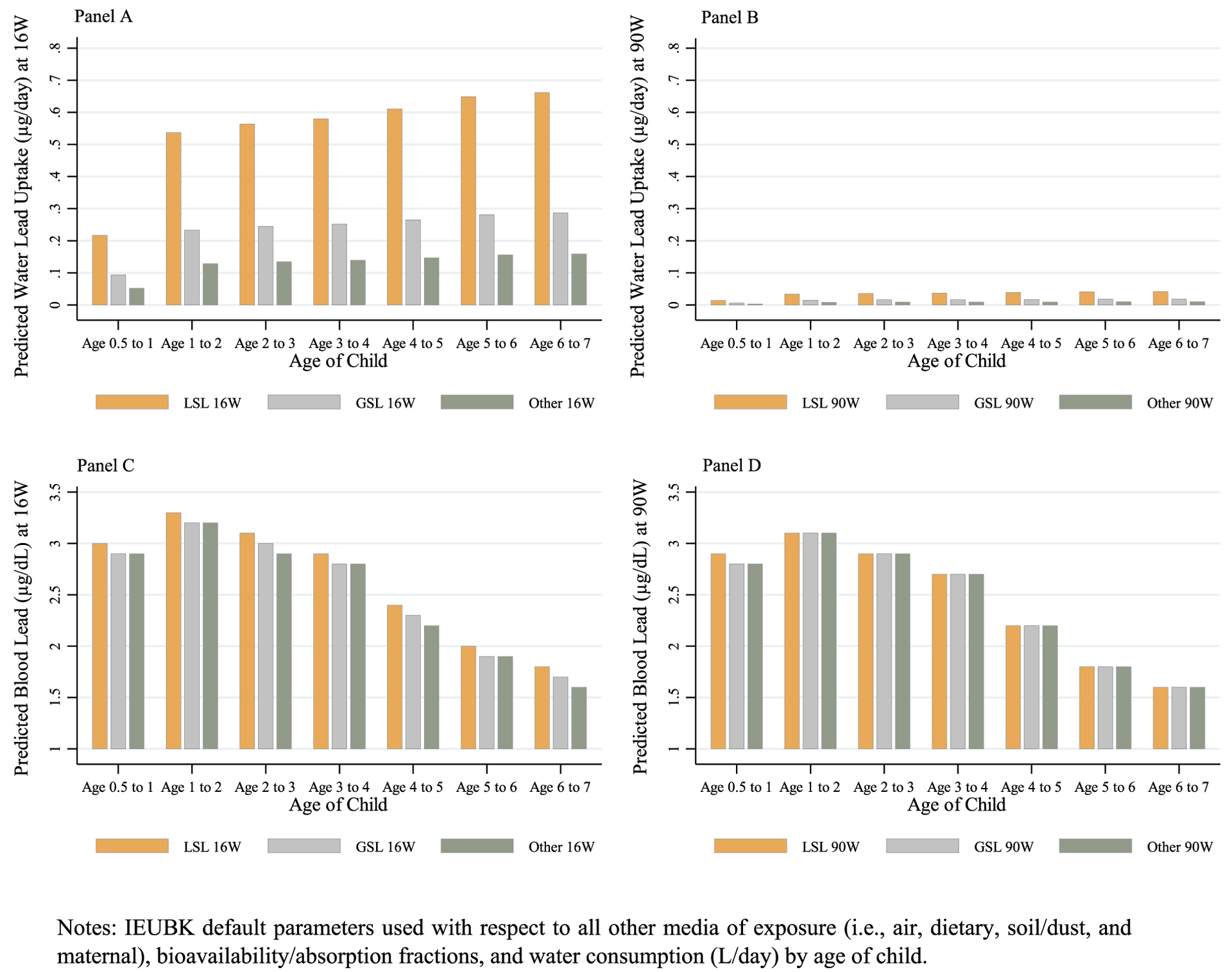
Integrated Exposure Uptake Biokinetic (IEUBK) Model for Lead in Children Simulations† at 16 and 90 Weeks of Elapsed Time from Switchback Notes: IEUBK default parameters used with respect to all other media of exposure (i.e., air, dietary, soil/dust, and maternal), bioavailability/absorption fractions, and water consumption (L/day) by age of child.

Starting with Panel A, at 16 weeks following the switchback in water source, we observe discernible differences in the expected lead uptake (μg/day) of children by service line material type. At 16 weeks, children residing in homes with leaded service lines were predicted to have consumed 4.5 and 2.5 times more lead per day than children residing in homes with other material and galvanized steel service lines, respectively. These differences in daily uptake by service line material type translate into differences is estimated blood lead levels in children by age. In Panel C (reflecting conditions at 16 weeks), children residing in homes with leaded service lines have higher estimated blood lead levels (μg/dL) across all age groups. As compared to children residing in homes with galvanized steel or other material service lines, children in homes with lead service lines have projected BLLs at 16 weeks that are 3.13%–5.88% and 3.13%–12.5% higher respectively, depending on the age of the child.

A different story obtains at 90 weeks after the switchback in water source. At 90 weeks (Panel B), the expected daily lead uptake of children residing in homes with lead service lines decreased 93% from the estimated daily uptake at 16 weeks. At 90 weeks, the quantity of water lead consumed by children in homes with lead service lines approaches zero, ranging from 0.016 to 0.048 μg/day, depending on the age of the child. The absolute difference in lead uptake for 6-year-old children in homes with leaded versus other material service lines decreases from 0.42 μg/day at 16 weeks to 0.010 μg/day at 90 weeks. In Panel D, we see that the sizeable reduction in daily lead uptake shown in Panel B near eliminates differences in expected BLLs of children residing in homes with lead versus galvanized steel and other material service lines. As compared with children residing in homes with galvanized steel or other material service lines, only children less than 1 year of age in homes with lead service lines have projected BLLs at 90 weeks that are one-tenth of 1 μg higher (2.9 vs 2.8 μg/dL). This reduction in the risk of elevated blood lead in children likely reflects improvements in OCCT in the Flint water system.

3.7. The social benefits of switching from lead to other material service lines

To quantify the significance of IEUBK simulation results, we estimate the annual cohort social benefits of switching from a lead to other material service line. To estimate the social benefits of LSLR, we use a standard syllogism in environmental health economics linking BLL to IQ point loss (Schwartz, 1994; Grosse et al., 2002; Gould, 2009). This syllogism is recommended in the EPAs Lead and Copper Rule Revisions White Paper, stating that LSLR replacement benefits ought to be estimated by the “avoided effects of lead exposure such as IQ loss in developing children” (USEPA 2016). However, it is important to note that additional health and human capital costs to children, adults, and broader society likely exist and are not incorporated in this narrow analysis recommended by the EPA.

Table 5 summarizes the steps involved in this social benefit calculation. Two series of calculations are performed, reflecting simulation results at 16 (Panel A) and 90 weeks (Panel B) of elapsed time from the return to Detroit water. In column (A) we estimate the count of at-risk children by age group calculated as the observed count of children in the 2010 decennial census multiplied by 0.52, reflecting the estimated count of parcels in need of partial or full replacement in Flint. Column (B) and (C) present estimated blood lead levels (BLL) for children residing in homes with leaded (LSL) and other material service lines (OMSL), respectively. BLLs are from IEUBK simulations with predicted WLLs from EQ. (3) of 2.304 μg/L for (B) and 0.552 μg/L for (C) at 16 weeks, and 0.147 μg/L for (B) and 0.035 μg/L for (C) at 90 weeks. Columns (D) and (E) show the expected loss of IQ points for children residing in homes with LSL and OMSL, respectively. For each service line type, IQ point loss is the product of the count of children, the corresponding estimated BLL and 0.513 (constituting the coefficient of IQ loss from a unit increase in BLL). The expected gain in IQ points for children (by age group) from switching a residential service line from LSL to OMSL (column F) is captured in the difference in IQ point loss in columns (E) and (D). By these calculations, we find that the social benefit of switching service line material type is substantial at 16 weeks (in terms of IQ points), and less so at 90 weeks from the switchback in Flint’s original water source.

Table 5.

The cohort social benefits of switch from lead to other material service lines (at 16 and 90 weeks from switchback).

Age Group	Count (A)	BLL for Lead Service Line (LSL) (B)	BLL for Other Material Service Line (OMSL) (C)	IQ Point Loss LSL (D)	IQ Point Loss OMSL (E)	IQ Point Gain from Switch of LSL to OMSL (F)
Panel A: 16 Weeks
.5 to 1 year	837	3	2.9	1288.14	1245.20	42.94
1–2 years	877	3.3	3.2	1484.67	1439.68	44.99
2–3 years	868	3.1	2.9	1380.38	1291.32	89.06
3–4 years	851	2.9	2.8	1266.03	1222.38	43.66
4–5 years	819	2.4	2.2	1008.35	924.32	84.03
5–6 years	830	2	1.9	851.58	809.00	42.58
6–7 years	795	1.8	1.6	734.10	652.54	81.57
Total
Panel B: 90 Weeks
.5 to 1 year	837	2.9	2.8	1245.20	1202.27	42.94
1–2 years	877	3.1	3.1	1394.69	1394.69	0.00
2–3 years	868	2.9	2.9	1291.32	1291.32	0.00
3–4 years	851	2.7	2.7	1178.72	1178.72	0.00
4–5 years	819	2.2	2.2	924.32	924.32	0.00
5–6 years	830	1.8	1.8	766.42	766.42	0.00
6–7 years	795	1.6	1.6	652.54	652.54	0.00

Notes: The estimated count of potentially affected children is in Column A, calculated as the observe count of children by age group in the 2010 Census multiplied by 0.52, reflecting the estimated count of parcels in need of partial or full replacement in Flint. Column B and C are derived from IEUBK simulations involving predicted WLLs of 2.304 μg/L for (B) and 0.552 μg/L for (C) at 16 weeks, and 0.147 μg/L for (B) and 0.035 μg/L for (C) at 90 weeks. Column D is the. Column D = A × B × 0.513 (reflecting IQ response from BLL dosage); Column E = A × C × 0.513. Column F = D – E.

4. Discussion and conclusion

Before discussing the potential lead reduction benefits of service line replacement efforts in Flint we recapitulate elements of research design and relevant findings. First, with respect to our outcome variable (WLL_ijt > Q), we pursued four different toxicological thresholds with Q increasing in stringency from > 15, to > 10, to > 5, and then to > 0 μgPb/L. Our choice to independently model four thresholds is because the LCR threshold of > 15 μg/L is not a health-based standard and is often mistakenly used to characterize risk of harm. In fact, the U.S. Centers for Disease Control and Prevention has stated repeatedly that there is no known safe level of lead exposure (U.S. CDC Advisory Committee, 2012; U.S. CDC Response to Advisory Committee, 2012; U.S. DHHS, 2012). Therefore, a non-zero quantity of lead in drinking water is cause for consideration.

With respect to findings, first, and over the observation period analyzed, we find statistically significant differences in the risk of water lead exposure across households with different service lines, with lead service lines more risky than galvanized steel and other material service lines (Tables 3 and 4, Fig. 1). With respect to the non-zero concentration outcome (> 0 μg/L), homes with leaded service lines are about 4x and 2x more likely to eclipse this threshold than homes with other material and galvanized steel service lines, respectively. Second, the risk of water lead exposure declined discernably in time for all service line types (Tables 3 and 4, Fig. 2). This result is compatible with recently published research on the decline of lead in sewage biosolids (Roy et al., 2019). Third, the effect of the passage of time is most evident at lower thresholds (Tables 3 and 4, Fig. 2). Fourth, the risk of exceedance of WLL > 15 μg/L appears to be governed by factors other than service line material type, given statistically insignificant coefficients (where p < 0.05) for lead and galvanized steel service lines in both GEE and discrete factor models (in Tables 3 and 4). All these results obtain across statistical procedures, sample restrictions, stratification analyses, various operations of elapsed time from Flint’s switchback to Detroit water, and different definitions of our reference group of other service line material type.

IEUBK model results indicate that at 16 weeks from the switchback in water supply, water lead uptake of children residing in homes with lead service lines was sizeable, varying from 0.217 to 0.662 μg/day, depending on the age of the child. Second, at 16 weeks, children residing in homes with leaded service lines consumed 4.5 and 2.5 times more lead per day than children residing in homes with other material and galvanized steel service lines, respectively. Third, at 90 weeks from the switchback in water source, the quantity of water lead consumed by children in homes with lead service lines decreased 93%, ranging from 0.016 to 0.048 μg/day. Fourth, at 90 weeks, estimated differences in daily water lead uptake were negligible across homes with different service line material types (Fig. 3, Panels A & B).

IEUBK model results also indicate that the risk of child lead exposure in Flint is likely driven by sources other than water, regardless of the period observed. That is, the percent of child blood lead attributable to non-water sources like air and soil/dust is notably larger than water lead sources at both 16 and 90 weeks from Flint’s switchback to Detroit water (Fig. 3, Panels C & D). In fact, at 90 weeks from Flint’s switchback to Detroit water, only children less than 1 year of age in homes with leaded service lines had projected BLLs different from children in homes with galvanized steel or other service line material types (Fig. 3, Panel D).

Our exercise on the social benefits of lead service line replacement efforts in Flint (using the EPAs suggested water lead → blood lead → child IQ syllogism) indicate that such efforts are likely to deliver modest cohort benefits in the present. As the risk of water lead exposure decreased over the observation period, the size of the estimated cohort benefit from LSLR efforts correspondingly decreased (Table 5). While the social benefits of LSLR would increase with the inclusion of other health effects (such as health care costs, long-term psychiatric and behavioral disorders, and physiological impairments) and harm to other segments of the population (adolescents, adults, and elderly), results indicate that water lead exposure risk in Flint has declined in time with evidence of risk convergence across homes with different service lines.¹³

While these results might suggest that LSLR may not be the most effective means of mitigating lead exposure, there are a number of technical and ethical reasons to support the FAST start initiative in Flint. From a technical perspective, it is important to proceed with caution as we are limited by the data from which we can draw conclusions. The current LCR monitoring protocol (i.e. 1-liter samples following 6 h of stagnation) does not fully capture the extent of lead exposure and is confounded by uncontrolled variables (flow rates, stagnation time, water temperature, etc.). Additionally, our assessment of social cost is conservative as undefined effects beyond the loss of IQ points are likely, given that there is no known safe level of lead exposure. From an ethical perspective, thousands of service lines have already been replaced, conferring a benefit on remediated homes. At a minimum, the benefit conferred on remediated homes is equal to the cost of service line replacement. Suspending the FAST start initiative mid-stream would create a distributional inequity across already remediated and non-remediated homes. In addition to suffering health insults, the residents of Flint suffered an immeasurable stigma cost. In the popular imagination, Flint is synonymous with polluted drinking water and institutional malfeasance. Arguably, to recover the reputation of the city, to overcome the substantial costs of stigma, and to recover the trust of residents,¹⁴ Flint officials are probably wise to proceed with the already funded project. With the removal of the very last service line, Flint can assure all current and future residents that the risk of lead exposure from service lines has been eliminated.¹⁵

This assurance does not mean an end to lead exposure from water, as sources of risk may include in-house fixtures and other parts of the water system. Recall, our results (see Tables 3 and 4) show that the likelihood of a water sample exceeding 15 μg/L is statistically unrelated to whether the home has a lead service line. Finally, while the FAST start initiative can reduce risk of exposure to lower tolerances of lead in water, and can function to recover lost trust, it cannot guarantee an end to lead exposure, as other pervasive sources of exposure risk like air, soil/dust, and paint lead remain.

Flint’s experience may inform national and local policy. As has been noted, the EPA’s Lead and Copper Rule Revisions White Paper provides direction for an analysis of whether LSL replacement reduces a significant source of lead in a cost-effective manner. The Flint experience suggests that OCCT techniques are effective in reducing water lead levels, implying that LSL replacement may not be necessary (at least in the short run). The impact of changes in Flint’s water supply – from Detroit water to the Flint River and back to Detroit water – on water lead exposure also suggests that OCCT techniques’ ability to reduce water lead content depends on the technical competence of local water authorities. Corrosion control techniques applied during this study were not typical of a well-managed system¹⁶ as they were applied in response to a massive corrosion event atypical of similar sized municipal water distribution systems. Further, they were implemented on a strained system that was already in disrepair. As municipal water systems and infrastructure age throughout the country and exceed their design life, their performance may change in unpredictable ways. Understanding how these aged systems perform during disturbances, including routine disturbances that may be underappreciated, is an emerging challenge (Love et al., 2019) and one that will require increased technical competence of drinking water operators.

Appendix

Appendix Table 1.

Odds of Water Lead Threshold Exceedance, Sentinel Data (February 16, 2016 to July 21, 2017), Restricting to Homes with Lead Service Lines Sampled in Both Sentinel Waves

	WLL > 0 μg/L	WLL > 5 μg/L	WLL > 10 μg/L	WLL > 15 μg/L
	OR	OR	OR	OR
Elapsed time (weekly)	0.64*** [0.54, 0.76]	0.72*** [0.64, 0.82]	0.72*** [0.56, 0.92]	0.75 [0.55, 1.03]
Water copper (μg/L)	1.01*** [1.01, 1.01]	1.00** [1.00, 1.01]	1.01*** [1.00, 1.01]	1.01*** [1.01, 1.01]
Bathroom sample	1.65 [0.80, 3.40]	0.89 [0.59, 1.33]	0.94 [0.54, 1.63]	0.90 [0.44, 1.82]
Kitchen sample	1.23 [0.75, 2.00]	0.86 [0.61, 1.22]	0.66 [0.36, 1.21]	0.47** [0.22, 0.99]
Temperature (°F)	1.02*** [1.01, 1.03]	1.01 [1.00, 1.02]	1.02** [1.00, 1.03]	1.01 [0.99, 1.03]
Main break	0.80 [0.37, 1.71]	1.27 [0.75, 2.14]	2.04** [0.91, 4.54]	1.53 [0.60, 3.94]
Wald χ2	52.65	41.92	33.90	51.08
N	832	832	832	832
NHouseholds	94	94	94	94

Notes: 95% confidence intervals in braces, and standard errors

^***p < 0.01,

^**p < 0.05, calculated using Huber/White/sandwich estimator of variance.

Appendix Table 2.

Odds of Water Lead Threshold Exceedance, Stratified by Sentinel Sampling Waves

	Wave I WLL > 0 μg/L	Wave II WLL > 0 μg/L	Wave I WLL > 5 μg/L	Wave II WLL > 5 μg/L	Wave I WLL > 10 μg/L	Wave II WLL > 10 μg/L	Wave I WLL > 15 μg/L	Wave II WLL > 15 μg/L
	OR	OR	OR	OR	OR	OR	OR	OR
Elapsed time (weekly)	0.95 [0.75, 1.20]	0.67*** [0.61, 0.74]	0.68*** [0.51, 0.91]	0.76*** [0.69, 0.85]	0.60*** [0.41, 0.87]	0.86** [0.75, 0.98]	0.58** [0.35, 0.97]	0.97 [0.84, 1.12]
Galvanized service line	1.80*** [1.31, 2.48]	1.14 [0.56, 2.31]	1.25 [0.88, 1.78]	1.60 [0.81, 3.15]	1.12 [0.70, 1.78]	1.18 [0.45, 3.12]	1.21 [0.71, 2.05]	0.93 [0.28, 3.15]
Lead service line	5.09*** [3.42, 7.58]	3.04*** [1.81, 5.09]	3.06*** [2.08, 4.51]	1.17 [0.74, 1.74]	2.33*** [1.52, 3.59]	1.07 [0.66, 1.74]	2.30*** [1.41, 3.76]	0.78 [0.46, 1.32]
Water copper (μg/L)	1.01*** [1.01, 1.01]	1.01*** [1.01. 1.01]	1.01*** [1.00, 1.01]	1.00*** [1.00, 1.01]	1.01*** [1.01, 1.01]	1.01*** [1.01, 1.01]	1.01*** [1.01, 1.01]	1.01*** [1.00, 1.01]
Bathroom	1.29 [0.97, 1.70]	1.17 [0.78, 1.77]	1.27 [0.95, 1.70]	0.86 [0.57, 1.32]	1.35 [0.96, 1.91]	0.61 [0.36, 1.05]	1.33 [0.88, 2.01]	0.85 [0.47, 1.53]
Kitchen	0.96 [0.80, 1.16]	0.80 [0.59, 1.09]	0.98 [0.79, 1.22]	0.81 [0.63, 1.05]	1.00 [0.76, 1.32]	0.66** [0.46, 0.96]	0.81 [0.57, 1.16]	0.58** [0.36, 0.92]
Temperature (°F)	1.00 [0.99, 1.01]	1.00 [1.00, 1.01]	1.00 [0.99, 1.01]	1.00 [0.99, 1.01]	1.01 [1.00, 1.02]	1.01 [0.99, 1.03]	0.99 [0.98, 1.01]	1.01 [0.99, 1.03]
Main break	0.94 [0.79, 1.13]	0.63** [0.41, 0.97]	1.11 [0.28, 3.32]	1.32 [0.95, 1.84]	1.26 [0.97, 1.64]	1.27 [0.72, 2.22]	0.96 [0.68, 1.37]	1.56 [0.89, 2,72]
Wald χ2	103.33	115.19	88.20	78.14	76.12	50.21	75.71	32.22
N	3162	1527	3162	1527	3162	1527	3162	1527
NHouseholds	766	190	766	190	766	190	766	190

Notes: 95% confidence intervals in braces, and standard errors

^***p < 0.01,

^**p < 0.05, calculated using the Huber/White/sandwich estimator of variance.

Appendix Table 3.

Odds of Water Lead Threshold Exceedance with Different Elapsed Time Functions

	WLL > 0 μg/L	WLL > 5 μg/L	WLL > 10 μg/L	WLL > 15 μg/L	WLL > 0 μg/L	WLL > 5 μg/L	WLL > 10 μg/L	WLL > 15 μg/L
	OR	OR	OR	OR	OR	OR	OR	OR
Elapsed time (weekly)	0.98*** [0.98, 0.99]	0.98*** [0.96, 0.99]	0.97*** [0.95, 0.99]	0.98 [0.96, 1.00]
In Elapsed time (weekly)					0.43*** [0.34, 0.54]	0.33*** [0.21, 0.52]	0.28*** [0.13, 0.60]	0.36** [0.15, 0.89]
Galvanized service line	1.61*** [1.19, 2.18]	1.60** [1.00, 2.57]	1.51 [0.81, 2.83]	1.43 [0.76, 2.68]	1.62*** [1.20, 2.20]	1.58 [0.99, 2.53]	1.46 [0.78, 2.73]	1.39 [0.74, 2.61]
Lead service line	3.87*** [2.71, 5.53]	2.01*** [1.29, 3.13]	1.78** [1.06, 2.99]	1.63 [0.94, 2.85]	3.99*** [2.79, 5.70]	2.07*** [1.33, 3.21]	1.77** [1.07, 2.94]	1.65 [0.95, 2.86]
Water copper (μg/L)	1.01*** [1.01, 1.01]	1.01*** [1.00, 1.01]	1.01*** [1.01, 1.01]	1.01*** [1.01, 1.01]	1.01*** [1.01, 1.01]	1.01*** [1.00, 1.01]	1.01*** [1.01, 1.01]	1.01*** [1.01, 1.01]
Bathroom	1.25 [0.99, 1.57]	1.04 [0.79, 1.39]	0.99 [0.68, 1.43]	1.08 [0.71, 1.64]	1.26** [1.00, 1.58]	1.05 [0.79, 1.40]	0.99 [0.69, 1.43]	1.08 [0.71, 1.64]
Kitchen	0.90 [0.77, 1.06]	0.87 [0.72, 1.06]	0.80 [0.59, 1.09]	0.69** [0.48, 0.97]	0.91 [0.78, 1.06]	0.87 [0.72, 1.05]	0.80 [0.59, 1.08]	0.68** [0.48, 0.96]
Temperature (°F)	1.01*** [1.00, 1.01]	1.00 [0.99, 1.01]	1.00 [0.99, 1.01]	0.99 [0.98, 1.00]	1.01*** [1.01, 1.01]	1.00 [1.00, 1.01]	1.00 [0.99, 1.02]	1.00 [0.98, 1.01]
Main break	0.91 [0.78, 1.08]	1.23** [1.01, 1.50]	1.35** [1.01, 1.82]	1.29 [0.93, 1.79]	0.91 [0.77, 1.07]	1.23** [1.01, 1.49]	1.35** [1.01, 1.81]	1.28 [0.93, 1.79]
Wald χ2	161.30	105.37	90.45	80.06	160.95	111.36	95.26	82.19
N	4689	4689	4689	4689	4689	4689	4689	4689
NHouseholds	820	820	820	820	820	820	820	820

Notes: 95% confidence intervals in braces, and standard errors

^***p < 0.01,

^**p < 0.05, calculated using the Huber/White/sandwich estimator of variance.

Appendix Table 4.

Odds of Water Lead Threshold Exceedance with Different Reference Group Definitions

	Reference I WLL > 0 μg/L	Reference II WLL > 0 μg/L	Reference I WLL > 5 μg/L	Reference II WLL > 5 μg/L	Reference I WLL > 10 μg/L	Reference II WLL > 10 μg/L	Reference I WLL > 15 μg/L	Reference II WLL > 15 μg/L
	OR	OR	OR	OR	OR	OR	OR	OR
Elapsed time (weekly)	0.77*** [0.72, 0.83]	0.77*** [0.72, 0.83]	0.71*** [0.61, 0.83]	0.71*** [0.61, 0.83]	0.68*** [0.52, 0.89]	0.68*** [0.53, 0.89]	0.73 [0.54, 1.00]	0.74 [0.54, 1.00]
Galvanized service line	1.69*** [1.25, 2.28]	1.69*** [1.24, 2.28]	1.64** [1.02, 2.65]	1.64** [1.01, 2.62]	1.55 [0.81, 2.97]	1.55 [0.79, 2.91]	1.43 [0.75, 2.73]	1.39 [0.73, 2.63]
Lead service line	4.18*** [2.88, 6.07]	4.18*** [2.93, 6.23]	2.09*** [1.33, 3.30]	2.09*** [1.32, 3.31]	1.86** [1.09, 3.17]	1.86** [1.07, 3.13]	1.66 [0.93, 2.95]	1.62 [0.91, 2.88]
Water copper (μg/L)	1.01*** [1.01, 1.01]	1.01*** [1.01, 1.01]	1.01*** [1.00, 1.01]	1.01*** [1.00, 1.01]	1.01*** [1.01, 1.01]	1.01*** [1.01, 1.01]	1.01*** [1.01, 1.01]	1.01*** [1.01, 1.01]
Bathroom	1.27** [1.00, 1.60]	1.27** [1.00, 1.60]	0.99 [0.74, 1.33]	0.99 [0.72, 1.31]	0.98 [0.67, 1.44]	0.98 [0.66, 1.43]	1.02 [0.66, 1.58]	1.02 [0.66, 1.58]
Kitchen	0.93 [0.79, 1.09]	0.93 [0.79, 1.09]	0.87 [0.72, 1.05]	0.87 [0.72, 1.05]	0.79 [0.57, 1.09]	0.79 [0.57, 1.09]	0.66** [0.46, 0.94]	0.65** [0.46, 0.93]
Temperature (°F)	1.01*** [1.00, 1.01]	1.01*** [1.00, 1.01]	1.00 [1.00, 1.01]	1.00 [1.00, 1.01]	1.00 [0.99, 1.01]	1.00 [0.99, 1.01]	0.99 [0.98, 1.01]	0.99 [0.98, 1.01]
Main break	0.92 [0.78, 1.08]	0.92 [0.78, 1.09]	1.25** [1.03, 1.53]	1.25** [1.02, 1.52]	1.37** [1.01, 1.85]	1.37** [1.01, 1.86]	1.28 [0.91, 1.79]	1.28 [0.91, 1.79]
Wald χ2	157.08	163.46	104.49	104.01	92.43	92.41	77.63	73.81
N	4544	4516	4544	4516	4544	4516	4544	4516
NHouseholds	789	785	789	785	789	785	789	785

Notes: 95% confidence intervals in braces, and standard errors

^***p < 0.01,

^**p < 0.05,

calculated using the Huber/White/sandwich estimator of variance. In Reference I models, the reference group of service line material type excludes homes classified as “unknown.” In Reference II models, the reference group of service line material type excludes homes classified as “unknown” and “plastic” leaving only homes with “copper” service lines.

Appendix Fig. 1.

Predicted Probabilities of Threshold Exceedance with Year-Quarter Indicator Variables. Notes: Predicted probabilities are derived by estimating Eq. (2): $WL{L}_{ijt}=X_{\mathit{i}\mathit{j}\mathit{t}}\mathit{\beta }{+}_i+{\epsilon }_{it}={\beta }_0+{\beta }_{1}e{l}_{ijt}+{\beta }_2{L}_{ij}+{\beta }_3{G}_{ijt}+{\mathrm{\Gamma }}_2{B}_{ijt}+{\mathrm{\Gamma }}_2{K}_{ijt}+{\mathrm{\Gamma }}_4{T}_i+{\mathrm{\Gamma }}_5{M}_{jt}+{\theta }_i+{\epsilon }_{ij}$. el is an indicator variable that assumes a value of 1 if a water sample taken from household occurs in a specified year-quarter, and 0 otherwise. All other model covariates are fixed at sample means in the post-estimation of predicted probabilities.

Appendix Fig. 2.

Present-Period Projected Probabilities of Water Lead Threshold Exceedance by Leaded versus Galvanized Steel versus Other Materials Service Lines. Notes: The Sentinel II sampling effort suspended on July 21, 2017. As of May 6, 2018, the Flint water system benefitted (in terms of optimal corrosion control efforts) from an additional 41 weeks of elapsed time from the moment of water source switchback. Leveraging log odds across threshold models corresponding to leaded service lines, elapsed time, and water copper concentrations, we project into the present expected probabilities of exceedance across specified thresholds for leaded versus non-leaded service lines. Figure Appendix 2 shows expected risks of threshold exceedance for the first week of May 2018. Other things held equal, we project that a water sample taken from a home with a leaded service line is significantly more likely to record a non-zero WLL. The expected probability of non-zero exceedance is 0.491 for leaded service line samples, 0.280 for galvanized steel service lines, and 0.190 for other material service line samples. With respect to the projected risk of WLL > 5 μg/L, the expected probability is 0.053 for leaded service line samples, 0.040 for galvanized steel service lines, and 0.025 for other service line samples. At WLL > 10 and 15 μg/L, the projected risk of exceedance for leaded service line water samples in the present is 0.016 and 0.014, respectively. For galvanized steel and other service line samples, the projected risk of eclipsing the Federal standard of 15 μg/L is similarly approaching zero at 0.012 and 0.009, respectively.

Appendix Fig. 3.

Monthly Average Blood Lead Level of Children in Flint and Piston Engine Aircraft Traffic at FNT. Note: Piston engine aircraft operations is equal to the number of arrivals and departures.

References

- DEQ [Department of Environmental Quality], 2018. Lead and Copper Rule Revision Summary Available at:. Department of Environmental Quality, State of Michigan, Lansing, MI: Accessed on. https://www.michigan.gov/documents/deq/deq-dwmadcws-2018_Rule_Revision_Summary_631411_7.pdf, Accessed date: 25 February 2019. [Google Scholar]
- ORR [Office of Regulatory Reinvention], 2016. Gov. Rick Snyder: initial ‘sentinel site’ data reveals mostly low lead levels, concerns remain: plan for regular data distribution detailed. Available at: https://www.michigan.gov/som/0,4669,7-192-29701-377410-,00.html, Accessed date: 25 February 2019.
- ORR [Office of Regulatory Reinvention], 2017. REGULATORY IMPACT STATEMENT (RIS) and COST-BENEFIT ANALYSIS ORR 2017–008 EQ. Department of Environmental Quality, State of Michigan, Lansing, MI: Available at: http://dmbinternet.state.mi.us/DMB/ORRDocs/RIS/1684_2017-008EQ_ris.pdf, Accessed date: 31 July 2018. [Google Scholar]
- USEPA [U.S. Environmental Protection Agency], 2000. Lead and Copper Rule: Summary of Revisions, EPA 815-R-99–020 Office of Water. U.S. Environmental Protection Agency, Washington DC. [Google Scholar]
- USEPA [U.S. Environmental Protection Agency], 2007. User’s Guide for the Integrated Exposure Uptake Biokinetic Model for Lead in Children (IEUBK) Windows®, EPA 9285.7–42 Office of Superfund Remediation and Technology Innovation, US Environmental Protection Agency, Washington DC. [Google Scholar]
- USEPA [U.S. Environmental Protection Agency], 2010. Integrated Exposure Uptake Biokinetic Model for Lead in Children, Windows® Version (IEUBKwin v1.1 Build 11). US Environmental Protection Agency, Washington DC, February Available at: https://www.epa.gov/superfund/lead-superfund-sites-software-and-users-manuals#integrated, Accessed date: 1 August 2018. [Google Scholar]
- USEPA [U.S. Environmental Protection Agency], 2016. Lead and Copper Rule Revisions White Paper US Environmental Protection Agency, Office of Water, Washington, DC: October. Available at: https://www.epa.gov/sites/production/files/2016-10/documents/508_lcr_revisions_white_paper_final_10.26.16.pdf, Accessed date: 31 July 2018. [Google Scholar]
- Aldred J, 2013. Justifying precautionary policies: incommensurability and uncertainty. Ecol. Econ 96, 132–140. [Google Scholar]
- American Water Works Association, 2017. M58 Internal Corrosion Control in Water Distribution Systems, Second Addition American Water Works Association, pp. 207. [Google Scholar]
- Baghurst PA, McMichael AJ, Wigg NR, Vimpani GV, Robertson EF, Roberts RJ, et al. , 1992. Environmental exposure to lead and children’s intelligence at the age of seven years. The Port Pirie Cohort Study. N. Engl. J. Med 327, 1279–1284. [DOI] [PubMed] [Google Scholar]
- Bonde JP, Joffe M, Apostoli P, et al. , 2002. Sperm count and chromatin structure in men exposed to inorganic lead: lowest adverse effect levelsOccupational and Environ. Med 59, 234–242. [DOI] [PMC free article] [PubMed] [Google Scholar]
- Crowards TM, 1998. Safe minimum standards: costs and opportunities. Ecol. Econ 25 (3), 303–314. [Google Scholar]
- Ebert A, 2018. All Lead Water Lines to Be Replaced under New Michigan Plan (1) Environment & Energy Report, Bureau of National Affairs; June 14. Available at: https://www.bna.com/lead-water-lines-n73014476506/, Accessed date: 31 July 2018. [Google Scholar]
- Filippelli GM, Laidlaw MA, Latimer JC, Raftis R, 2005. Urban lead poisoning and medical geology: an unfinished story. GSA Today (Geol. Soc. Am.) 15 (1), 4–11. [Google Scholar]
- Gilleskie Donna B, Lutz Byron F, 2002. The impact of employer-provided health insurance on dynamic employment transitions. J. Hum. Resour 37, 129–162. [Google Scholar]
- Goovaerts P, 2017a. Monitoring the aftermath of Flint drinking water contamination crisis: another case of sampling bias? Sci. Total Environ 590, 139–153. [DOI] [PMC free article] [PubMed] [Google Scholar]
- Goovaerts P, 2017b. The drinking water contamination crisis in Flint: modeling temporal trends of lead level since returning to Detroit water system. Sci. Total Environ 581, 66–79. [DOI] [PMC free article] [PubMed] [Google Scholar]
- Gould E, 2009. Childhood lead poisoning: conservative estimates of the social and economic benefits of lead hazard control. Environ. Health Perspect 117 (7), 1162–1167. [DOI] [PMC free article] [PubMed] [Google Scholar]
- Grosse SD, Matte TD, Schwartz J, Jackson RJ, 2002. Economic gains resulting from the reduction in children’s exposure to lead in the United States. Environ. Health Perspect 110 (6), 563–569. [DOI] [PMC free article] [PubMed] [Google Scholar]
- Grossman DS, Slusky D, 2017. The Effect of an Increase in Lead in the Water System on Fertility and Birth Outcomes: the Case of Flint. West Virginia University College of Business and Economics Working Paper Series, Michigan, pp. 17–25. [Google Scholar]
- Hanna-Attisha M, LaChance J, Sadler RC, Champney Schnepp A, 2016. Elevated blood lead levels in children associated with the Flint drinking water crisis: a spatial analysis of risk and public health response. Am. J. Public Health 106 (2), 283–290. [DOI] [PMC free article] [PubMed] [Google Scholar]
- Heard-Garris NJ, Roche J, Carter P, Abir M, Walton M, Zimmerman M, Cunningham R, 2017. Voices from flint: community perceptions of the flint water crisis. J. Urban Health 94 (6), 776–779. [DOI] [PMC free article] [PubMed] [Google Scholar]
- Hubbard AE, AhernFleischer JNL, Van der Laan M, Lippman SA, Jewell N, Bruckner T, Satariano WA, 2010. To GEE or not to GEE: comparing population average and mixed models for estimating the associations between neighborhood risk factors and health. Epidemiology 21 (4), 467–474. [DOI] [PubMed] [Google Scholar]
- Ignasiak Z, Slawinska T, Rozek K, Little BB, Malina RM, 2006. Lead and growth status of school children living in the copper basin of south-western Poland: differential effects on bone growth. Ann. Hum. Biol 33 (4), 401–414. [DOI] [PubMed] [Google Scholar]
- Kessler R, 2013. Sunset for leaded aviation gasoline? Environ. Health Perspect 1212, A54–A57. [DOI] [PMC free article] [PubMed] [Google Scholar]
- Laidlaw MA, Filippelli GM, 2008. Resuspension of urban soils as a persistent source of lead poisoning in children: a review and new directions. Appl. Geochem 23 (8), 2021–2039. [Google Scholar]
- Laidlaw MA, Mielke HW, Filippelli GM, Johnson DL, Gonzales CR, 2005. Seasonality and children’s blood lead levels: developing a predictive model using climatic variables and blood lead data from Indianapolis, Indiana, Syracuse, New York, and New Orleans, Louisiana (USA). Environ. Health Perspect 113 (6), 793. [DOI] [PMC free article] [PubMed] [Google Scholar]
- Laidlaw MA, Zahran S, Mielke HW, Taylor MP, Filippelli GM, 2012. Re-suspension of lead contaminated urban soil as a dominant source of atmospheric lead in Birmingham, Chicago, Detroit and Pittsburgh, USA. Atmos. Environ 49, 302–310. [Google Scholar]
- Laidlaw MA, Filippelli GM, Sadler RC, Gonzales CR, Ball AS, Mielke HW, 2016. Children’s blood lead seasonality in flint, Michigan (USA), and soil-sourced lead hazard risks. Int. J. Environ. Res. Public Health 13 (4), 358. [DOI] [PMC free article] [PubMed] [Google Scholar]
- Lee RG, Becker WC, Collins DW, 1989. Lead at the tap: sources and control. J. Am. Water Works Assoc 81 (7), 52–62. [Google Scholar]
- Love NG, Gebrie GS, Adejumo HA, McElmurry SP, 2019. Drinking water infrastructure in shrinking and expanding cities: the impact on water quality and public health Magil G, Benedict J (Eds.), Cascading Challenges in the Global Water Crisis. Cambridge Scholars Publishing, Newcastle, UK: Chapter Three. [Google Scholar]
- Lytle DA, Schock MR, Triantafyllidou S, 2018. Identify lead plumbing sources to protect public health. Opflow 44 (3), 16–20. [Google Scholar]
- Masten SJ, Davies SH, Mcelmurry SP, 2016. Flint water crisis: what happened and why? J. Am. Water Works Assoc 108 (12), 22–34. [DOI] [PMC free article] [PubMed] [Google Scholar]
- Mielke HW, Zahran S, 2012. The urban rise and fall of air lead (Pb) and the latent surge and retreat of societal violence. Environ. Int 43, 48–55. [DOI] [PubMed] [Google Scholar]
- Moore K, 2016. Mayor weaver to kick off Fast start project with first lead line removal March 3. City of flint, flint, MI: Available at: https://www.cityofflint.com/2016/03/03/mayor-weaver-to-kick-off-fast-start-project-with-first-lead-line-removal/, Accessed date: 31 July 2018. [Google Scholar]
- Mroz TA, 1999. Discrete factor approximations in simultaneous equation models: estimating the impact of a dummy endogenous variable on a continuous outcome. J. Econom 92 (2), 233–274. [DOI] [PubMed] [Google Scholar]
- Olson TM, Wax M, Yonts J, Heidecorn K, Haig SJ, Yeoman D, Hayes Z, Raskin L, Ellis BR, 2017. Forensic estimates of lead release from lead service lines during the Water Crisis in Flint, Michigan. Environ. Sci. Technol. Lett 4 (9), 356–361. [Google Scholar]
- Pieper KJ, Tang M, Edwards MA, 2017. Flint water crisis caused by interrupted corrosion control: investigating “ground zero” home. Environ. Sci. Technol 51 (4), 2007–2014. [DOI] [PubMed] [Google Scholar]
- Response USCDC, 2012. Response to Advisory Committee on Childhood Lead Poisoning Prevention Recommendations in “Low Level Lead Exposure Harms Children: a Renewed Call of Primary Prevention”. http://www.cdc.gov/nceh/lead/acclpp/cdc_response_lead_exposure_recs.pdf, Accessed date: 15 March 2013.
- Roy S, Tang M, Edwards MA, 2019. Lead release to potable water during the Flint, Michigan water crisis as revealed by routine biosolids monitoring data. Water Res 160, 475–483. [DOI] [PubMed] [Google Scholar]
- Schwartz J, 1994. Social benefits of reducing lead exposure. Environ. Res 66, 105–124. [DOI] [PubMed] [Google Scholar]
- Schwartz J, 1995. Lead, blood pressure, and cardiovascular disease in men. Arch. Environ. Health 50 (1), 31–37. [DOI] [PubMed] [Google Scholar]
- USCDC Advisory Committee, 2012. Center for disease control, prevention’s advisory committee on childhood lead poisoning, prevention (ACCLPP). Low level lead exposure harms children: a renewed call for primary prevention. http://www.cdc.gov/nceh/lead/ACCLPP/Final_Document_010412.pdf, Accessed date: 15 March 2013. [Google Scholar]
- USDHHS (Department of Health and Human Sciences) Natl. Toxicol. Program Monogr. Health Eff. Low-Level Lead http://ntp.niehs.nih.gov/NTP/ohat/Lead/Final/MonographHealthEffectsLowLevelLead_Final_508.pdf, 2012. [Accessed 21 February 2013].
- Wooldridge JM, 2001. Econometric Analysis of Coss Section and Panel Data. MIT Press, Cambridge, Massachusetts. [Google Scholar]
- Wooldridge JM, 2010. Econometric Analysis of Cross Section and Panel Data, second ed. MIT Press, Cambridge, MA. [Google Scholar]
- Zahran S, Mielke HW, Gonzales CR, Powell ET, Weiler S, 2010. New Orleans before and after Hurricanes Katrina/Rita: a quasi-experiment of the association between soil lead and children’s blood lead. Environ. Sci. Technol 44 (12), 4433–4440. [DOI] [PubMed] [Google Scholar]
- Zahran S, Mielke HW, Weiler S, Gonzales CR, 2011. Nonlinear associations between blood lead in children, age of child, and quantity of soil lead in metropolitan New Orleans. Sci. Total Environ 409 (7), 1211–1218. [DOI] [PubMed] [Google Scholar]
- Zahran S, Laidlaw MA, McElmurry SP, Filippelli GM, Taylor M, 2013. Linking source and effect: resuspended soil lead, air lead, and children’s blood lead levels in Detroit, Michigan. Environ. Sci. Technol 47 (6), 2839–2845. [DOI] [PubMed] [Google Scholar]
- Zahran S, McElmurry SP, Sadler RC, 2017a. Four phases of the Flint water crisis: evidence from blood lead levels in children. Environ. Res 157, 160–172. [DOI] [PMC free article] [PubMed] [Google Scholar]
- Zahran S, Iverson T, McElmurry SP, Weiler S, 2017b. The effect of leaded aviation gasoline on blood lead in children. Journal of the Association of Environmental and Resource Economists 4 (2), 575–610. [Google Scholar]
- Zahran S, McElmurry SP, Kilgore PE, Mushinski D, Press J, Love NG, Sadler RC, Swanson MS, 2018. Assessment of the Legionnaires’ disease outbreak in flint, Michigan. Proc. Natl. Acad. Sci 115 (8), E1730–E1739. [DOI] [PMC free article] [PubMed] [Google Scholar]