Mathematical analysis of swine influenza epidemic model with optimal control

Abstract

A deterministic model is designed and used to analyze the transmission dynamics and the impact of antiviral drugs in controlling the spread of the 2009 swine influenza pandemic. In particular, the model considers the administration of the antiviral both as a preventive as well as a therapeutic agent. Rigorous analysis of the model reveals that its disease-free equilibrium is globally asymptotically stable under a condition involving the threshold quantity-reproduction number ${\mathcal{R}}_c$. The disease persists uniformly if ${\mathcal{R}}_c>1$ and the model has a unique endemic equilibrium under certain condition. The model undergoes backward bifurcation if the antiviral drugs are completely efficient. Uncertainty and sensitivity analysis is presented to identify and study the impact of critical model parameters on the reproduction number. A time dependent optimal treatment strategy is designed using Pontryagin’s maximum principle to minimize the treatment cost and the infected population. Finally the reproduction number is estimated for the influenza outbreak and model provides a reasonable fit to the observed swine (H1N1) pandemic data in Manitoba, Canada, in 2009.

Introduction

Influenza is a viral infection which is primarily transmitted through respiratory droplets produced by coughing and sneezing by an infected person [13, 41, 46]. Fever, cough, headache, muscle and joint pain, and reddened eyes are common symptoms of influenza. The infection, mostly prevalent in young children, elderly, pregnant women and patients with particular medical conditions such as chronic heart disease, has an initial incubation period of 1–4 days followed by a latency period of 2–10 days [33, 41, 46].

For the past few centuries, influenza remains a serious threat to public health around the globe [2, 13, 41, 46]. It is reported that an influenza epidemic might have occurred in the sixteenth century [38]. During the past century, thousands of people lost their lives during three disastrous pandemics which include the Spanish flu, Asian flu, and Hong Kong flu during the year 1918, 1958, and 1968 respectively [2, 38, 46]. Most recently in 2014, India had reported 937 cases and 218 deaths from swine flu. The reported cases and deaths in 2015 had surpassed the previous numbers. The total number of confirmed cases crossed 33,000 with death of more than 2000 [43].

In 2009, the world experienced the H1N1 influenza, also known as the Swine Influenza, an epidemic which led to over 16455 deaths globally [51], 25,828 confirmed cases [36] and 428 deaths [37] in Canada alone. In Canada, this epidemic occurred in two waves, first wave occurred during the spring of 2009 whereas the second wave started around early October 2009 [5] and spanned about 3 months as it diminished by the end of January 2010 [31]. It is believed that genetic re-assortment involving the swine influenza virus lineages might be the main factor behind the emergence of H1N1 pandemic [22]. Various behavioral factors and chronic health conditions are considered to impose an increased risk of infection severity among H1N1 individuals. In particular, pregnant women, especially in their third trimester and infants are at increased risk of hospitalization and intensive care unit (ICU) admission [8, 10, 23, 50]. Moreover, individuals with pre-existing chronic conditions such as asthma, chronic kidney and heart diseases, and obesity are at far greater risk of death and ICU admission in comparison to healthy individuals [11, 28]. Additionally, geographical location may also impart a great risk to the severity of the infection. It is observed that people residing in remote, isolated communities and aboriginals, in the Canadian province of Manitoba, experienced severe illness due to the pandemic H1N1 infections [45]. Most recent outbreak of 2014, in India, had reported 937 cases and 218 deaths from swine flu. The reported cases and deaths in 2015 had surpassed the previous numbers. The total number of confirmed cases crossed 33,000 with death of more than 2000 [43].

Like seasonal influenza, H1N1 influenza is also transmitted through coughing and sneezing by infected individuals. It may also be transmitted through contact with contaminated objects. Main symptoms of H1N1 infection include fever, cough, sore throat, body aches, headache, chills and fatigue [7]. Various preventive measures were taken to minimize H1N1 infection cases. These measures included (a) social exclusion such as closing schools during the epidemic and banning public gatherings etc., (b) mass vaccination mainly to high risk groups due to limited supply and (c) the use of antiviral drugs such as oseltamivir (Tamiflu) and zanamivir (Relenza) [6]. Although the epidemic breakout occurred in 2009, H1N1 influenza still poses significant challenges to public health worldwide [9, 14, 18, 47–49].

In view of the serious consequences posed by the H1N1 epidemic on the public health, various mathematical models have been proposed and analyzed in order to understand the transmission dynamics of the H1N1 influenza [3, 4, 17, 19, 21, 22, 34, 39]. In particular, Bo$\ddot{e}$lle et al. [3] estimated the basic reproduction number for the H1N1 influenza outbreak in Mexico. Gojovic et al. [19] proposed mitigation strategies to overcome H1N1 influenza. Sharomi et al. [39] presented an H1N1 influenza model that accounts for the role of an imperfect vaccine and antiviral drugs administered to infected individuals. In the past, the basic reproduction number ${\mathcal{R}}_c$ has also been calculated by various researchers to control the disease by considering most-sensitive parameters but these strategies were not time-dependent. Lenhart proposed HIV models [15, 27], using which time-dependent optimal controls were proposed. In this paper, we will propose an optimal treatment strategy to prevent the H1N1 influenza epidemic.

The purpose of the current study is to complement the aforementioned studies by formulating a new model in which the susceptible population is stratified according to the risk of infection. Our model also accounts for the impact of singular use of the antiviral drugs, administered as a preventive agents only i.e., given to susceptible individuals or, in addition, as a therapeutic agent i.e., given to individuals with symptoms of the pandemic H1N1 infection in the early stage of illness. In this study we will present a rigorous mathematical analysis of our model and show that our model, under suitable conditions involving the basic reproduction number ${\mathcal{R}}_c$, exhibits disease free equilibrium as well as the phenomenon of backward bifurcation. We will perform uncertainty and sensitivity analysis of ${\mathcal{R}}_c$ in order to identify crucial model parameters. Additionally we will also propose optimal strategies that will eliminate the infection with minimal application of resources.

The paper is organized as follows. The model is formulated in Sect. 2 and rigorously analyzed in Sect. 3. We perform uncertainty and sensitivity analysis in Sect. 4 and using ideas from optimal control theory, we present an optimal treatment strategy in Sects. 5 and 6 marks the end of our paper with a discussion on our results.

Model formulation

The total human population at time t, denoted by N(t), is sub-divided into nine mutually-exclusive sub-populations comprising of low risk susceptible individuals $\left(S_L(t)\right)$, high risk susceptible individuals $\left(S_H(t)\right)$, susceptible individuals who were given antiviral drugs/vaccines $\left(P(t)\right)$, latent individuals $\left(L(t)\right)$, symptomatic individuals at early stage $\left(I_1(t)\right)$, symptomatic individuals at later stage $\left(I_2(t)\right)$, hospitalized individuals $\left(H(t)\right)$, treated individuals $\left(T(t)\right)$ and recovered individuals $\left(R(t)\right)$, so that

$$\begin{array}{c}\hfill N(t)=S_L(t)+S_H(t)+P(t)+L(t)+I_1(t)+I_2(t)+H(t)+T(t)+R(t).\end{array}$$

The high risk susceptible population includes pregnant women, children, health-care workers and providers (including all front-line workers), the elderly and other immune-compromised individuals. The rest of the susceptible population is considered to be at low risk of acquiring H1N1 infection. The model to be considered in this study is given by the following deterministic system of non-linear differential equations (a schematic diagram of the model is given in Fig. 1, and the associated variables and parameters are described in Table 1).

$$\begin{array}{cc}\hfill \frac{d{S}_L}{dt}=& \mathit{\pi }(1-p)-\mathit{\lambda }{S}_L-{\mathit{\sigma }}_L{S}_L-\mathit{\mu }{S}_L,\hfill \\ \hfill \frac{d{S}_H}{dt}=& \mathit{\pi }p-{\mathit{\theta }}_H\mathit{\lambda }{S}_H-{\mathit{\sigma }}_H{S}_H-\mathit{\mu }{S}_H,\hfill \\ \hfill \frac{dP}{dt}=& {\mathit{\sigma }}_L{S}_L+{\mathit{\sigma }}_H{S}_H-{\mathit{\theta }}_P\mathit{\lambda }P-\mathit{\mu }P,\hfill \\ \hfill \frac{dL}{dt}=& \mathit{\lambda }(S_L+{\mathit{\theta }}_H{S}_H+{\mathit{\theta }}_{P}P)-(\mathit{\alpha }+\mathit{\mu })L,\hfill \\ \hfill \frac{d{I}_1}{dt}=& \mathit{\alpha }L-({\mathit{\tau }}_1+\mathit{\gamma }+\mathit{\mu })I_1,\hfill \\ \hfill \frac{d{I}_2}{dt}=& \mathit{\gamma }{I}_1-({\mathit{\tau }}_2+\mathit{\psi }+{\mathit{\varphi }}_{I_2}+\mathit{\mu }+\mathit{\delta })I_2,\hfill \\ \hfill \frac{dH}{dt}=& \mathit{\psi }{I}_2-({\mathit{\varphi }}_H+\mathit{\mu }+{\mathit{\theta }}_1\mathit{\delta })H,\hfill \\ \hfill \frac{dT}{dt}=& {\mathit{\tau }}_1{I}_1+{\mathit{\tau }}_2{I}_2-({\mathit{\varphi }}_T+\mathit{\mu })T,\hfill \\ \hfill \frac{dR}{dt}=& {\mathit{\varphi }}_{I_2}{I}_2+{\mathit{\varphi }}_{H}H+{\mathit{\varphi }}_{T}T-\mathit{\mu }R.\hfill \end{array}$$ 1

In (1), $\mathit{\pi }$ represents the recruitment rate into the population (all recruited individuals are assumed to be susceptible) and p is the fraction of recruited individuals who are at high risk of acquiring infection. Low risk susceptible individuals acquire infection at a rate $\mathit{\lambda }$, given by

$$\begin{array}{c}\hfill \mathit{\lambda }=\frac{\mathit{\beta }({\mathit{\eta }}_{1}L+I_1+{\mathit{\eta }}_2{I}_2+{\mathit{\eta }}_{3}H+{\mathit{\eta }}_{4}T)}{N},\end{array}$$

where $\mathit{\beta }$ is the effective contact rate, ${\mathit{\eta }}_i(i=1,\dots ,4)$ are the modification parameters accounting for relative infectiousness of individuals in the $L,I_2,H_1$ and T classes respectively in comparison to those in the $I_1$ class. High risk susceptible individuals acquire infection at a rate ${\mathit{\theta }}_H\mathit{\lambda }$, where ${\mathit{\theta }}_H>1$ accounts for the assumption that high risk susceptible individuals are more likely to get infected in comparison to low risk susceptible individuals. Low (high) risk susceptible individuals receive antiviral at a rate ${\mathit{\sigma }}_L$ (${\mathit{\sigma }}_H$), and individuals in all epidemiological classes suffer natural death at a rate $\mathit{\mu }$.

Fig. 1.

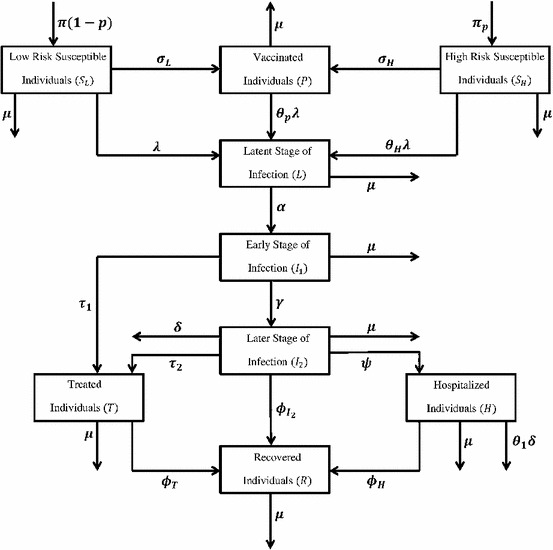
Schematic diagram of the model (1)

Table 1.

Description and nominal values of the model parameters

	Description	Value	Ref
$\mathit{\pi }$	Birth rate	1,119,583/80*365	Assumed
$1/\mathit{\mu }$	Average human lifespan	80*365	Assumed
p	Fraction of susceptible individuals at high risk for contracting infection	0.4	Assumed
$\mathit{\beta }$	Effective contact rate for transmitting H1N1 influenza	0.9 (initial)	To be estimated
${\mathit{\sigma }}_L$	Antiviral coverage rate for low risk susceptible individuals	0.3	[32]
${\mathit{\sigma }}_H$	Antiviral coverage rate for high risk susceptible individuals	0.5	[32]
$\mathit{\alpha }$	Rate at which latent individuals become infectious	1 / 1.9	[32]
${\mathit{\tau }}_1$	Treatment rate for individuals in the early stage of infection	1 / 5	[32]
${\mathit{\tau }}_2$	Treatment rate for individuals in the later stage of infection	1 / 3	[32]
${\mathit{\varphi }}_{I_2}$	Recovery rate for symptomatic infectious individuals in the	1/5	[32]
	Later stage
${\mathit{\varphi }}_H$	Recovery rate for hospitalized individuals	1/5	[32]
${\mathit{\varphi }}_T$	Recovery rate treated individuals	1/3	[32]
${\mathit{\eta }}_1$	Modification parameter (see text)	0.1	[32]
${\mathit{\eta }}_2$	Modification parameter (see text)	1/2	[32]
${\mathit{\eta }}_3$	Modification parameter (see text)	1.2	[32]
${\mathit{\eta }}_4$	Modification parameter (see text)	1	[32]
${\mathit{\theta }}_H$	Modification parameter for infection rate of high risk	1.2	[32]
	Susceptible individuals
$1-{\mathit{\theta }}_P$	Drug efficacy against infection	0.5	[32]
$\mathit{\psi }$	Hospitalization rate of individuals in $I_2$ class	0.5	[32]
$\mathit{\gamma }$	Progression rate from $I_1$ to $I_2$ classes	0.06	[32]
$\mathit{\delta }$	Disease-induced death rate of individuals in $I_2$ class	1/100	[32]
${\mathit{\theta }}_1\mathit{\delta }$	Disease-induced death rate for hospitalized individuals	1/100	[32]

Susceptible individuals who received prophylaxis $\left(P\right)$ can become infected at a reduced rate ${\mathit{\theta }}_P\mathit{\lambda }$, where $1-{\mathit{\theta }}_P\left(0<{\mathit{\theta }}_P<1\right)$ is the efficacy of the antiviral in preventing infection. Individuals in the latent class become infectious at a rate $\mathit{\alpha }$ and move to the symptomatic early stage of infection $I_1$. Individuals in the $I_1$ class receive antiviral treatment at a rate ${\mathit{\tau }}_1$. These individuals progress to the later infectious class ($I_2$) at a rate $\mathit{\gamma }$. Similarly, individuals in the $I_2$ class are treated (at a rate ${\mathit{\tau }}_2$), hospitalized (at a rate $\mathit{\psi }$), recover (at a rate ${\mathit{\varphi }}_{I_2}$) and suffer disease induced death (at a rate $\mathit{\delta }$). Hospitalized individuals, recover (at a rate ${\mathit{\varphi }}_H$) and suffer disease-induced death (at a reduced rate ${\mathit{\theta }}_1\mathit{\delta }$, where $0<{\mathit{\theta }}_1<1$ accounts for the assumption that hospitalized individuals, in the H class, are less likely to die than uncapitalized infectious individuals in the $I_2$ class).

Finally, treated individuals recover (at a rate ${\mathit{\varphi }}_T$). It is assumed that recovery confers permanent immunity against re-infection with H1N1. The model (1) is an extension of the model presented by Sharomi et al. [39] by:

• (i)administering antivirals to susceptible individuals.
• (ii)stratifying the susceptible population based on the risk of infection.

The basic qualitative properties of the model (1) will now be analyzed.

Basic properties of the model

Lemma 1

The closed set

$$\begin{array}{cc}\hfill \mathcal{D}=& \{(S_L,S_H,P,L,I_1,I_2,H,T,R)\in {\mathbb{R}}_{+}^9:N\le \frac{\mathit{\pi }}{\mathit{\mu }}\}\hfill \end{array}$$

is positively-invariant and attracting with respect to the model (1).

Thus, in the region $\mathcal{D}$, the model is well-posed epidemiologically and mathematically [20]. Hence, it is sufficient to study the qualitative dynamics of the model (1) in $\mathcal{D}$.

Existence and stability of equilibria

Local stability of disease-free equilibrium (DFE)

The model (1) has a DFE, given by

$$\begin{array}{cc}\hfill {\mathcal{E}}_0=& (S_L^{\ast },S_H^{\ast },P^{\ast },L^{\ast },I_1^{\ast },I_2^{\ast },H^{\ast },T^{\ast },R^{\ast })\hfill \\ \hfill =& \left(S_L^{\ast },S_H^{\ast },\frac{{\mathit{\sigma }}_L{S}_L^{\ast }+{\mathit{\sigma }}_H{S}_H^{\ast }}{\mathit{\mu }},0,0,0,0,0,0,\right),\hfill \end{array}$$

with,

$$\begin{array}{c}\hfill S_L^{\ast }=\frac{\mathit{\pi }(1-p)}{{\mathit{\sigma }}_L+\mathit{\mu }}\mathrm{and}{S}_H^{\ast }=\frac{\mathit{\pi }p}{{\mathit{\sigma }}_H+\mathit{\mu }}.\end{array}$$

Following [44], the linear stability of ${\mathcal{E}}_0$ can be established using the next generation operator method on system (1). The calculation is presented in Appendix. It follows that the control reproduction number, denoted by ${\mathcal{R}}_c$, is given by

$$\begin{array}{cc}\hfill {\mathcal{R}}_c& =\frac{\mathit{\beta }\mathit{\Omega }}{K_1}\{{\mathit{\eta }}_1+\frac{\mathit{\alpha }}{K_2}+\frac{{\mathit{\eta }}_4(\mathit{\alpha }\mathit{\gamma }{\mathit{\tau }}_2+\mathit{\alpha }{K}_3{\mathit{\tau }}_1)}{K_2{K}_3{K}_5}+\frac{\mathit{\alpha }\mathit{\gamma }{\mathit{\eta }}_2}{K_2{K}_3}+\frac{\mathit{\alpha }\mathit{\gamma }\mathit{\psi }{\mathit{\eta }}_3}{K_2{K}_3{K}_4}\}\hfill \end{array}$$ 2

where, $\mathit{\rho }$ is the spectral radius (dominant eigenvalue in magnitude) of the next generation matrix $F{V}^{-1}$ and $K_1=\mathit{\alpha }+\mathit{\mu },$ $K_2={\mathit{\tau }}_1+\mathit{\gamma }+\mathit{\mu },$ $K_3={\mathit{\tau }}_2+\mathit{\psi }+{\mathit{\varphi }}_2+\mathit{\mu }+\mathit{\delta },$ $K_4={\mathit{\psi }}_2+{\mathit{\varphi }}_3+\mathit{\mu }+{\mathit{\theta }}_1\mathit{\delta },$ $K_5={\mathit{\varphi }}_T+\mathit{\mu }.$ Hence, using Theorem 2 of [44], the following result is established.

The epidemiological significance of the control reproduction number, ${\mathcal{R}}_c$, which represents the average number of new cases generated by a primary infectious individual in a population where some susceptible individuals receive antiviral prophylaxis, is that the H1N1 pandemic can be effectively controlled if the use of antiviral can bring the threshold quantity $({\mathcal{R}}_c)$ to a value less than unity. Biologically-speaking, Lemma 2 implies that the H1N1 pandemic can be eliminated from the population (when ${\mathcal{R}}_c<1$) if the initial sizes of the sub-populations in various compartments of the model are in the basin of attraction of the DFE $({\mathcal{E}}_0)$. To ensure that disease elimination is independent of the initial sizes of the sub-populations of the model, it is necessary to show that the DFE is globally asymptotically stable (GAS). This is considered below, for a special case.

Lemma 2

The DFE, ${\mathcal{E}}_0,$ of the model (1), is locally asymptotically stable (LAS) if ${\mathcal{R}}_c<1$, and unstable if ${\mathcal{R}}_c>1$.

Global stability of DFE

The GAS property of ${\mathcal{E}}_0$ is presented here. We proved the following result: following:

Theorem 1

The DFE, ${\mathcal{E}}_0$, of the model (1) is GAS in $\mathcal{D}$ if ${\displaystyle {\mathcal{R}}_c\le R^{\ast }=\frac{\mathit{\Omega }}{{\mathit{\theta }}_H}}$ and ${\mathit{\theta }}_H=1$, ${\mathit{\theta }}_P=0.$

The proof is presented in the appendix.

Theorem 1 shows that the H1N1 pandemic can be eliminated from the community if the use of antivirals can lead to ${\mathcal{R}}_c\le R^{\ast }$.

Theorem 2

If ${\mathcal{R}}_c>1$, then the disease is uniformly persistent: there exists an $\mathit{ϵ}>0$ such that

$$\begin{array}{c}\hfill \underset{t\to \infty }{lim\; inf}\{L(t)+I_1(t)+I_2(t)+H(t)+T(t)\}>\mathit{ϵ}\end{array}$$

for all solutions $(S_L,S_H,P,L,I_1,I_2,H,T,R)$ of (1) with $L(0)+I_1(0)+I_2(0)+H(0)+T(0)>0$.

Proof is presented in the appendix. The epidemiological implication of the result is that disease will prevail in the community if ${\mathcal{R}}_c>1$.

It is convenient to define the following quantities

$$\begin{array}{c}\hfill \begin{array}{cc}\hfill {\mathcal{R}}_P& ={\mathcal{R}}_c{|}_{{\mathit{\tau }}_1={\mathit{\tau }}_2=0}=\frac{\mathit{\beta }\mathit{\Omega }}{K_1}\{{\mathit{\eta }}_1+\frac{\mathit{\alpha }}{K_2}+\frac{\mathit{\alpha }\mathit{\gamma }{\mathit{\eta }}_2}{K_2{K}_3}+\frac{\mathit{\alpha }\mathit{\gamma }\mathit{\psi }{\mathit{\eta }}_3}{K_2{K}_3{K}_4}\},\hfill \\ \hfill {\mathcal{R}}_T& ={\mathcal{R}}_c{|}_{{\mathit{\sigma }}_L={\mathit{\sigma }}_H=0}=\frac{\mathit{\beta }\mathit{\omega }}{K_1}\{{\mathit{\eta }}_1+\frac{\mathit{\alpha }}{K_2}+\frac{{\mathit{\eta }}_4(\mathit{\alpha }\mathit{\gamma }{\mathit{\tau }}_2+\mathit{\alpha }{K}_3{\mathit{\tau }}_1)}{K_2{K}_3{K}_5}+\frac{\mathit{\alpha }\mathit{\gamma }{\mathit{\eta }}_2}{K_2{K}_3}+\frac{\mathit{\alpha }\mathit{\gamma }\mathit{\psi }{\mathit{\eta }}_3}{K_2{K}_3{K}_4}\}\hfill \end{array}\end{array}$$ 3

where, $\mathit{\omega }=\mathit{\Omega }{|}_{{\mathit{\sigma }}_L={\mathit{\sigma }}_H=0}$. The quantities ${\mathcal{R}}_P$ and ${\mathcal{R}}_T$ represent the control reproduction numbers associated with the prophylactic (${\mathcal{R}}_P$) or therapeutic (${\mathcal{R}}_T$) use of antivirals in the community only.

Endemic equilibrium and backward bifurcation

In order to find endemic equilibria of the basic model (1) (that is, equilibria where atleast one of the infected components of the model (1) are non-zero), the following steps are taken. Let

$$\begin{array}{c}\hfill E_1=(S_L^{\ast \ast },S_H^{\ast \ast },P^{\ast \ast },L^{\ast \ast },I_1^{\ast \ast },I_2^{\ast \ast },H^{\ast \ast },T^{\ast \ast },R^{\ast \ast })\end{array}$$

represents an arbitrary endemic equilibrium of the model (1). Further, let

$$\begin{array}{c}\hfill {\mathit{\lambda }}^{\ast \ast }=\frac{\mathit{\beta }({\mathit{\eta }}_1{L}^{\ast \ast }+I_1^{\ast \ast }+{\mathit{\eta }}_3{I}_2^{\ast \ast }+{\mathit{\eta }}_4{H}_1^{\ast \ast }+{\mathit{\eta }}_6{T}^{\ast \ast })}{N^{\ast \ast }},\end{array}$$

be the associated force of infection at steady-state. Solving the equations of the model at steady-state yields:

$$\begin{array}{c}\hfill \begin{array}{cc}\hfill S_L^{\ast \ast }& =\frac{\mathit{\pi }(1-p)}{{\mathit{\lambda }}^{\ast \ast }+{\mathit{\sigma }}_L+\mathit{\mu }}\hfill \\ \hfill S_H^{\ast \ast }& =\frac{\mathit{\pi }p}{{\mathit{\theta }}_H{\mathit{\lambda }}^{\ast \ast }+{\mathit{\sigma }}_H+\mathit{\mu }}\hfill \\ \hfill P^{\ast \ast }& =\frac{{\mathit{\sigma }}_L{S}_L^{\ast \ast }+{\mathit{\sigma }}_H{S}_H^{\ast \ast }}{{\mathit{\theta }}_P{\mathit{\lambda }}^{\ast \ast }+\mathit{\mu }}=\frac{\mathit{\pi }(A{\mathit{\lambda }}^{\ast \ast }+B)}{Q}\hfill \\ \hfill L^{\ast \ast }& =\frac{{\mathit{\lambda }}^{\ast \ast }(S_L^{\ast \ast }+{\mathit{\theta }}_H{S}_H^{\ast \ast }+{\mathit{\theta }}_P{P}^{\ast \ast })}{K_1}=\frac{{\mathit{\lambda }}^{\ast \ast }(F{{\mathit{\lambda }}^2}^{\ast \ast }+G{\mathit{\lambda }}^{\ast \ast }+H)}{K_{1}Q}\hfill \\ \hfill I_1^{\ast \ast }& =\frac{\mathit{\alpha }}{K_2}{L}^{\ast \ast }=\frac{\mathit{\alpha }{\mathit{\lambda }}^{\ast \ast }(F{{\mathit{\lambda }}^2}^{\ast \ast }+G{\mathit{\lambda }}^{\ast \ast }+H)}{K_1{K}_{2}Q}\hfill \\ \hfill I_2^{\ast \ast }& =\frac{\mathit{\gamma }}{K_3}{I}_1^{\ast \ast }=\frac{\mathit{\gamma }\mathit{\alpha }{\mathit{\lambda }}^{\ast \ast }(F{{\mathit{\lambda }}^2}^{\ast \ast }+G{\mathit{\lambda }}^{\ast \ast }+H)}{K_1{K}_2{K}_{3}Q}\hfill \\ \hfill H^{\ast \ast }& =\frac{\mathit{\psi }}{K_4}{I}_2^{\ast \ast }=\frac{\mathit{\psi }\mathit{\gamma }\mathit{\alpha }{\mathit{\lambda }}^{\ast \ast }(F{{\mathit{\lambda }}^2}^{\ast \ast }+G{\mathit{\lambda }}^{\ast \ast }+H)}{K_1{K}_2{K}_3{K}_{4}Q}\hfill \\ \hfill T^{\ast \ast }& =\frac{{\mathit{\tau }}_1{I}_1^{\ast \ast }+{\mathit{\tau }}_2{I}_2^{\ast \ast }}{K_5}=\frac{{\mathit{\tau }}_1\mathit{\alpha }{\mathit{\lambda }}^{\ast \ast }(F{{\mathit{\lambda }}^2}^{\ast \ast }+G{\mathit{\lambda }}^{\ast \ast }+H)}{K_1{K}_2{K}_{5}Q}\hfill \\ \hfill & +\frac{{\mathit{\tau }}_2\mathit{\gamma }\mathit{\alpha }{\mathit{\lambda }}^{\ast \ast }(F{{\mathit{\lambda }}^2}^{\ast \ast }+G{\mathit{\lambda }}^{\ast \ast }+H)}{K_1{K}_2{K}_3{K}_{5}Q}\hfill \\ \hfill R^{\ast \ast }& =\frac{{\mathit{\varphi }}_{I_2}{I}_2^{\ast \ast }+{\mathit{\varphi }}_H{H}^{\ast \ast }+{\mathit{\varphi }}_T{T}^{\ast \ast }}{\mathit{\mu }}=\frac{{\mathit{\varphi }}_{I_2}\mathit{\gamma }\mathit{\alpha }{\mathit{\lambda }}^{\ast \ast }(F{{\mathit{\lambda }}^2}^{\ast \ast }+G{\mathit{\lambda }}^{\ast \ast }+H)}{\mathit{\mu }{K}_1{K}_2{K}_{3}Q}\hfill \\ \hfill & +\frac{{\mathit{\varphi }}_H\mathit{\psi }\mathit{\gamma }\mathit{\alpha }{\mathit{\lambda }}^{\ast \ast }(F{{\mathit{\lambda }}^2}^{\ast \ast }+G{\mathit{\lambda }}^{\ast \ast }+H)}{\mathit{\mu }{K}_1{K}_2{K}_3{K}_{4}Q}\hfill \\ \hfill & +\frac{{\mathit{\varphi }}_T{\mathit{\tau }}_1\mathit{\alpha }{\mathit{\lambda }}^{\ast \ast }(F{{\mathit{\lambda }}^2}^{\ast \ast }+G{\mathit{\lambda }}^{\ast \ast }+H)}{\mathit{\mu }{K}_1{K}_2{K}_{5}Q}+\frac{{\mathit{\varphi }}_T{\mathit{\tau }}_2\mathit{\gamma }\mathit{\alpha }{\mathit{\lambda }}^{\ast \ast }(F{{\mathit{\lambda }}^2}^{\ast \ast }+G{\mathit{\lambda }}^{\ast \ast }+H)}{\mathit{\mu }{K}_1{K}_2{K}_3{K}_{5}Q}.\hfill \end{array}\end{array}$$ 4

Using (8) and the expression for ${\mathit{\lambda }}^{\ast \ast }$ we get

$$\begin{array}{c}\hfill a_0{({\mathit{\lambda }}^{\ast \ast })}^3+b_0{({\mathit{\lambda }}^{\ast \ast })}^2+c_0({\mathit{\lambda }}^{\ast \ast })+d_0=0\end{array}$$ 5

where,

$$\begin{array}{cc}\hfill a_0& =A_1{A}_8\hfill \\ \hfill b_0& =A_6+A_2{A}_8-({\mathcal{R}}_c\mathit{\Omega })A_1\hfill \\ \hfill & =\mathit{\pi }{\mathit{\theta }}_H{\mathit{\theta }}_P(1-\frac{{\mathcal{R}}_c}{\mathit{\Omega }})+\mathit{\pi }p{\mathit{\theta }}_p(1-{\mathit{\theta }}_H)+A_2{A}_8\hfill \\ \hfill c_0& =A_4+A_3{A}_8-(\frac{{\mathcal{R}}_c}{\mathit{\Omega }})A_2\hfill \\ \hfill & =\mathit{\pi }(1-p)[{\mathit{\theta }}_P({\mathit{\sigma }}_H+\mathit{\mu })+\mathit{\mu }{\mathit{\theta }}_H](1-\frac{{\mathcal{R}}_c}{\mathit{\Omega }})\hfill \\ \hfill & +\mathit{\pi }p[\mathit{\mu }+{\mathit{\theta }}_P({\mathit{\sigma }}_L+\mathit{\mu })](1-\frac{{\mathit{\theta }}_H{\mathcal{R}}_c}{\mathit{\Omega }})+\mathit{\pi }{A}_7(1-\frac{{\mathit{\theta }}_P{\mathcal{R}}_c}{\mathit{\Omega }})+A_3{A}_8\hfill \\ \hfill d_0& =A_5-(\frac{{\mathcal{R}}_c}{\mathit{\Omega }})A_3\hfill \\ \hfill & =\mathit{\pi }\mathit{\mu }(1-p)({\mathit{\sigma }}_H+\mathit{\mu })[\mathit{\mu }(1-\frac{{\mathcal{R}}_c}{\mathit{\Omega }})+{\mathit{\sigma }}_L(1-\frac{{\mathit{\theta }}_P{\mathcal{R}}_c}{\mathit{\Omega }})]\hfill \\ \hfill & +\mathit{\pi }p\mathit{\mu }({\mathit{\sigma }}_L+\mathit{\mu })[\mathit{\mu }(1-\frac{{\mathit{\theta }}_H{\mathcal{R}}_c}{\mathit{\Omega }})+{\mathit{\sigma }}_L(1-\frac{{\mathit{\theta }}_P{\mathcal{R}}_c}{\mathit{\Omega }})]\hfill \end{array}$$

The large number of new coefficients ($A_i$) are defined in the Appendix.

The positive endemic equilibria of the model (1) are obtained by solving the cubic (5) for ${\mathit{\lambda }}^{\ast \ast }$ and substituting the results (positive values of ${\mathit{\lambda }}^{\ast \ast }$) into (4). The coefficient $a_0$, of (5), is always positive, and the signs of the remaining parameters are dependent upon the value of ${\mathcal{R}}_c$. Since we have a cubic equation to solve, it might not be possible to capture the dynamics of the system in general. Therefore, we will try to make natural and reasonable assumptions to study the system. Now we will discuss the solutions of (5) under different conditions.

Theorem 3

If ${\displaystyle \frac{{\mathcal{R}}_c}{\mathit{\Omega }}>\frac{1}{{\mathit{\theta }}_P}}$, then the model (1) exhibits a unique endemic equilibrium. However in case of ${\displaystyle \frac{{\mathcal{R}}_c}{\mathit{\Omega }}<\frac{1}{{\mathit{\theta }}_H}}$ no endemic equilibrium exists.

Proof

If ${\displaystyle \frac{{\mathcal{R}}_c}{\mathit{\Omega }}<\frac{1}{{\mathit{\theta }}_H}}$, it is easy to verify that all the coefficients of (5) are positive. Therefore by Descartes’s sign rule there is no positive root and hence no endemic equilibrium.

However if ${\displaystyle \frac{{\mathcal{R}}_c}{\mathit{\Omega }}>\frac{1}{{\mathit{\theta }}_P}}$, we have $d_0<0$. Considering the other parameters, there is exactly one sign change among consecutive parameters. According to Descartes sign rule, we have exactly one positive root. Thus we have a unique endemic equilibrium. This completes the argument. $\square$

Now the question arises what happens when ${\displaystyle \frac{1}{{\mathit{\theta }}_H}<\frac{{\mathcal{R}}_c}{\mathit{\Omega }}<\frac{1}{{\mathit{\theta }}_P}}$. In general, we cannot make any comment about this scenario. However the numerical simulations (using actual parameter estimates) suggest that there is no endemic equilibrium for ${\displaystyle \frac{1}{{\mathit{\theta }}_H}<\frac{{\mathcal{R}}_c}{\mathit{\Omega }}<1}$ and there exists a unique endemic equilibrium when ${\displaystyle 1<\frac{{\mathcal{R}}_c}{\mathit{\Omega }}<\frac{1}{{\mathit{\theta }}_P}}$.

The most important case arises when we assume that vaccination was perfect $({\mathit{\theta }}_P=0)$ and that infection rate of high risk susceptibles is unity $({\mathit{\theta }}_H=1)$. These assumptions reduce (5) to a quadratic equation given below

$$\begin{array}{c}\hfill e_0{({\mathit{\lambda }}^{\ast \ast })}^2+f_0({\mathit{\lambda }}^{\ast \ast })+g_0=0\end{array}$$ 6

where,

$$\begin{array}{cc}\hfill e_0& =\mathit{\pi }\mathit{\mu }Z\hfill \\ \hfill f_0& =\mathit{\pi }({\mathit{\sigma }}_L(1-p)+{\mathit{\sigma }}_{H}p)+\mathit{\pi }\mathit{\mu }+\mathit{\pi }\mathit{\mu }[({\mathit{\sigma }}_H+\mathit{\mu })(1-p)+p({\mathit{\sigma }}_L+\mathit{\mu })]Z-\mathit{\pi }\frac{{\mathcal{R}}_c}{\mathit{\Omega }}\hfill \\ \hfill g_0& =\mathit{\mu }[({\mathit{\sigma }}_H+\mathit{\mu })(1-p)+p({\mathit{\sigma }}_L+\mathit{\mu })](1-\frac{{\mathcal{R}}_c}{\mathit{\Omega }})+\mathit{\pi }B\hfill \end{array}$$

Lemma 3

If ${\displaystyle \frac{{\mathcal{R}}_c}{\mathit{\Omega }}<1}$ (along with perfect vaccination, ${\mathit{\theta }}_P=0$ and infection rate of high risk susceptibles, relative to that of low risk susceptibles, unity ${\mathit{\theta }}_H=1)$, then Backward Bifurcation is observed.

Proof

Clearly $e_0>0$. Now if ${\displaystyle \frac{{\mathcal{R}}_c}{\mathit{\Omega }}<1}$, we have $g_0>0$. Thus, when ${\displaystyle \frac{{\mathcal{R}}_c}{\mathit{\Omega }}<1}$ and $f_0<0$, we have two positive roots and hence we have Backward Bifurcation. The actual parameter estimates clearly show this phenomenon (Fig. 2). $\square$

Fig. 2.

Backward bifurcation

Uncertainty and sensitivity analysis

This section attempts to discuss the possible means of uncertainty in the values of our model parameters and to quantify the results. In a deterministic model, uncertainty can be generated by only input (initial conditions, parameters) variation and model parameters are among the most important part of the input data. The input data, particularly parameter estimates, can be uncertain due to the lack of sophisticated measuring methods, error in collecting and interpreting data and natural variations. Therefore, in order to study this uncertainty we perform global uncertainty and sensitivity analysis on our model output.

Uncertainty analysis gives a qualitative measure of parameters which are critical in the model output. This analysis also presents the degree of confidence on the model parameters. The Latin hypercube sampling will be used to perform the uncertainty analysis on the model parameters presented in Table 1. On the other hand, sensitivity analysis presents a qualitative measure of important parameters and quantifies the impact of each parameter on the model output, keeping the other parameters constant. Sensitivity analysis comprises of calculating the Partial Rank Correlation Coefficient (PRCC). The rank correlation coefficient is a standard method of quantifying the degree of monotonicity between an input parameter and the model output.

So far the dynamics of the model are determined by the threshold quantity ${\mathcal{R}}_c$, which determines the prevalence of the disease and therefore we consider it as our model output. Both uncertainty and sensitivity analyses are performed on the model parameters as the input data and ${\mathcal{R}}_c$ as the model output. The parameter estimates and the assigned distributions are given in the Appendix.

The estimate of ${\mathcal{R}}_c$ from uncertainty analysis is 1.32 with 95 $\%$ CI (1.13, 1.81). The probability that ${\mathcal{R}}_c$ $>$ 1 is 99 $\%$. This suggests that H1N1 will get endemic under the assumed conditions. However, the time taken to reach that state could be different.

From the sensitivity analysis, it is apparent that most significant parameters to ${\mathcal{R}}_c$ are (the ones having PRCC value above 0.5 or below $-$0.5) $\mathit{\beta }$, ${\mathit{\tau }}_1$, ${\mathit{\varphi }}_T$ and ${\mathit{\eta }}_4$. This result implies that these parameters need to be estimated with utmost precision and accuracy in order to capture the transmission dynamics of H1N1 (Figs. 3, 4).

Fig. 3.

Uncertainty analysis

Fig. 4.

Sensitivity analysis

Optimal control

Optimal control theory has found use in making decisions involving epidemic and biological models. The desired results and performance of the control functions depend on the different situations. Lenhart’s HIV models [15, 27] used optimal control to design the treatment strategies. Lenhart [25] provides a very good example of deciding how to divide the efforts between two treatment strategies (case holding and case finding) of the two strain TB model. Yan [52] used an optimal isolation strategy to fight the SARS epidemic. In [24] Joshi formulated two control functions as coefficients of the ODE system representing treatment effects in a two drug regime in an HIV immunology model. The goal was to maximize the concentration of T cells while minimizing the toxic effects of the drug. The analytic and numerical results illustrated the level of two drugs to be used over the chosen time interval. The required balancing effect between two competing goals was well predicted by optimal control theory.

While formulating an optimal control problem, deciding how and where to introduce the control (through vaccination, drug treatment etc) in the system of differential equation is very important. The formulation of the optimal control problem must be a reasonable and practical representation of the situation to be considered. The form of the optimal control depends heavily on the system being analyzed and the objective functional to be optimized. We will consider a quadratic dependence on the control in the objective functional, this will be briefly justified when we discuss our formulation of the problem.

The existence and uniqueness of the optimal control in an optimality system can be established using the Lipchitz properties of the differential equations[16, 35]. For a detailed example, see the work of Lenhart [15, 16]. After establishing the existence and the uniqueness results, we can confidently continue to numerically solving the optimality system to get the desired optimal control.

Control theory for models defined as a system of differential equations was formulated by Pontryagin [35]. Since his time, the theory and its application have grown considerably in number. Pontryagin’s maximum principle is a technique to optimize the performance criterion, (mostly cost and efficiency functional) which depends on different control parameters. The control parameters introduced are mostly functions of time appearing as coefficients in the model. The technique involves reducing a problem in which an optimal function over an entire time domain is to be determined to a standard optimization problem. This is achieved by appending an adjoint system of differential equations (with terminal boundary conditions) to the original model (state system) of differential equations (with initial conditions). The adjoint functions behave very similar to Lagrange multipliers (appending constraints to the function of several variables to be maximized or minimized). The adjoint variables maximize or minimize the state variables with respect to the desired objective functional. The details of the necessary conditions for the adjoint and optimal controls are presented here [16, 26, 35]. For the application of these results see [15].

We will attempt to optimize the treatment rates ${\mathit{\tau }}_1$ and ${\mathit{\tau }}_2$ of our model (1). We aim to design an optimal treatment strategy that minimizes an objective functional taking into account both the cost and the number of infectious individuals. Let the treatment rates ${\mathit{\tau }}_1$ and ${\mathit{\tau }}_2$ be functions of time. The control set $\mathbf{V}$ is

$$\begin{array}{cc}\hfill \mathbf{V}=& \{{\mathit{\tau }}_1(t),{\mathit{\tau }}_2(t):a_1\le {\mathit{\tau }}_1(t)\le b_1,a_2\le {\mathit{\tau }}_2(t)\le b_2,0\hfill \\ \hfill & \le t\le T,{\mathit{\tau }}_1(t)\text{are}{\mathit{\tau }}_2(t)\text{are Lebesgue measurable}\}.\hfill \end{array}$$ 7

The goal is to minimize the cost function defined as

$$\begin{array}{c}\hfill J[{\mathit{\tau }}_1(t),{\mathit{\tau }}_2(t)]={\int }_0^T\left[X_{1}P+X_2{I}_1+X_3{I}_2+X_{4}H+\frac{1}{2}{W}_1{\mathit{\tau }}_1^2(t)+\frac{1}{2}{W}_2{\mathit{\tau }}_2^2(t)\right]dt\\ \hfill \end{array}$$ 8

This objective functional (performance criterion) involves the numbers of infected individuals as well as the cost of treatment. Since the total cost includes not only the consumption for every individual but also the cost of organization, management, and cooperation, a non-linear cost function seems to be the right choice. In this paper, a quadratic function is implemented for measuring the control cost by reference to literature in epidemics control [15, 25, 27, 52]. The coefficients $W_1$ and $W_2$ are balancing cost factors due to scales and importance of the cost part of the objective functional, $b_1$ and $b_2$ are the maximum attainable values of the control, $X_i$ is the positive constants to keep balance in the population size in each class. We attempt to find an optimal control pair $({\mathit{\tau }}_1^{\ast },{\mathit{\tau }}_2^{\ast })$ such that

$$\begin{array}{c}\hfill J[{\mathit{\tau }}_1^{\ast },{\mathit{\tau }}_2^{\ast }]=\underset{{\mathit{\tau }}_1,{\mathit{\tau }}_2\in V}{min}J[{\mathit{\tau }}_1,{\mathit{\tau }}_2]\end{array}$$

The existence of an optimal solution to the optimal control problem can be established by Theorem III.4.1 and its corresponding Corollary in [16]. The boundedness of solutions to the system (3.1) for the finite time interval is needed to establish these conditions and $\mathcal{D}$ satisfies it. Pontryagin’s maximum principle [35] provides the necessary conditions to be satisfied by the optimal vaccination v(t). As stated earlier this reduces the problem to one of minimizing point wise a Hamiltonian, H, with respect to v

$$\begin{array}{c}\hfill H=X_{1}P+X_2{I}_1+X_3{I}_2+X_{4}H+\frac{1}{2}{W}_1{\mathit{\tau }}_1^2(t)+\frac{1}{2}{W}_2{\mathit{\tau }}_2^2(t)+\sum _{i=1}^{i=9}{\mathit{\xi }}_i{k}_i\end{array}$$ 9

where $k_i$ represents the right hand side of the modified model’s ith differential equation. Using the Pontryagin’s maximum principle [35] and the optimal control existence result from [16], we have

Theorem 4

There exists a unique optimal pair ${\mathit{\tau }}_1^{\ast }(t),{\mathit{\tau }}_2^{\ast }(t)$ which minimizes J over $\mathbf{V}$. Also, there exists adjoint system of ${\mathit{\xi }}_i$’s such that

$$\begin{array}{cc}\hfill {\displaystyle \frac{d{\mathit{\xi }}_1}{dt}}& =(\mathit{\lambda }+{\mathit{\sigma }}_L+\mathit{\mu }){\mathit{\xi }}_1-{\mathit{\sigma }}_L{\mathit{\xi }}_3-\mathit{\lambda }{\mathit{\xi }}_4\hfill \\ \hfill {\displaystyle \frac{d{\mathit{\xi }}_2}{dt}}& =({\mathit{\theta }}_H\mathit{\lambda }+{\mathit{\sigma }}_H+\mathit{\mu }){\mathit{\xi }}_2-{\mathit{\sigma }}_H{\mathit{\xi }}_3-{\mathit{\theta }}_H\mathit{\lambda }{\mathit{\xi }}_4\hfill \\ \hfill {\displaystyle \frac{d{\mathit{\xi }}_3}{dt}}& =({\mathit{\theta }}_P\mathit{\lambda }+\mathit{\mu }){\mathit{\xi }}_3-{\mathit{\theta }}_P\mathit{\lambda }{\mathit{\xi }}_4-X_1\hfill \\ \hfill {\displaystyle \frac{d{\mathit{\xi }}_4}{dt}}& ={\displaystyle \frac{\mathit{\beta }}{N}}{\mathit{\eta }}_1{S}_L{\mathit{\xi }}_1+{\displaystyle \frac{\mathit{\beta }}{N}}{\mathit{\eta }}_1{\mathit{\theta }}_H{S}_H{\mathit{\xi }}_2-{\displaystyle \frac{\mathit{\beta }}{N}}{\mathit{\eta }}_1(S_L+{\mathit{\theta }}_H{S}_H+{\mathit{\theta }}_{p}P){\mathit{\xi }}_4+C_1{\mathit{\xi }}_4-\mathit{\alpha }{\mathit{\xi }}_5\hfill \\ \hfill {\displaystyle \frac{d{\mathit{\xi }}_5}{dt}}& ={\displaystyle \frac{\mathit{\beta }}{N}}{S}_L{\mathit{\xi }}_1+{\displaystyle \frac{\mathit{\beta }}{N}}{\mathit{\theta }}_H{S}_H{\mathit{\xi }}_2-{\displaystyle \frac{\mathit{\beta }}{N}}(S_L+{\mathit{\theta }}_H{S}_H+{\mathit{\theta }}_{P}P)x{i}_4\hfill \\ \hfill & +C_2{\mathit{\xi }}_5-\mathit{\gamma }{\mathit{\xi }}_6-{\mathit{\tau }}_1^{\ast }(t){\mathit{\xi }}_8-X_2\hfill \\ \hfill {\displaystyle \frac{d{\mathit{\xi }}_6}{dt}}& ={\displaystyle \frac{\mathit{\beta }}{N}}{\mathit{\eta }}_2{S}_L{\mathit{\xi }}_1+{\displaystyle \frac{\mathit{\beta }}{N}}{\mathit{\eta }}_2{\mathit{\theta }}_H{S}_H{\mathit{\xi }}_2-{\displaystyle \frac{\mathit{\beta }}{N}}{\mathit{\eta }}_2(S_L+{\mathit{\theta }}_H{S}_H+{\mathit{\theta }}_{P}P)x{i}_4\hfill \\ \hfill & +C_3{\mathit{\xi }}_6-\mathit{\psi }{\mathit{\xi }}_7-{\mathit{\tau }}_2^{\ast }(t){\mathit{\xi }}_8-{\mathit{\varphi }}_{I_2}{\mathit{\xi }}_9-X_3\hfill \\ \hfill {\displaystyle \frac{d{\mathit{\xi }}_7}{dt}}& ={\displaystyle \frac{\mathit{\beta }}{N}}{\mathit{\eta }}_3{S}_L{\mathit{\xi }}_1+{\displaystyle \frac{\mathit{\beta }}{N}}{\mathit{\eta }}_3{\mathit{\theta }}_H{S}_H{\mathit{\xi }}_2-{{\displaystyle \frac{\mathit{\beta }}{\mathit{\eta }}}}_{3}N(S_L+{\mathit{\theta }}_H{S}_H+{\mathit{\theta }}_{P}P)x{i}_4\hfill \\ \hfill & +C_4{\mathit{\xi }}_7-{\mathit{\varphi }}_H{\mathit{\xi }}_9-X_4\hfill \\ \hfill {\displaystyle \frac{d{\mathit{\xi }}_8}{dt}}& =C_5{\mathit{\xi }}_8-{\mathit{\varphi }}_T{\mathit{\xi }}_9\hfill \\ \hfill {\displaystyle \frac{d{\mathit{\xi }}_9}{dt}}& =\mathit{\mu }{\mathit{\xi }}_9\hfill \end{array}$$

where $C_1={\mathit{\alpha }}_1+\mathit{\mu },$     $C_2={\mathit{\tau }}_1^{\ast }(t)+\mathit{\gamma }+\mathit{\mu },$    $C_3={\mathit{\tau }}_2^{\ast }(t)+\mathit{\psi }+{\mathit{\varphi }}_{I_2}+\mathit{\mu }+\mathit{\delta },$    $C_4={\mathit{\psi }}_2+{\mathit{\varphi }}_3+\mathit{\mu }+{\mathit{\theta }}_1\mathit{\delta },$    $C_5={\mathit{\varphi }}_T+\mathit{\mu }$

The transversality condition gives

$$\begin{array}{c}\hfill {\mathit{\xi }}_i(t_f)=0.\end{array}$$

The vaccination control is characterized as

$$\begin{array}{c}\hfill {\mathit{\tau }}_1^{\ast }(t)=min[b_1,max(a_1,\frac{I_1({\mathit{\xi }}_5-{\mathit{\xi }}_8)}{W_1})]\end{array}$$ 10

$$\begin{array}{c}\hfill {\mathit{\tau }}_2^{\ast }(t)=min[b_2,max(a_2,\frac{I_2({\mathit{\xi }}_6-{\mathit{\xi }}_8)}{W_2})].\end{array}$$ 11

Proof

It is easy to verify that the integrand of J is convex with respect to ${\mathit{\tau }}_1$ and ${\mathit{\tau }}_2$. Also the solutions of the (1) are bounded as $N(t)\le {\displaystyle \frac{\mathrm{\Pi }}{\mathit{\mu }}}$ for all time. Also it is clear the state system (1) has the Lipschitz property with respect to the state variables. With these properties and using Corollary 4.1 of [16], we have the existence of the optimal control.

Since we have the existence of the optimal vaccination control. Using the Pontryagin’s maximum principle, we obtain

$$\begin{array}{cc}\hfill {\displaystyle \frac{d{\mathit{\xi }}_1}{dt}}& =-\frac{\mathit{\partial }H}{\mathit{\partial }{S}_L},{\mathit{\xi }}_1(t_f)=0\hfill \\ \hfill {\displaystyle \frac{d{\mathit{\xi }}_2}{dt}}& =-\frac{\mathit{\partial }H}{\mathit{\partial }{S}_H},{\mathit{\xi }}_2(t_f)=0\hfill \\ \hfill ...\\ \hfill {\displaystyle \frac{d{\mathit{\xi }}_9}{dt}}& =-\frac{\mathit{\partial }H}{\mathit{\partial }R},{\mathit{\xi }}_9(t_f)=0\hfill \\ \hfill \end{array}$$

evaluated at the optimal control, which results in the stated adjoint system . The optimality condition is

$$\begin{array}{cc}\hfill \frac{\mathit{\partial }H}{\mathit{\partial }{\mathit{\tau }}_1}{|}_{{\mathit{\tau }}_1^{\ast }}& =0\hfill \\ \hfill \frac{\mathit{\partial }H}{\mathit{\partial }{\mathit{\tau }}_2}{|}_{{\mathit{\tau }}_2^{\ast }}& =0.\hfill \end{array}$$

Therefore on the set $\{t:a_1<{\mathit{\tau }}_1^{\ast }(t)<b_1,a_2<{\mathit{\tau }}_2^{\ast }(t)<b_2\}$, we obtain

$$\begin{array}{c}\hfill {\mathit{\tau }}_1^{\ast }(t)=\frac{I_1({\mathit{\xi }}_5-{\mathit{\xi }}_8)}{W_1}\\ \hfill {\mathit{\tau }}_2^{\ast }(t)=\frac{I_2({\mathit{\xi }}_6-{\mathit{\xi }}_8)}{W_2}.\end{array}$$

Considering the bounds on ${\mathit{\tau }}_1$ and ${\mathit{\tau }}_2$, we have the characterizations of the optimal control as in (14) and (15). Clearly the state and the adjoint functions are bounded. Also it is easily verifiable that state system and adjoint system has Lipschitz structure with respect to the corresponding variables, from here we obtain the uniqueness of the optimal control for sufficiently small time T [16, 35]. The uniqueness of the optimal control pair follows from the uniqueness of the optimality system, which consists of (3.1) and (3.5), with characterizations (3.6). Note here the uniqueness of the optimal control is only for a certain length of time. This restriction on the length of the time interval arises due to the opposite time orientations of (3.1), and (3.5); the state system has initial conditions and the adjoint system has final conditions. For example see [15], this restriction is very common in control problems (see [27]). $\square$

The optimality system consisting of 9 state system of differential equations and an adjoint system differential equations with $S_L(0)=S_{L0},S_H(0)=S_{H0},P(0)=P_0,L(0)=L_0,I_1(0)=I_{10},I_2(0)=I_{20},H(0)=H_0,T(0)=T_0,R(0)=R_0.$ $(\square )$

Next, we discuss the numerical solutions of the optimality system and the corresponding optimal control pair. The optimal treatment strategy is obtained by solving the optimality system. An iterative scheme is used for solving the optimality system. We start to solve the state equations with a guess for the control pair $({\mathit{\tau }}_1,{\mathit{\tau }}_2)$, using a forward Runge–Kutta method. The adjoint functions have final time conditions. Because of this transversality conditions on the adjoint functions , the adjoint equations are solved by a backward Runge–Kutta method using the current iteration solution of the state equations. Then, the controls are updated by using a convex combination of the previous control and the value from the characterizations. This process is repeated and iteration is stopped if the values of unknowns at the previous iteration are very close to the ones at the present iteration.

The parameter values used have ${\mathcal{R}}_c>1$ when the model without control is considered. Thus the disease is not expected to die out without intervention strategies.

Figure 5 represents the control strategy to be employed for the optimal results. This control strategy minimizes both the cost and the infected population $(I_1+I_2)$. It is well understood that in order to eradicate an epidemic, a large fraction of infected population needs to be treated. Therefore, an upper bound of 0.7 was chosen for treatment control. The optimal controls remain at higher values initially and then steadily decreasing to 0. In fact, at the beginning of simulated time, the optimal control is staying at higher values in order to treat as many infected as possible to prevent the susceptible individuals from getting infected and epidemic to break out. The steadily decreasing of the v is determined by the balance between the cost of the infected individuals and the cost of the controls. Figure 6 shows the infected $(I_1+I_2)$population for the optimal control and constant control. It is easy to see that the optimal control is much more effective for reducing the number of infected individuals and decreasing the time-span of the epidemic. As normally expected, in the early phase of the epidemic breakouts, keeping the control at their upper bound will directly lead to the decreasing of the number of the infected people. Figure 7 shows the cost associated with the optimal and constant control strategy. It is clear the cost of optimal strategy is much less than the cost of constant strategy. Moreover Fig. 8 represents control strategies for different values of the effective contact rate $\mathit{\beta }$. It can be observed that increased effective contact rate requires us to implement control strategy for a longer duration of time.

Fig. 5.

Simulations show the optimal treatment control ${\mathit{\tau }}_1$ and ${\mathit{\tau }}_2$

Fig. 6.

Infected population $I_1+I_2$ under different treatment control strategies

Fig. 7.

Simulation of accumulated cost of different control strategies

Fig. 8.

Optimal control strategies for different $\mathit{\beta }$, a optimal control ${\mathit{\tau }}_1$, b optimal control ${\mathit{\tau }}_2$

Estimating the basic reproduction number for the 2009 H1N1 influenza outbreak in Manitoba, Canada

Our purpose in this section is to estimate the transmission ability of the H1N1 virus during the two waves of the 2009 H1N1 epidemic in Manitoba, Canada, using epidemic data in the form of the daily confirmed cases of influenza. We will make use of the previous work of Cintron-Arias et al. [12], who have developed a standard algorithm involving the use of a generalized least squares (GLS) scheme to fit epidemic data to a proposed deterministic ODE model. The GLS scheme is executed in the context of a statistical model and using the assumption that the epidemic data contains random noise. We then use statistical asymptotic theory to obtain the limiting probability distribution of the unknown model parameters. A detailed description of the methodology can be found in [12].

A simple but effective measure of the transmission ability of an infectious disease is given by the basic reproduction number, defined as the total number of secondary infections produced by introducing a single infective in a completely susceptible population. We will use the methods developed by Cintron-Arias et al. [12] to estimate the parameters of model (1) and thereby estimate the effective reproduction number ${\mathcal{R}}_c$ for the H1N1 epidemic.

Estimates for several of the model parameters used in model (1) can be obtained from existing studies on H1N1 influenza. Table 1 lists these parameters along with reasonable estimates of their values.

The effective contact rate for transmitting H1N1 influenza $\mathit{\beta }$, which is a measure of the rate at which contact between an infective and a susceptible individual occurs and the probability that such contact will lead to an infection, is extremely difficult to determine directly. Consequently, we adopt an indirect approach, similar to previous studies such as [12], by first finding the value of the parameter $\mathit{\beta }$ for which the model (1) has the best agreement with the epidemic data, and then using the resultant parameter values to estimate ${\mathcal{R}}_c$.

As mentioned before, for the purpose of simulating model (1) we require knowledge of the initial conditions. It is possible to consider the initial conditions as model parameters along with the effective contact rate $\mathit{\beta }$ and estimate values for all parameters.

Such an approach produces slightly unreliable results. This is explained by the fact that the available epidemic data is restricted to the daily confirmed cases of H1N1, while the optimization schemes that we will employ produce estimates for ten variables. There are thus too many degrees of freedom and the ’best-fit’ may result in unrealistic estimates for the initial conditions. We will therefore use reasonable estimates for the initial conditions given in Table 2 and restrict ourselves to optimizing only the effective contact rate $\mathit{\beta }$.

Table 2.

Estimates of the initial conditions for model (1)

Initial condition	Value
$S_L(0)$	$1,119,583\ast 0.6$
$S_H(0)$	$1,119,583\ast 0.4$
P(0)	0
L(0)	0
$I_1(0)$	1
$I_2(0)$	0
H(0)	0
T(0)	0
R(0)	0

The epidemic data to be used in this study is in the form of daily confirmed cases of H1N1 influenza in Manitoba, Canada, reported over approximately eight months, from the $24\mathrm{th}$ of April 2009 to the $3\mathrm{rd}$ of January 2010. The data is displayed in Fig. 9.

Fig. 9.

The daily confirmed cases of H1N1 influenza in Manitoba, Canada

The best-fit trajectory obtained by applying the GLS methodology in [12] to model (1) is displayed in the figure below. We have assumed that the first wave began on the $24\mathrm{th}$ of April 2009 and control measures involving antiviral and therapeutic agents was started 48 days later. Similarly, we assume that the second wave began on the $3\mathrm{rd}$ of October and control measures for the second wave began 50 days later. Furthermore, we assume that the antiviral and therapeutic control interventions that were implemented during the first wave also continue to be implemented before, during and after the second wave. Figure 10 shows data fitting of daily confirmed cases of H1N1 influenza in Manitoba, Canada.

• For the pre-control $1\mathrm{st}$ wave, we obtain $R_c\sim \mathcal{N}\left(1.9,0.10\right)$;

• For the post-control $1\mathrm{st}$ wave, we obtain $R_c\sim \mathcal{N}\left(0.52,0.05\right)$;

• For the pre-control $2\mathrm{nd}$ wave, we obtain $R_c\sim \mathcal{N}\left(2.23,0.11\right)$;

• For the post-control $2\mathrm{nd}$ wave, we obtain $R_c\sim \mathcal{N}\left(0.66,0.04\right)$.

Fig. 10.

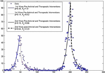
The best-fit trajectory of model (1) along with the daily confirmed cases of H1N1 influenza in Manitoba, Canada. Dashed lines represent post-antiviral and therapeutic interventions for 1st and 2nd wave

Summary

A deterministic model is designed and rigorously analyzed to assess the transmission dynamics and impact of antiviral drugs in curtailing the spread of disease of the 2009 swine influenza pandemic. The analysis of the model, which consists of nine mutually-exclusive epidemiological compartments, shows the following:

• (i)The disease-free equilibrium of the model is shown to be globally-asymptotically stable when ${\displaystyle {\mathcal{R}}_c\le \frac{\mathit{\Omega }}{{\mathit{\theta }}_H}}$.
• (ii)The disease persists in the community if ${\mathcal{R}}_c>1$.
• (iii)The model has a unique endemic equilibrium when the associated reproduction threshold $\left({\displaystyle {\mathcal{R}}_c>\frac{\mathit{\Omega }}{{\mathit{\theta }}_P}}\right)$.
• (iv)Backward bifurcation is observed when all susceptible individuals are equally likely to acquire infection (${\mathit{\theta }}_H=1$) and the vaccination is perfect $({\mathit{\theta }}_P=0)$.
• (v)Uncertainty analysis suggests that with mean value of $R_c=1.32$ and 95 $\%$ confidence interval (1.13, 1.81), the disease will get endemic under the given conditions and data.
• (vi)Sensitivity analysis recommends that we must estimate the parameter values of $\mathit{\beta },{\mathit{\tau }}_1,{\mathit{\varphi }}_T\mathrm{and}{\mathit{\eta }}_4$ with great precision as they greatly influence the magnitude of $R_c,$ which in turn controls the spread of the disease.
• (vii)So far all the analysis is dependent on ${\mathcal{R}}_c$ for the spread of disease. Therefore, we have designed an optimal treatment strategy (using Pontryagin’s maximum principle) to prevent the epidemic. It is observed that the optimal strategy is much more efficient in combating infection with minimal cost and resources.

Appendix

Proof of Lemma 1

Proof

Adding the equations of the model (1) gives

$$\begin{array}{c}\hfill \frac{dN}{dt}=\mathit{\pi }-\mathit{\mu }N-\mathit{\delta }(I_2+{\mathit{\theta }}_{1}H)\le \mathit{\pi }-\mathit{\mu }N.\end{array}$$ 12

Since $N(t)\ge 0$, it follows using a standard comparison theorem [29] that

$$\begin{array}{c}\hfill N(t)\le N(0)e^{-\mathit{\mu }t}+\frac{\mathit{\pi }}{\mathit{\mu }}\left(1-e^{-\mathit{\mu }t}\right).\end{array}$$

Therefore, $N(t)\le \mathit{\pi }/\mathit{\mu }$ if $N(0)\le \mathit{\pi }/\mathit{\mu }$.

This proves the positive invariance of $\mathcal{D}$.

To prove that $\mathcal{D}$ is attracting, from (12), it is clear that $\frac{dN}{dt}<0$, whenever $N(t)>\mathit{\pi }/\mathit{\mu }$. Thus, either the solution enters $\mathcal{D}$ in finite time, or N(t) approaches $\mathit{\pi }/\mathit{\mu }$, and the variables denoting the infected classes approach zero. Hence, $\mathcal{D}$ is attracting and all solutions in ${\mathbb{R}}_{+}^9$ eventually enter $\mathcal{D}$. $\square$

DFE

${\mathcal{R}}_c$ calculation

The matrices F (for the new infection terms) and V (of the transition terms) are given, respectively, by $F=\left[\begin{array}{ccccc}\mathit{\beta }{\mathit{\eta }}_1\mathit{\Omega }& \mathit{\beta }\mathit{\Omega }& \mathit{\beta }{\mathit{\eta }}_2\mathit{\Omega }& \mathit{\beta }{\mathit{\eta }}_3\mathit{\Omega }& \mathit{\beta }{\mathit{\eta }}_4\mathit{\Omega }\\ 0& 0& 0& 0& 0\\ 0& 0& 0& 0& 0\\ 0& 0& 0& 0& 0\\ 0& 0& 0& 0& 0\\ \end{array}\right]$ $V=\left[\begin{array}{ccccc}{K}_1& 0& 0& 0& 0\\ -\mathit{\alpha }f& K_2& 0& 0& 0\\ 0& -\mathit{\gamma }& K_3& 0& 0\\ 0& 0& -\mathit{\psi }& K_4& 0\\ 0& -{\mathit{\tau }}_1& -{\mathit{\tau }}_2& 0& K_5\\ \end{array}\right]$, where, ${\displaystyle \mathit{\Omega }=\frac{S_L^{\ast }+{\mathit{\theta }}_H{S}_H^{\ast }+{\mathit{\theta }}_P{P}^{\ast }}{N^{\ast }},}$ $K_1=\mathit{\alpha }+\mathit{\mu },$ $K_2={\mathit{\tau }}_1+\mathit{\gamma }+\mathit{\mu },$ $K_3={\mathit{\tau }}_2+\mathit{\psi }+{\mathit{\varphi }}_2+\mathit{\mu }+\mathit{\delta },$ $K_4={\mathit{\psi }}_2+{\mathit{\varphi }}_3+\mathit{\mu }+{\mathit{\theta }}_1\mathit{\delta },$ $K_5={\mathit{\varphi }}_T+\mathit{\mu }.$

Reproduction number $R_c$ is given as

$$\begin{array}{c}\hfill R_c=\mathit{\rho }(F{V}^{-1})\end{array}$$

where, $\mathit{\rho }$ denotes the spectral radius.

Proof of Theorem 1

Proof

Consider the model (1) with ${\mathit{\theta }}_H=1$ and ${\mathit{\theta }}_P=0$. Further, consider the Lyapunov function

$$\begin{array}{c}\hfill \mathcal{F}=g_{1}L+g_2{I}_1+g_3{I}_2+g_{4}H+g_{5}T,\end{array}$$

where,

$$\begin{array}{c}\hfill \begin{array}{c}\begin{array}{cc}\hfill g_1& ={\mathit{\eta }}_1{K}_2{K}_3{K}_4{K}_5+\mathit{\alpha }{K}_3{K}_4{K}_5+\mathit{\alpha }{\mathit{\tau }}_1{\mathit{\eta }}_4{K}_3{K}_4+\mathit{\alpha }\mathit{\gamma }{\mathit{\eta }}_2{K}_4{K}_5+\mathit{\alpha }\mathit{\gamma }\mathit{\psi }{\mathit{\eta }}_3{K}_5\hfill \\ \hfill & +\mathit{\alpha }\mathit{\gamma }{\mathit{\tau }}_2{\mathit{\eta }}_4{K}_4\hfill \\ \hfill g_2& =K_1(\mathit{\gamma }{\mathit{\tau }}_2{\mathit{\eta }}_4{K}_5+\mathit{\gamma }\mathit{\psi }{\mathit{\eta }}_3{K}_5+\mathit{\gamma }{\mathit{\eta }}_2{K}_4{K}_5+{\mathit{\tau }}_1{\mathit{\eta }}_4{K}_3{K}_4+K_3{K}_4{K}_5)\hfill \\ \hfill g_3& =K_1{K}_2{K}_5({\mathit{\eta }}_2{K}_4+{\mathit{\eta }}_3+{\mathit{\tau }}_2{\mathit{\eta }}_4)\hfill \\ \hfill g_4& ={\mathit{\eta }}_3{K}_1{K}_2{K}_3{K}_5\hfill \\ \hfill g_5& ={\mathit{\eta }}_4{K}_1{K}_2{K}_3{K}_4\hfill \end{array}\hfill \end{array}\end{array}$$

The Lyapunov derivative is given by (where a dot represents differentiation with respect to t)

$$\begin{array}{cc}\hfill \dot{\mathcal{F}}& =g_1\dot{L}+g_2{\dot{I}}_1+g_3{\dot{I}}_2+g_4{\dot{H}}_1+g_5\dot{T},\hfill \\ \hfill & =g_1[\mathit{\lambda }(S_L+S_H+{\mathit{\theta }}_{P}P)-(\mathit{\alpha }+\mathit{\mu })L]+g_2[\mathit{\alpha }L-({\mathit{\tau }}_1+\mathit{\gamma }+\mathit{\mu })I_1]\hfill \\ \hfill & +g_3[\mathit{\gamma }{I}_1-({\mathit{\tau }}_2+\mathit{\psi }+{\mathit{\varphi }}_2+\mathit{\mu }+\mathit{\delta })I_2]+g_4[\mathit{\psi }{I}_2-({\mathit{\psi }}_2+{\mathit{\varphi }}_3+\mathit{\mu }+{\mathit{\theta }}_1\mathit{\delta })H]\hfill \\ \hfill & +g_5[{\mathit{\tau }}_1{I}_1+{\mathit{\tau }}_2{I}_2-({\mathit{\varphi }}_T+\mathit{\mu })T],\hfill \end{array}$$

so that,

$$\begin{array}{cc}\hfill \dot{\mathcal{F}}& =g_1\mathit{\lambda }[S_L(t)+{\mathit{\theta }}_H{S}_H(t)+{\mathit{\theta }}_{P}P]-K_1{K}_2{K}_3{K}_4{K}_5({\mathit{\eta }}_{1}L+I_1+{\mathit{\eta }}_2{I}_2+{\mathit{\eta }}_{3}H+{\mathit{\eta }}_{4}T),\hfill \\ \hfill & \le g_1\mathit{\lambda }{\mathit{\theta }}_H[S_L(t)+S_H(t)+P(t)]-K_1{K}_2{K}_3{K}_4{K}_5\frac{\mathit{\lambda }N}{\mathit{\beta }},\mathrm{since}{\mathit{\theta }}_P<1<{\mathit{\theta }}_H\hfill \\ \hfill & \le g_1\mathit{\lambda }{\mathit{\theta }}_{H}N-K_1{K}_2{K}_3{K}_4{K}_5\frac{\mathit{\lambda }N}{\mathit{\beta }},\mathrm{since}(S_L(t)+S_H(t)+P(t))\le N(t)\mathrm{in}\mathcal{D}.\hfill \end{array}$$

It can be shown that $g_1=\frac{{\mathcal{R}}_c}{\mathit{\beta }\mathit{\Omega }}{K}_1{K}_2{K}_3{K}_4{K}_5.$ Hence,

$$\begin{array}{cc}\hfill \dot{\mathcal{F}}& \le \frac{{\mathcal{R}}_c}{\mathit{\beta }{R}^{\ast }}{K}_1{K}_2{K}_3{K}_4{K}_5\mathit{\lambda }N-K_1{K}_2{K}_3{K}_4{K}_5\frac{\mathit{\lambda }N}{\mathit{\beta }},\hfill \\ \hfill & =K_1{K}_2{K}_3{K}_4{K}_5\frac{\mathit{\lambda }N}{\mathit{\beta }}(\frac{{\mathcal{R}}_c}{R^{\ast }}-1).\hfill \end{array}$$

Thus, $\dot{\mathcal{F}}\le 0$ if ${\mathcal{R}}_c\le R^{\ast }$ with $\dot{\mathcal{F}}=0$ if and only if $L=I_1=I_2=H=T=0$. Further, the largest compact invariant set in $\{(S_L,S_H,P,L,I_1,I_2,H,T,R)\in \mathcal{D}:\dot{\mathcal{F}}=0\}$ is the singleton $\{{\mathcal{E}}_0\}$. It follows from the LaSalle invariance principle (Chapter 2, Theorem 6.4 of [30]) that every solution to the equations in (1) with ${\mathit{\theta }}_H=1$ and ${\mathit{\theta }}_P=0$ and with initial conditions in $\mathcal{D}$ converges to DFE, ${\mathcal{E}}_0$, as $t\to \infty$. That is, $[L(t),A(t),I_1(t),I_2(t),H(t),H_2(t),T(t)]\to (0,0,0,0,0,0,0)$ as $t\to \infty$. Substituting $L=A=I_1=I_2=H=H_2=T=0$ into the first three equations of the model (1) gives $S_L(t)\to S_L^{\ast },S_H(t)\to S_H^{\ast }$ and $P(t)\to P^{\ast }$ as $t\to \infty$. Thus, $[S_L(t),S_H(t),P(t),L(t),I_1(t),I_2(t),H(t),T(t),R(t)]\to (S_L^{\ast },S_H^{\ast },P^{\ast },0,0,0,0,0,0)$ as $t\to \infty$ for $\widetilde{{\mathcal{R}}_c}\le R^{\ast },$ so that the DFE, ${\mathcal{E}}_0$, is GAS in $\mathcal{D}$ if ${\mathcal{R}}_c\le R^{\ast }$. $\square$

Proof of Theorem 2

Proof

Let X = $\{(S_L,S_H,P,L,I_1,I_2,H,T,R)\in {\mathbb{R}}_{+}^9:L=I_1=I_2=H=T=0\}$. Thus X is the set of all disease free states of (1) and it can be easily verified that X is positively invariant. Let M = $\mathcal{D}\cap X$. Since both $\mathcal{D}$ and X are positively invariant, M is also positively invariant. Also note that ${\mathcal{E}}_0\in M$ and ${\mathcal{E}}_0$ attracts all the solutions in X. So, $\mathit{\Omega }(M)$ = $\{{\mathcal{E}}_0\}$.

By setting $x(t)={(L(t),I_1(t),I_2(t),H(t),T(t))}^T$, equations for the infected components of (1) can be written as

$$\begin{array}{cc}\hfill x^{\prime }(t)& =Y(x)x(t)\hfill \end{array}$$ 13

where Y(x) = $\left[\left(\frac{S_L+{\mathit{\theta }}_H{S}_H+{\mathit{\theta }}_{P}P}{N\mathit{\Omega }}\right)F-V\right]$ and it is clear that $Y({\mathcal{E}}_0)=F-V$. Also it is easy to check that $Y({\mathcal{E}}_0)$ is irreducible. We will apply the Lemma A.4 in [1] to show that M is a uniform weak repeller. Since ${\mathcal{E}}_0$ is a steady state solution, we can consider it to be a periodic orbit of period $T=1$. P(t, x), the fundamental matrix of the solutions for (7) is $e^{tY}$. Since the spectral radius of $Y({\mathcal{E}}_0)={\mathcal{R}}_c-1>0$, the spectral radius of $e^{Y({\mathcal{E}}_0)}>1$. So condition 2 of Lemma A.4 is satisfied. Taking $x={\mathcal{E}}_0$, we get $P(T,{\mathcal{E}}_0)=e^{Y({\mathcal{E}}_0)}$ which is a primitive matrix, because $Y({\mathcal{E}}_0)$ is irreducible, as mentioned in Theorem A.12(i) [40]. This satisfies the condition 1 of Lemma A.4. Thus, M is a uniform weak repeller and disease is weakly persistent. By definition, $M=\mathit{\partial }\mathcal{D}$. M is trivially closed and bounded relative to $\mathcal{D}$ and hence, compact. Therefore by Theorem 1.3 of [42], we have that M is a uniform strong repeller and disease is uniformly persistent. $\square$

Endemic equilibrium

The coefficients are defined as follows

$$\begin{array}{cc}\hfill A_1& =\mathit{\pi }{\mathit{\theta }}_H{\mathit{\theta }}_P\hfill \\ \hfill A_2& =\mathit{\pi }(1-p)[{\mathit{\theta }}_P({\mathit{\sigma }}_H+\mathit{\mu })+{\mathit{\theta }}_H\mathit{\mu }]+\mathit{\pi }{\mathit{\theta }}_{H}p({\mathit{\theta }}_P({\mathit{\sigma }}_L+\mathit{\mu })+\mathit{\mu })+\mathit{\pi }{\mathit{\theta }}_P{A}_1\hfill \\ \hfill A_3& =\mathit{\pi }\mathit{\mu }(1-p)({\mathit{\sigma }}_H+\mathit{\mu })+\mathit{\pi }{\mathit{\theta }}_{H}p\mathit{\mu }({\mathit{\sigma }}_L+\mathit{\mu })+\mathit{\pi }{\mathit{\theta }}_{P}B\hfill \\ \hfill A_4& =\mathit{\pi }(1-p)[{\mathit{\theta }}_P({\mathit{\sigma }}_H+\mathit{\mu })+\mathit{\mu }{\mathit{\theta }}_H]+\mathit{\pi }p[\mathit{\mu }+{\mathit{\theta }}_P({\mathit{\sigma }}_L+\mathit{\mu })]+\mathit{\pi }{A}_1\hfill \\ \hfill A_5& =\mathit{\pi }\mathit{\mu }(1-p)({\mathit{\sigma }}_H+\mathit{\mu })+\mathit{\pi }p\mathit{\mu }({\mathit{\sigma }}_L+\mathit{\mu })+\mathit{\pi }{A}_2\hfill \\ \hfill A_6& =\mathit{\pi }(1-p){\mathit{\theta }}_H{\mathit{\theta }}_P+\mathit{\pi }p{\mathit{\theta }}_P\hfill \\ \hfill A_7& ={\mathit{\sigma }}_L{\mathit{\theta }}_H(1-p)+{\mathit{\sigma }}_{H}p\hfill \\ \hfill A_8& =\frac{1}{K_1}+\frac{\mathit{\alpha }}{K_1{K}_2}+\frac{\mathit{\alpha }\mathit{\gamma }}{K_1{K}_2{K}_3}+\frac{\mathit{\alpha }\mathit{\gamma }\mathit{\psi }}{K_1{K}_2{K}_3{K}_4}+\frac{\mathit{\alpha }{\mathit{\tau }}_1}{K_1{K}_2{K}_5}+\frac{\mathit{\alpha }\mathit{\gamma }{\mathit{\tau }}_2}{K_1{K}_2{K}_3{K}_5}\hfill \\ \hfill & +\frac{\mathit{\alpha }\mathit{\gamma }{\mathit{\varphi }}_{I_2}}{\mathit{\mu }{K}_1{K}_2{K}_3}+\frac{\mathit{\alpha }\mathit{\gamma }\mathit{\psi }{\mathit{\varphi }}_H}{\mathit{\mu }{K}_1{K}_2{K}_3{K}_4}+(\frac{{\mathit{\varphi }}_T}{K_1{K}_5})\frac{\mathit{\alpha }{\mathit{\tau }}_1}{K_1{K}_2{K}_5}+(\frac{{\mathit{\varphi }}_T}{K_1{K}_5})\frac{\mathit{\alpha }\mathit{\gamma }{\mathit{\tau }}_2}{K_1{K}_2{K}_3{K}_5}.\hfill \\ \hfill \end{array}$$

Sensitivity analysis

The estimated parameters are presented in Table 3.

Table 3.

Mean values of the model parameters with their assigned distributions

Parameter	Mean	Distribution	Parameter	Mean	Distribution
$\mathit{\mu }$	3e-5	N	${\mathit{\eta }}_1$	0.1	G
$\mathit{\beta }$	0.5	G	${\mathit{\eta }}_2$	1.2	G
${\mathit{\sigma }}_L$	0.08	N	${\mathit{\eta }}_3$	0.2	G
${\mathit{\sigma }}_H$	0.14	N	${\mathit{\eta }}_4$	0.2	G
$\mathit{\alpha }$	0.35	G	${\mathit{\theta }}_H$	1.2	U
${\mathit{\tau }}_1$	0.5	N	${\mathit{\theta }}_P$	0.3	N
${\mathit{\tau }}_2$	0.6	N	${\mathit{\psi }}_1$	0.5	N
${\mathit{\varphi }}_{I_2}$	0.2	N	${\mathit{\gamma }}_1$	0.06	G
${\mathit{\varphi }}_H$	0.2	N	$\mathit{\delta }$	0.01	N
${\mathit{\varphi }}_T$	0.25	N	${\mathit{\theta }}_1\mathit{\delta }$	0.01	N

N, G and U represents the normal, gamma and uniform distribution respectively

References

- 1.Ackleh, A.S., Maa, B., Salceanua, P.L.: Persistence and global stability in a selection-mutation size-structured model. J. Biol. Dyn. 436–453 (2011)
- 2.Agusto FB. Optimal isolation control strategies and cost-effectiveness analysis of a two-strain avian influenza model. Biol. Syst. 2013;113:155–164. doi: 10.1016/j.biosystems.2013.06.004. [DOI] [PubMed] [Google Scholar]
- 3.Boëlle, P.Y., Bernillon, P., Desenclos, J.C.: A preliminary estimation of the reproduction ratio for new influenza A(H1N1) from the outbreak in Mexico. Euro Surveill. 14 (2000) [DOI] [PubMed]
- 4.Brian, J.C., Bradley, G.W., Sally, B.: Modeling influenza epidemics and pandemics: insights into the future of swine flu (H1N1). BMC Med. 7–30 (2009) [DOI] [PMC free article] [PubMed]
- 5.Canada enters 2nd wave of H1N1. http://www.cbc.ca/health/story/2009/10/23/h1n1-second-wave-canada.html. Accessed 04 Nov 2009
- 6.Centers for Disease Control and Prevention. Three reports of oseltamivir resistant novel influenza A (H1N1) viruses (2009). http://www.cdc.gov/h1n1flu/HAN/070909.htm. Accessed 23 Jan 2010
- 7.Centers for Disease Control and Prevention. http://www.cdc.gov/h1n1flu/background.htm. Accessed 27 Oct 2009
- 8.Centers for Disease Control and Prevention. http://www.cdc.gov/media/pressrel/2009/r090729b.htm. Accessed 27 Oct 2009
- 9.Centers for Disease Control and Prevention (CDC) (2009) Outbreak of swine-origin influenza A (H1N1) virus infection-Mexico. March–April 2009. MMWR Morb. Mortal. Wkly. Rep. 58(Dispatch), 1–3 [PubMed]
- 10.Centers for Disease Control and Prevention. Pregnant women and novel influenza A (H1N1): considerations for clinicians. http://www.cdc.gov/h1n1flu/clinician_pregnant.htm. Accessed 5 Nov 2009
- 11.Centers for Disease Control. Information on people at high risk of developing flu-related complications. http://www.cdc.gov/h1n1flu/highrisk.htm. Accessed 5 Nov 2009
- 12.Cintrón-Arias A, Castillo-Chávez C, Bettencourt LM, Lloyd AL, Banks HT. The esitimation of the effective reproductive number from disease outbreak data. Math. Biosci. Eng. 2009;6(2):261–282. doi: 10.3934/mbe.2009.6.261. [DOI] [PubMed] [Google Scholar]
- 13.Cheng KF, Leung PC. What happened in China during the 1918 influenza pandemic? Int. J. Infect. Dis. 2007;11:360–364. doi: 10.1016/j.ijid.2006.07.009. [DOI] [PubMed] [Google Scholar]
- 14.El Universal, April (2009). http://www.eluniversal.com.mx/hemeroteca/edicion_impresa_20090406.html. Accessed 27 Oct 2009
- 15.Fister, K., Lenhart, S., McNally, J.: Optimizing chemotherapy in an HIV model. Electron. J. Differ. Equ. 1–12 (1998)
- 16.Fleming WH, Rishel RW. Deterministic and Stochastic Optimal Control. Berlin: Springer; 1975. [Google Scholar]
- 17.Fraser, C., et al.: Pandemic Potential of a Strain of Influenza A (H1N1): Early Findings, Science (2009) [DOI] [PMC free article] [PubMed]
- 18.GenBank sequences from 2009 H1N1 influenza outbreak. http://www.ncbi.nlm.nih.gov/genomes/FLU/SwineFlu.html. Accessed 27 Oct 2009
- 19.Gojovic MZ, et al. Modelling mitigation strategies for pandemic (H1N1) Can. Med. Assoc. J. 2009;181:673–680. doi: 10.1503/cmaj.091641. [DOI] [PMC free article] [PubMed] [Google Scholar]
- 20.Hethcote HW. The mathematics of infectious diseases. SIAM Rev. 2000;42:599–653. doi: 10.1137/S0036144500371907. [DOI] [Google Scholar]
- 21.Hiroshi, N., Don, K. et al.: Early epidemiological assessment of the virulence of emerging infectious diseases: a case study of an influenza pandemic, modelling mitigation strategies for pandemic (H1N1). PLoS ONE (2009) [DOI] [PMC free article] [PubMed]
- 22.Influenza Respir. Virus. Virus in North America. 3(2009), 215–222 (2009) [DOI] [PMC free article] [PubMed]
- 23.Jamieson DJ, Honein MA, Rasmussen SA. H1N1 2009 influenza virus infection during pregnancy in the USA. Lancet. 2009;374:451–458. doi: 10.1016/S0140-6736(09)61304-0. [DOI] [PubMed] [Google Scholar]
- 24.Joshi, H.R.: Optimal control of an immunology model. Optim. Control Appl. 199–213 (2002)
- 25.Jung E, Lenhart S, Feng Z. Optimal control of treatments in a two-strain tuberculosis model. Discrete Contin. Dyn. Syst. 2002;B2:473–482. [Google Scholar]
- 26.Kamien ML, Schwartz NL. Dynamic Optimisation. Amesterdam: North Holland; 1991. [Google Scholar]
- 27.Kirschner D, Lenhart S, Serbin S. Optimal control of the chemotherapy of HIV. Math. Biol. 1997;35:775–792. doi: 10.1007/s002850050076. [DOI] [PubMed] [Google Scholar]
- 28.Kumar, A., Zarychanski, R., Pinto, R.: Critically ill patients with 2009 influenza A (H1N1) infection in Canada. J. Am. Med. Assoc. 1872–1879 (2009) [DOI] [PubMed]
- 29.Lakshmikantham V, Leela S, Martynyuk AA. Stability Analysis of Nonlinear Systems. New York: Marcel Dekker Inc; 1989. [Google Scholar]
- 30.LaSalle JP. The Stability of Dynamical Systems. Regional Conference Series in Applied Mathematics. Philadelphia: SIAM; 1976. [Google Scholar]
- 31.Manitoba Health: Confirmed Cases of H1N1 Flu in Manitoba. http://www.gov.mb.ca/health/publichealth/sri/stats1.html. Accessed 31 Dec 2009
- 32.Nuno M, Chowell G, Gumel AB. Assessing transmission control measures, antivirals and vaccine in curtailing pandemic influenza: scenarios for the US, UK, and The Netherlands. Proc. R. Soc. Interf. 2007;4:505–521. doi: 10.1098/rsif.2006.0186. [DOI] [PMC free article] [PubMed] [Google Scholar]
- 33.Olson DR, Simonsen L, Edelson PJ, Morse SS. Epidemiological evidence of an early wave of the 1918 influenza pandemic in New York City. Proc. Natl. Acad. Sci. USA. 2005;102:11059–11063. doi: 10.1073/pnas.0408290102. [DOI] [PMC free article] [PubMed] [Google Scholar]
- 34.Peter, C., Franco-Paredes, C., Preciado, J.I.S.: The first influenza pandemic in the new millennium: lessons learned hitherto for current control efforts and overall pandemic preparedness. J. Immune Based Therap. Vacc. (2009) [DOI] [PMC free article] [PubMed]
- 35.Pontryagin LS, Boltyanskii VG. The Mathematical Theory of Optimal Processes. New York: Golden and Breach Science Publishers; 1986. [Google Scholar]
- 36.Public Health Agency of Canada. http://www.phac-aspc.gc.ca/fluwatch/09-10/w45_09/index-eng.php. Accessed 9 March 2010
- 37.Public Health Agency of Canada. http://www.phac-aspc.gc.ca/fluwatch/09-10/w07_10/index-eng.php. Accessed March 2010
- 38.Samsuzzoha Md, Singh M, Lucy D. Numerical study of a diffusive epidemic model of influenza with variable transmission coefficient. Appl. Math. Model. 2007;35:5507–5523. doi: 10.1016/j.apm.2011.04.029. [DOI] [Google Scholar]
- 39.Swine influenza (H1N1) pandemic. Bull. Math. Biol. 73(2011), 515–548 (2009) [DOI] [PubMed]
- 40.Smith HL, Waltman P. The Theory of the Chemostat. Cambridge: Cambridge Univ. Press; 1995. [Google Scholar]
- 41.Taubenberger JK, Reid AH, Fanning TG. The 1918 influenza virus: a killer comes into view. Virology. 2000;274:241–245. doi: 10.1006/viro.2000.0495. [DOI] [PubMed] [Google Scholar]
- 42.Thieme, H.R.: Persistence under relaxed point-dissipativity. SIAM J. Math. Anal. 407–435 (1993)
- 43.Tharakaraman K, Sasisekharan R. Cell Host Microb. 2015;17:279–282. doi: 10.1016/j.chom.2015.02.019. [DOI] [PubMed] [Google Scholar]
- 44.van den Driessche P, Watmough J. Reproduction numbers and sub-threshold endemic equilibria for compartmental models of disease transmission. Math. Biosci. 2002;180:29–48. doi: 10.1016/S0025-5564(02)00108-6. [DOI] [PubMed] [Google Scholar]
- 45.Winnipeg Regional Health Authority Report. Outbreak of novel H1N1 influenza A virus in the Winnipeg health region. http://www.wrha.mb.ca/. Accessed 4 Nov 2009
- 46.World Health Organization, Influenza: Data and Statistics. http://www.euro.who.int/en/health-topics/communicable-diseases/influenza/data-and-statistics
- 47.World Health Organization. Pandemic (H1N1) (2009)-update 71. http://www.who.int/csr/don/2009_10_23/en/index.html. Accessed 27 Oct 2009
- 48.World Health Organization. Influenza A (H1N1)-update 49. Global Alert and Response (GAR). http://www.who.int/csr/don/2009_06_15/en/index.html. Accessed 27 Oct 2009
- 49.World Health Organization. Statement by Director-General. June 11, 2009
- 50.World Health Organization. Human infection with new influenza A (H1N1) virus: clinical observations from Mexico and other affected countries. Weekly epidemiological record, May 2009; 84:185. http://www.who.int/wer/2009/wer8421.pdf. Accessed 5 Nov 2009
- 51.World Health Organization. Pandemic (H1N1) 2009—update 81. http://www.who.int/csr/don/2010_03_05/en/index.html. Accessed 5 March 2010
- 52.Yan X, Zou Y, Li J. Optimal quarantine and isolation strategies in epidemics control. World J. Mod. Simul. 2007;33:202–211. [Google Scholar]