Foundations of modeling in cryobiology---II: Heat and mass transport in bulk and at cell membrane and ice-liquid interfaces

Abstract

Modeling coupled heat and mass transport in biological systems is critical to the understanding of cryobiology. In Part I of this series we derived the transport equation and presented a general thermodynamic derivation of the critical components needed to use the transport equation in cryobiology. Here we refine to more cryobiologically relevant instances of a double free-boundary problem with multiple species. In particular, we present the derivation of appropriate mass and heat transport constitutive equations for a system consisting of a cell or tissue with a free external boundary, surrounded by liquid media with an encroaching free solidification front. This model consists of two parts–namely, transport in the “bulk phases” away from boundaries, and interfacial transport. Here we derive the bulk and interfacial mass, energy, and momentum balance equations and present a simplification of transport within membranes to jump conditions across them. We establish the governing equations for this cell/liquid/solid system whose solution in the case of a ternary mixture is explored in Part III of this series.

1. Introduction

Continuum descriptions of transport processes in and between fluid, solid and vapor phases play a central role in the current understanding of physical, chemical and biological systems. Transport equations for mass, momentum, energy and species are ubiquitous in the corresponding model formulations. Indeed well-known textbooks on continuum mechanics (e.g. Malvern [108]), transport processes (e.g. Bird, Stewart and Lightfoot [29]), fluid mechanics (e.g. Lamb [93], Batchelor [21], Landau and Lifshitz [95]), elasticity and solid mechanics (e.g. Chau and Pagano [43], Landau and Lifshitz [94]), biomechanics (e.g. Fung [54–56]) and heat transfer (e.g. Carslaw and Jaeger [39]) are indispensable resources for anyone working in these fields. Sitting at the intersection of these fields is cryobiology.

The systems that these continuum models describe generally involve not only transport in individual bulk phases (fluid, solid or vapor) but also transport processes that occur at and/or across the interface between phases. Transport processes associated with an interface naturally arise in the study of phase transformation processes such as solidification [46, 59] and evaporation/condensation [37] and can be the dominant effects in situations such as thin film flows [126]. An important distinction for a domain boundary is whether it is a material boundary across which no mass is transferred (e.g. an impermeable container wall or a boundary between two immiscible liquids), a boundary at which phase transformation occurs (e.g. a freezing/melting solid–liquid interface or an evaporating/condensing liquid–vapor interface), or neither of the above such as a semi-permeable membrane [166] across which mass is transferred but no change of phase takes place. Characterizations of fluid–fluid interfacial phenomena include those that arrive at mathematical conditions applied at a ‘sharp’ interface through the recognition that in reality there exists a transition region of nonzero thickness separating the two phases (e.g. see [112, 113]). Computational approaches that treat the interface as having a nonzero thickness such as diffuse-interface methods for fluid–fluid systems [9] and phase-field methods applied to solidification and materials science phenomena [34, 153] are well-suited for systems with complex interface morphology (e.g. dendritic crystal growth) and/or changes in topology. The level set method [147, 148] is another computational approach that defines the interface between two phases implicitly to allow for efficient tracking of complex interface shapes and topologies. Level set methods have been used extensively in systems undergoing phase transformation and have seen recent application in the cryobiology literature [40, 106].

Continuum theories have also been developed to describe multi-phase systems in which two or more phases exist in close proximity such as porous materials [23] and other ‘mixtures’ of fluids, solids and/or gases. In particular, transport models in these systems have been developed using continuum of mixtures approaches [18, 35] as well as averaging procedures and hybrid mixture theory [26, 27, 61, 67–69]. Applications of these and related models cover a wide range that includes, for example, geophysics of soils [28, 124], industrial materials processing and filtration systems [5, 131], paper and inkjet printing industries [7, 51], pharmaceutical science and drug delivery [161] and soft-tissue biomechanics [1, 17, 19, 20, 70, 79, 92, 122].

Phase transformation—and in particular, solidification—of multi-component solutions is a central aspect of cryobiology and cryopreservation that has also been developed deeply in other fields. These related areas include industrial processing of metal alloys and materials growth applications [25, 53, 87–89, 145], geophysical systems such as sea ice [125, 136, 137, 157, 165] and magma chambers [71], as well as laboratory systems with ternary salt solutions that include effects of convection and growth of mushy zones [4, 6, 8, 10, 31, 65, 155, 171, 172]. Inward solidification of an enclosed fluid volume has been the subject of analytical and numerical investigations for specialized geometries such as slabs, circular cylinders and spheres for pure materials [117, 118, 127, 135, 140] and binary melts [50]. Solidification in other simple geometries has been examined to explore effects of thermal stresses and elastic/plastic solid deformation [134] and also phase-change expansion, the pressure-dependence of the melting temperature and the elastic response of the container [44]. Solidification towards and possible engulfment or ‘pushing’ of bubbles, particles and biological cells as well as other particle–solidification front interactions is also a well-studied problem (e.g. [38, 40, 58, 75, 85, 138, 139, 164]) that has implications for cryopreservation. The related problem of solidification of colloidal suspensions has also been examined [128, 129].

In cryobiology, bulk transport processes (in solid, liquid and/or intracellular regions) occur alongside interfacial processes associated with solidification and are coupled to transport processes across a semipermeable cell membrane. Cryobiology as such lies at the nexus of thermal and chemical transport, fluid and solid mechanics, biomechanics, and solidification. The importance of interactions between the physical chemistry of solutions and the physiology of membrane transport has long been recognized as crucial for successful cryopreservation (e.g. [114, 115]). These bio-thermo-chemical interactions are at play in the “two-factor hypothesis” [115], which suggests that optimal cooling rates for cryopreservation lies somewhere between ‘too fast’ – where the cell does not dehydrate sufficiently to avoid intracellular ice formation – and ‘too slow’ – where the cell is overexposed to high solute concentrations. The two-factor hypothesis has been broadly applicable (although given the diversity of cryopreservation specimens understandably not universally applicable) and has guided researchers seeking optimal cooling and warming strategies in various settings. A more detailed discussion of these developments can be found in the introductory section of Part I of this series [11] and references therein.

The identification of optimal cryo-protocols for cooling and warming is further linked to chemical processes in that successful cryopreservation typically involves the introduction of cryoprotective agents, or CPAs. These chemicals (e.g. glycerol, ethylene glycol, propylene glycol) are membrane permeable and their introduction is intended to (1) safely reduce the relative intracellular salt concentration by replacing, through membrane transport processes, intracellular water with CPAs and (2) reduce intracellular ice formation by promoting glass formation (vitrification). The presence of multiple chemical species require that cell membrane transport models account for both water transport and CPA transport. The ‘Two-Parameter’ [72, 78] and ‘Kedem-Katchalsky’ [80, 81] models are two that are commonly used in cryobiology. These and related ones have been reviewed by Kleinhans [83] and Elmoazzen et al. [49].

Other issues connected to questions of transport that are of particular importance in cryobiology include modeling of viscosity and intracellular glass formation [16, 60, 121], prediction of intracellular ice formation and ice nucleation [76, 123], ice front stability [109], mushy layer formation [158], treatment of non-ideal and non-dilute transport models and phase diagrams [47, 49, 84, 100, 132, 162, 163], identification of material properties and their temperature dependence in subzero, cryogenic regimes [42], differentiation between osmotically active and inactive regions within the cell [22] and solid/soft-tissue mechanics of the cell and membrane [32, 33, 73, 74, 116]. Cryopreservation of tissues, compared to that of a single cell, gives rise to additional issues related to their larger size and complex shapes as well as issues related to the presence of vascular structures [30, 142], layered tissues (e.g. epidermis, dermis) [167, 173] and reduced mass transfer rates such as in articular cartilage [96]. A detailed review addressing challenges in the cryopreservation of tissues can be found in Karlsson and Toner [77]. A recent review of physical, mechanical, and chemical processes of importance in cryobiology can be found in Zhmakin [175]. Additionally, an excellent introductory biophysical survey of the field of cryobiology can be found in the book by Zhmakin [176].

In Part I of the series [11], where further discussion of many of the issues raised in the preceding paragraph also can be found, we argued that understanding coupled heat and mass transport in cells and tissues is critical for low temperature biology and for optimizing cryoprotocols. There we identified a general transport equation, expressed in terms of a total flux (e.g. involving convective and/or diffusive fluxes) for a conserved quantity (e.g. mass or energy) and reviewed standard choices for the representation of chemical compositions in a solution. The constitutive laws that typically are used to describe the flux of a particular chemical species, for example, are written in terms of the gradient of the chemical potential. Motivated by this, the remainder of Part I focused on the derivation of chemical potential gradients in various formats of relevance in cryobiology (in terms of mole fraction in the main document [11] and molality and concentration in the supplement [12]).

In the present manuscript we describe our choices for constitutive laws governing the fluxes and then derive the resulting transport equations in two spatial settings—in the “bulk” and at an interface (see Figure 1). First, we present the general heat and mass transport models away from interfaces (i.e. bulk transport). Second, we account for transport at interfaces independently via balance equations for chemical species and energy. This interfacial transport is locally dependent on mass, momentum, molar, and energy balances that depend on a wide variety of effects and is one of the key challenges in modeling these systems. Additional complicating interfacial effects arise from phase-change and solubility considerations. In this manuscript we describe approaches to each of these phenomena, focusing on the model derivation for multicomponent systems. Further, in part III of this series [13] we explore solutions of the model proposed here for the case of ternary mixtures and connect the results to those of related models.

Figure 1:

Regions under consideration. Solid lines indicate interfaces. Bulk transport occurs away from solid lines. Here we make no assumptions about region geometry.

The formulation given below incorporates multiple cryobiological processes acting over a wide range of length and time scales. Nonetheless, our model is not meant to be exhaustive of all possible physical, chemical and biological processes of importance in cryobiology. For example, we have not included a treatment of ionic transport, though neglecting ionic transport is a standard cryobiological assumption. Including this feature here would add considerable complexity to the present model due to requiring a spatially dependent electric potential model, a model of membrane potential, a model of active ionic transport, etc. This assumption can be justified in the classical sense because the contribution of ionic transport to intracellular freezing point depression, and thus the likelihood of intracellular ice, is minimal compared to the contributions of cryoprotective agents. However this is an area of our present research. Additionally, while we do include fluid mechanical processes to some degree, we have omitted from the actual models other mechanical considerations of the cell and cell membrane such as elasticity and/or membrane bending forces. It is our hope that the model established in the present work can be used as a framework upon which other such processes may be explored further.

The rest of the paper is organized as follows. In Section 2 we derive equations for bulk transport away from boundaries. In Section 3 we discuss interfacial conditions including various balance equations and also interfacial conditions specific for a solidification front. In Section 4 we discuss transport in a semipermeable cell membrane. In Section 5 we adapt the membrane transport to jump conditions across the membrane. We close with a discussion and conclusions in Section 6.

2. Transport in Bulk Phases Away From Boundaries

In this section we outline equations for chemical and thermal transport applicable for the solid, liquid and intracellular regions away from their interfaces. We treat interfacial conditions and their effects on the models in Section 3.

2.1. Species Diffusion Equations

Briefly, in part I of this series we used a conservation principle to derive a balance equation that incorporated a composition variable (e.g. density) and a flux (see Part I, equation (27)). This is a continuum-type description of the transport that identifies with each point in the macroscale domain an infinitesimal volume element that, if viewed on the molecular scale, encompasses a large number of molecules. The number of molecules of a particular species occupying that volume allows for the definition of a concentration c_i of species i at that point in space and time. Other bulk quantities such as density and temperature can similarly be assigned in the continuum description. For a multicomponent fluid system such as the one under consideration here, one can identify at each point in space and time a fluid velocity for the mixture as a whole and also velocities representative of each chemical species. This gives rise to a choice of a point or “frame” of reference. When a pure fluid is flowing through a pipe or some other fixed apparatus in the lab, it is natural to define its (bulk) velocity relative to stationary pipe walls (e.g. the lab frame). For a fluid mixture of chemical species, in order to distinguish diffusive motion (e.g. that driven by gradients of chemical potentials) from convective motion (e.g. that driven by a bulk stirring motion that would transport passive particles as well as reactive chemicals) it is necessary to first identify at each point in space and time a velocity, v_i, associated with each species i as well as a velocity v that is representative of the fluid motion as a whole. Here v_i can be defined in a similar manner to the other continuum variables described above and may, for example, be specified with respect to a fixed (lab) frame of reference. Owing to the various convective and diffusive processes present in a multicomponent system the velocity of one species at a given point in space and time may differ from the velocity of another species at the same point in space and time and these velocities may differ from the velocity v associated with the infinitesimal volume element as a whole. Here it is this relative motion that we must address. An appropriate stage for this discussion is the balance equation for the concentration c_i of species i (as derived in Part I), given by¹

$$\frac{\partial c_i}{\partial t}+\nabla \cdot J_i^0=0,$$ (1)

where the molar flux of species i measured in the laboratory frame (i.e. with respect to a fixed position):

$$J_i^0=c_i{v}_i.$$ (2)

These and other variables that appear are defined in Table 1.

Table 1:

Parameter definitions, subscript i indicates quantities associated with species i

Parameter	Name
c	Concentration
t	Time
∇	Gradient operator
J0	Molar flux in the laboratory frame
v	Local mass averaged velocity
N	Moles
M	Molar mass
ω	Mass fraction
ρ	Density
JB	Molecular mass flux
μ	Chemical potential
${\mathcal{M}}^B$	Solute mobility coefficient
${\overline{S}}^c$	Partial molar entropy
${\overline{V}}^c$	Partial molar volume
$D_{ij}^c$	Diffusion coefficient for species i that depends on the gradient of concentration j for concentration derived chemical potential
P	Pressure
GM/Gmolal	Gibbs energy in molar or molal form
DB	Diffusivity
h	Enthalpy
Q	Total heat flux
T	Temperature
cp	Specific heat
k	Thermal conductivity
κ	Thermal diffusivity
F	Fluid body force
σ	Fluid stress tensor
μv	Dynamic viscosity
VI	Interfacial velocity
Vn	Normal velocity
$\widehat{n}$	Normal direction
A	Area
+/−	Superscripts indicate quantities on opposite sides of an interface
Jmass	Mass flux
Jvol	Volume flux
L	Latent heat of solidification (fusion) per unit mass
α/β	Superscripts indicate quantities associated with different phases
K0	Solid/liquid solute partition coefficient
μK	interface mobility parameter
$\mathcal{K}$	Twice mean interfacial curvature

We take the bulk fluid velocity at each point in space and time to be defined as the mass averaged velocity

$$v=\frac{{\sum }_{i=1}^n{N}_i{M}_i{v}_i}{{\sum }_{i=1}^n{N}_i{M}_i}=\sum _{i=1}^n{\omega }_i{v}_i,$$ (3)

which uses the barycentric (mass averaged) velocity frame (e.g. see Bird et al. [29]). Here N_i is the number of moles of species i, M_i is the molecular mass of species i and ω_i is the mass fraction of species i (see also Anderson et al. [11]). Then the molecular mass flux of i (the flow of mass of the i-component through a unit area per unit time relative to the barycentric velocity) is defined to be

$$J_i^{\text{B}}={\rho }_i\left(v_i-v\right),$$ (4)

where ρ_i is the mass concentration of species i. As such, $J_i^{\text{B}}$ measures the extra motion of species i over and above the bulk convective motion of the fluid. As noted by Dantzig et al. [45], with v_i and v both given with respect to the lab frame, the quantity $J_i^{\text{B}}$ is frame independent. It is the quantity $J_i^{\text{B}}$ that in the next section we shall identify as driven by a chemical potential gradient. Using ρ_i = M_ic_i, we have

$$J_i^0=\frac{1}{M_i}{J}_i^{\text{B}}+c_{i}v.$$ (5)

This leads to the species balance equations

$$\frac{\partial c_i}{\partial t}+\nabla \cdot \left(c_{i}v\right)+\frac{1}{M_i}\nabla \cdot J_i^{\text{B}}=0,$$ (6)

for i = 1,2,…,n. In terms of the mass concentration ρ_i we have

$$\frac{\partial {\rho }_i}{\partial t}+\nabla \cdot \left({\rho }_{i}v\right)+\nabla \cdot J_i^{\text{B}}=0.$$ (7)

See also equation (19.1–7) in Bird, Stewart & Lightfoot [29] (p. 583). Other possible frames of reference include the ‘volume averaged velocity frame’ examined by Dantzig et al. or the ‘molar average velocity frame’ described in Bird et al. [29]. For more detailed discussions of diffusion fluxes, reference frames and different velocity fields see Bird, Stewart and Lightfoot [29], Dantzig et al. [45], Sekerka [146] and also Andersson and Ågren [15].

Note that the sum over all molecular mass fluxes is zero:

$$\sum _{i=1}^n{J}_i^{\text{B}}=\sum _{i=1}^n{\rho }_i{v}_i-\sum _{i=1}^n{\rho }_{i}v=\rho \sum _{i=1}^n{\omega }_i{v}_i-v\sum _{i=1}^n{\rho }_i=\rho v-v\rho =0,$$ (8)

where ρ is the mass density of the solution. Therefore, summing equations (7) over i = 1,…,n, and using $\sum {\rho }_i=\rho$, we have

$$\frac{\partial \rho }{\partial t}+\nabla \cdot \left(\rho \mathit{v}\right)=0.$$ (9)

This is the standard mass conservation equation of continuum fluid dynamics. These results can also be expressed in terms of other concentration variables through the relationships outlined in Section 2 of Part I of this series [11].

2.1.1. Constitutive Equation for Diffusive Flux $J_i^{\text{B}}$

In Part I of the series, we derived the fundamental conservation law (Eq. (27) in [11]) and suggested that the diffusion flux it contains is supplanted with a constitutive model. In particular, a standard constitutive model (see, e.g. [29]) for the diffusive flux $J_i^{\text{B}}$ assumes the flux is proportional—via a mobility coefficient ${\mathcal{M}}_i^{\text{B}}$ that may depend on concentration, temperature, etc.—to the concentration times the chemical potential gradient:

$$J_i^{\text{B}}=-{\mathcal{M}}_i^{\text{B}}{c}_i\nabla {\mu }_i,\text{\hspace{1em}\hspace{1em}for}i=1,\dots ,n,$$ (10)

where it then remains to identify appropriate forms for the chemical potentials μ_i for each species i. We accomplish this by first identifying a general form for the Gibbs Free Energy and then obtaining the associated chemical potential gradients. These details, in terms of mole fraction x_i, molality m_i and concentration c_i, are given in Part I of this series [11] and its associated supplement [12]. Into these results one can then insert a specific choice for the Gibbs Free Energy, such as that proposed for cryobiological applications with ternary systems by Elliott et al. [47, 49].

For the ternary case the chemical potential gradients can be expressed in terms of temperature, pressure and concentration gradients (see Part I Supplement [12] equation (34)). In this case, the fluxes are

$$J_i^{\text{B}}=-{\mathcal{M}}_i^{\text{B}}{c}_i\left(-{\overline{S}}_i^{\text{c}}\nabla T+{\overline{V}}_i^{\text{c}}\nabla P+D_{i2}^{\text{c}}\nabla c_2+D_{i3}^{\text{c}}\nabla c_3\right),\text{\hspace{1em}\hspace{1em}for}i=1,2,3,$$ (11)

where the multipliers of the gradient terms, ${\overline{S}}_i^c$ (partial molar entropy), ${\overline{V}}_i^{\text{c}}$ (partial molar volume) and $D_{ij}^{\text{c}}$ (diffusion coefficient) are defined in terms of either G_M or G_molal in equations (35)–(37) in Part I Supplement [12].

Inserting these expressions for $J_i^{\text{B}}$ into Eq. (6) for i,j = 2,3, i ≠ j gives

$$\frac{\partial c_i}{\partial t}+\nabla \cdot \left(c_{i}v\right)=\frac{1}{M_i}\nabla \cdot \left[{\mathcal{M}}_i^{\text{B}}{c}_i\left(-{\overline{S}}_i^{\text{c}}\nabla T+{\overline{V}}_i^{\text{c}}\nabla P+D_{ii}^{\text{c}}\nabla c_i+D_{ij}^{\text{c}}\nabla c_j\right)\right].$$ (12)

If desired, an equation for c₁ can also be written down. In the event that the influence of temperature gradients, pressure gradients and cross diffusion gradients (i.e. the ∇c_j term in the c_i equation) can be neglected these equations reduce to well-known and standard advection-diffusion equations

$$\frac{\partial c_i}{\partial t}+\nabla \cdot \left(c_{i}v\right)=\nabla \cdot \left(D_i^{\text{B}}\nabla c_i\right),i=2,3,$$ (13)

where the diffusivities are $D_i^{\text{B}}:={\mathcal{M}}_i^{\text{B}}{c}_i{D}_{ii}^{\text{c}}/M_i$, i = 2, 3.

It is worth keeping in mind our intended modeling context where we shall assume for simplicity that the quantity

$$\nabla \cdot \left[{\mathcal{M}}_i^{\text{B}}{c}_i\left(-{\overline{S}}_i^{\text{c}}\nabla T+{\overline{V}}_i^{\text{c}}\nabla P+D_{ij}^{\text{c}}\nabla c_j\right)\right],i\ne j,$$ (14)

can be neglected. In general, however, the ramifications of assuming that these effects are negligible must be carefully evaluated in cryobiological settings especially when quantitative predictions are desired. We will see that often this assumption is reasonable due to time-scale issues: while there are temperature gradients, for example, the time-scale on which they are relatively large is much shorter than that of concentration. We discuss this assumption under more specific conditions in Part III of this series [13].

2.2. Thermal Diffusion Equation

For a system undergoing thermal change, the heat energy balance equation (e.g. see equation (27) in Part I of the series) can be written

$$\frac{\partial \left(\rho h\right)}{\partial t}+\nabla \cdot Q=0,$$ (15)

where h is the enthalpy per unit mass and Q is the total heat flux. Using the usual constitutive equation for total heat flux, we assume that Q has a Fourier conduction term and a convective term given by

$$Q=-k\nabla T+\rho hv,$$ (16)

where k is the thermal conductivity of the material, and v is the barycentric fluid velocity. It follows that

$$h\left[\frac{\partial \rho }{\partial t}+\nabla \cdot (\rho v)\right]+\rho \left(\frac{\partial h}{\partial t}+v\cdot \nabla h\right)=\nabla \cdot (k\nabla T).$$ (17)

Upon using equation (9) and assuming h = h(T) with specific heat of the material defined by ∂h/∂T = c_p we obtain the diffusion equation for temperature

$$\rho c_p\left(\frac{\partial T}{\partial t}+v\cdot \nabla T\right)=\nabla \cdot (k\nabla T).$$ (18)

2.3. Linear Momentum Equation

The fluid velocity v in the liquid region satisfies the momentum balance

$$\rho \left(\frac{\partial v}{\partial t}+v\cdot \nabla v\right)=\nabla \cdot \sigma +F\text{,}$$ (19)

where σ is a stress tensor appropriate for the fluid, F is a body force, and ∇·σ acts on each row of σ independently. For example, for a Newtonian fluid

$$\sigma =-PI+{\mu }_{\text{v}}\left(\nabla v+\nabla v^T\right)-\frac{2}{3}{\mu }_{\text{v}}(\nabla \cdot v)I,$$ (20)

where I is the identity matrix, P is the pressure and μ_v is the dynamic viscosity (e.g. see Batchelor [21]).

Our primary focus in the present work will be on diffusive processes and so we limit our discussion of hydrodynamic processes here. We note, however, that the role of hydrodynamics has been recently investigated in dynamics of semipermeable biological membranes near substrates [32] and vesicles in the presence of electric fields [116].

3. Interfacial Conditions

The problem under consideration involves an interface that separates solid and liquid phases as well as a cell membrane that separates the intra- and extracellular regions. In fact, the cell membrane is a distinct, albeit thin, region in its own right bounded by a cell–membrane interface on the inside and a membrane– liquid interface on the outside. For the solid–liquid interface, we develop the basics here but the reader may also refer to books on solidification by Kurz and Fisher [90] and by Davis [46]. There is considerable effort to understand specific pathways of transport through membranes, whether through channels, pores, bilayer diffusion, etc (c.f. [52, 91]). These models, however, while detailed and accurate in some sense as they account for very specific structures, rely on phenomenological or experimental validation when applied to whole cells in different environments in the same way as a lumped “membrane permeability” model: different modes of transport for different species will have different relative contributions, which may be differentially affected by concentrations of other solutes, nonidealities, etc. These complications must be well characterized in the contexts that the model will be used. Because of the highly nonideal nature of modeling during cryopreservation and the multiple solutes and paths by which species cross the membrane, it is considerably simpler and likely as accurate in our application to use a phenomenological, lumped parameter model. Therefore, our objective in Section 4 is to develop a model that can treat the membrane as a mathematical boundary of zero thickness.

To begin our discussion of interfacial conditions we outline general balances separating two phases with special attention paid to the case of a solid–liquid interface. Additional interfacial conditions specific to a solidifying interface are given in Section 3.5. Then the identification of appropriate jump conditions involving intracellular and extracellular variables is made by first examining models for transport processes within the membrane (Section 4) and then applying this information to interfacial conditions at the cell–membrane and membrane– liquid interfaces (Section 5).

In the following sections, we consider an arbitrary region of interface with cross sectional area A separating two phases (denoted as a ‘−’ phase and a ‘+’ phase) with unit normal $\widehat{n}$ pointing into the ‘+’ phase (see Fig. 2). In the laboratory frame the velocity of the interface is denoted by V_I and the normal velocity of the interface is $V_{\text{n}}=V_{\text{I}}\cdot \widehat{n}$. Quantities on either side of the interface are indicated with ‘+’ or ‘−’ superscripts. Conservation laws applied over an infinitesimal time interval dt can then be stated. The conditions derived will be general in the sense that they include the effects of diffusion, convection and phase transformation although some of these effects will later be excluded in our reduced models.

Figure 2:

Schematic of a typical pillbox balance equation. We assume the total width dx⁺ + dx⁻ and cross sectional area A are constant from time t to t + dt. We have that $d{x}^{-}=d{x}_{\text{o}}^{-}+V_{\text{n}}$ and $d{x}^{+}=d{x}_{\text{o}}^{+}-V_{\text{n}}dt$. The volume in the left region at time t, for example, is given by $Ad{x}_{\text{o}}^{-}$, and if, for example, [ρ] =mass/volume, then the mass at time t is ${\rho }^{-}Ad{x}_{\text{o}}^{-}+{\rho }^{+}Ad{x}_{\text{o}}^{+}=\left({\rho }^{-}d{x}_{\text{o}}^{-}+{\rho }^{+}d{x}_{\text{o}}^{+}\right)A$ and the mass at time t + dt is $\left({\rho }^{-}d{x}^{-}+{\rho }^{+}d{x}^{+}\right)A={\rho }^{-}\left(d{x}_{\text{o}}^{-}+V_{\text{n}}dt\right)A+{\rho }^{+}\left(d{x}_{\text{o}}^{+}-V_{\text{n}}dt\right)A$. The change of mass from t to t + dt is then (ρ⁻ − ρ⁺)V_nAdt. On the other hand, note that if the velocity into the left region is v⁻ and the velocity out of the right region is v⁺, then the normal velocity is $v\cdot \widehat{n}$ and the mass flux over time dt is $\left({\rho }^{-}{v}^{-}-{\rho }^{+}{v}^{+}\right)\cdot \widehat{n}Adt$.

3.1. Interfacial Mass Balance

Given mass density ρ, conservation of mass at an interface region of cross sectional area A over an infinitesimal interval in time dt can be stated as

$$\left({\rho }^{-}-{\rho }^{+}\right)V_{\text{n}}Adt=\left({\rho }^{-}{v}^{-}-{\rho }^{+}{v}^{+}\right)\cdot \widehat{n}Adt,$$ (21)

at the interface (see Fig. 2). The left hand side of this equation represents the change in mass associated with an infinitesimal motion of the interface and is nonzero at a moving interface if the densities of the two phases are different.

Suppose, for example, the ‘−’ region is ice and the ‘+’ region is water. Then, ρ⁺ > ρ⁻, and if V_n > 0, the left hand side of Eq. (21) can be interpreted as a decrease in mass in an infinitesimally thin ‘pillbox’ volume encompassing the representative interfacial area; i.e. the more dense water is ‘pushed’ out of the ‘+’ phase side of the pillbox and is replaced by the same volume of less dense ice entering the ‘−’ phase side. The right hand side of Eq. (21) represents the net mass transport carried across a region of area A in the ‘+’ and ‘−’ phases and must match the net mass change represented by the left-hand-side term.

Equation (21) can be rewritten as

$${\rho }^{+}\left(v^{+}-V_{\text{I}}\right)\cdot \widehat{n}={\rho }^{-}\left(v^{-}-V_{\text{I}}\right)\cdot \widehat{n},$$ (22)

where ρ⁺ and ρ⁻ denote bulk densities and v⁺ and v⁻ denote velocities (all evaluated at the interface). In this form, this is a statement that the mass flux $J_{\text{mass}}:=\rho \left(v-V_{\text{I}}\right)\cdot \widehat{n}$ (c.f. Eq. (4)) is continuous across the interface. This condition must hold regardless of whether or not the mass flux across the interface is zero (i.e. a material or phase boundary). For example, at a material boundary where J_mass = 0 we have the conditions that $v^{+}\cdot \widehat{n}=v^{-}\cdot \widehat{n}=V_{\text{I}}\cdot \widehat{n}$, while at a boundary undergoing phase transformation a nonzero J_mass may be related to quantities such as temperature or solute gradients. Note that if the densities are the same on both sides of the boundary, ρ⁺ = ρ⁻, then (22) reduces to $v^{+}\cdot \widehat{n}=v^{-}\cdot \widehat{n}$. In such a context it is useful to define the volume flux across the interface as $J_{\text{vol}}:=\left(v-V_{\text{I}}\right)\cdot \widehat{n}$, which would be equal on both sides.

3.2. Interfacial Momentum Balance

Stress balances for normal and tangential components of σ · nˆ would apply at a fluid–fluid interface (see, for example, Batchelor [21]) but the present situation has fluid–solid and fluid–cell membrane boundaries. At the solidification front a no-slip condition is standard along with conditions on the normal velocity discussed above. A stress balance at the fluid–cell membrane boundary in general must account for not only viscous stresses in the fluid regions but also the bending stiffness and incompressibility of the membrane [32] as well as external stresses such as those associated with the presence of electric fields [116]. For instances with vesicles attached to or near a substrate additional attractive and repulsive forces between the membrane and the substrate must be considered [32, 33]. While a thorough description of membrane deformation must account for these types of stresses, for simplicity our present focus will be on thermal and multi-species diffusive transport across the membrane rather than the membrane mechanics.

3.3. Interfacial Solute Balance

For balances of specific chemical species we follow a similar approach as above:

$$\begin{gathered} \left(c_i^{+}-c_i^{-}\right)V_{\text{n}}Adt=\left(c_i^{+}{v}_i^{+}-c_i^{-}{v}_i^{-}\right)\cdot \widehat{n}Adt, \\ =\left(J_i^0\cdot \widehat{n}{|}^{+}-J_i^0\cdot \widehat{n}{|}^{-}\right)Adt,\text{\hspace{1em}\hspace{1em}for}i=1,\dots ,n, \end{gathered}$$ (23)

where in the second line we have used the molar flux defined in Eq. (2). If we insert the expression for $J_i^0$ from equation (5) and cancel factors of A and dt we obtain

$$\left(c_{i}v-c_i{V}_{\text{I}}\right)\cdot \widehat{n}{|}_{-}^{+}+\frac{1}{M_i}{J}_i^{\text{B}}\cdot \widehat{n}{|}_{-}^{+}=0,\text{\hspace{1em}\hspace{1em}for}i=1,\dots ,n.$$ (24)

Finally, using the constitutive equation (10) we find

$$c_i\left(v-V_{\text{I}}\right)\cdot \widehat{n}{|}_{-}^{+}=\frac{{\mathcal{M}}_i^{\text{B}}{c}_i}{M_i}\nabla {\mu }_i\cdot \widehat{n}{|}_{-}^{+},\text{\hspace{1em}\hspace{1em}for}i=1,\dots ,n.$$ (25)

This result expresses the relationship between the advected solute flux (relative to the interface motion) and the diffusive flux driven by chemical potential gradients.

3.4. Interfacial Energy Balance

Here the basic statement of energy conservation is given in terms of enthalpy h per unit mass. The rate of enthalpy generated at a moving interface must equal the net flux of enthalpy (e.g. by conduction and convection) away from the interface. Specifically, we require

$$\left({\rho }^{+}{h}^{+}-{\rho }^{-}{h}^{-}\right)V_{\text{n}}Adt=\left(Q^{+}\cdot \widehat{n}-Q^{-}\cdot \widehat{n}\right)Adt,$$ (26)

where Q⁺ and Q⁻ are total fluxes of heat on either side of the interface. Similar to the constitutive law for solute flux, these expressions may be given by a conductive (diffusive) part governed by Fourier’s law of heat conduction and a convective part

$$Q^{+}=-k^{+}\nabla T^{+}+{\rho }^{+}{h}^{+}{v}^{+},$$

$$Q^{-}=-k^{-}\nabla T^{-}+{\rho }^{-}{h}^{-}{v}^{-}.$$

Here k⁺ and k⁻ are thermal conductivities of the two phases. The resulting energy balance at the interface can be written as

$$\left({\rho }^{+}{h}^{+}-{\rho }^{-}{h}^{-}\right)V_{\text{n}}+{\rho }^{-}{h}^{-}{v}^{-}\cdot \widehat{n}-{\rho }^{+}{h}^{+}{v}^{+}\cdot \widehat{n}=k^{-}\nabla T^{-}\cdot \widehat{n}-k^{+}\nabla T^{+}\cdot \widehat{n}.$$ (27)

Rearranging terms on the left-hand side gives

$${\rho }^{-}{h}^{-}\left(v^{-}\cdot \widehat{n}-V_{\text{n}}\right)-{\rho }^{+}{h}^{+}\left(v^{+}\cdot \widehat{n}-V_{\text{n}}\right)=k^{-}\nabla T^{-}\cdot \widehat{n}-k^{+}\nabla T^{+}\cdot \widehat{n}.$$ (28)

Finally, recalling from equation (22) that $J_{\text{mass}}=\rho \left(v\cdot \widehat{n}-V_{\text{n}}\right)$ is conserved across the interface we can write

$$\left(h^{-}-h^{+}\right)J_{\text{mass}}=k^{-}\nabla T^{-}\cdot \widehat{n}-k^{+}\nabla T^{+}\cdot \widehat{n}.$$ (29)

In the case of a liquid–ice interface (‘+’ water and ‘−’ ice), we note the latent heat of solidification per unit mass is defined as L = h⁺ − h⁻ = h_liquid − h_solid. In the simplest case with no fluid flow we obtain

$${\rho }_{\text{S}}L{V}_{\text{n}}=k_{\text{S}}\nabla T_{\text{S}}\cdot \widehat{n}-k_{\text{L}}\nabla T_{\text{L}}\cdot \widehat{n},$$ (30)

where subscripts S and L indicate solid and liquid quantities, respectively. As pointed out by Worster [170] L = h_liquid − h_solid in general depends on both temperature and composition. More general derivations of this interfacial energy balance identify the multiplier of J_mass in equation (29) as a latent heat term plus an interface curvature term associated with the difference between surface energy and surface free energy (see, e.g. [46, 97, 144, 169, 174]). For simplicity in the present work, we omit this additional curvature-related effect.

3.5. Solid/Liquid-Specific Interfacial Conditions

In addition to the general interfacial balance laws outlined in the previous sections, conditions particular to the solid/liquid interface are required. We separate these into two categories: the interfacial melting temperature and the relative interfacial solubility.

In the case of a pure material with a planar interface between solid and liquid phases, the temperature at the solid/liquid interface is given simply by the equilibrium melting temperature T_M0. More generally, in the case of multicomponent mixtures, this melting temperature is modified by the species concentrations (see e.g. [47, 84]). For non-planar geometries the melting temperature is further modified by interface curvature [40, 46, 104]. Other influences may also be important. Especially in the case of rapid growth, kinetic undercooling effects [46] may play a role. Further, the equilibrium melting temperature can be influenced by the pressure as described, say for a pure material, by the classical Clapeyron relation [48, 107]. For a multicomponent system a modified, albeit more complicated, Clapeyron relation can be derived [103, 150, 151, 168]. Below, we outline these effects in a model for interface temperature.

At the solidification front the solid and liquid temperatures are given by the melting temperature $T_{\mathcal{L}}$ whose departure from the equilibrium freezing temperature of pure water T_M0 is due to pressure, chemical, curvature and kinetic effects. We assume that these effects can be expressed independently in the following way

$$T_{\mathcal{L}}:=T_{\text{M}0}+T_{\text{M}}^{\text{pres}}+T_{\text{M}}^{\text{os}}+T_{\text{M}}^{\text{GT}}+T_{\text{M}}^{\text{K}}.$$ (31)

In particular, $T_{\text{M}}^{\text{pres}}$ is a pressure-dependent correction to the freezing temperature, $T_{\text{M}}^{\text{os}}$ is the freezing point depression influenced by the presence of solutes through the osmolality, $T_{\text{M}}^{\text{GT}}$ is the interface curvature dependence of the interface melting temperature expressed by the Gibbs–Thomson condition [40, 46] and $T_{\text{M}}^{\text{K}}$ is a kinetic undercooling term. We characterize these effects in more detail next, but first comment that Guignon et al. [66] developed phase diagrams over concentration and pressure using the phenomenological model

$$T_{\text{f}}\left(P,C\right)=T_0+a\left(P-P_0\right)+bC+c{\left(P-P_0\right)}^2+d{C}^2+e\left(P-P_0\right)C+f{\left(P-P_0\right)}^3+g{C}^3+h\left(P-P_0\right)C^2+i{\left(P-P_0\right)}^{2}C,$$

where T_f is the melting temperature given pressure P, total concentration C, melting temperature of pure water T₀, atmospheric pressure P₀ and nine parameters a through i. This cubic expansion in pressure and concentration differences is reminiscent of the phenomenological freezing point depression model proposed by Mazur and Kleinhans [84] or, while based in an accepted thermodynamic theory, the “osmotic virial equation” of Elliott et al [47, 49, 132], except including pressure terms. Note that the model described by Guignon et al. does not assume that pressure and concentration act independently, but they demonstrate experimentally that, in fact, these interaction terms are negligible in the temperature and concentration domains and for the solutions they investigate.

3.5.1. Pressure-dependent melting temperature

The Clapeyron relation often used in cryobiological literature (see, e.g. Conti [44] or Mazur [114]) describes the influence of pressure on equilibrium melting temperature. Since the configuration of present interest involves solidification into a confined geometry with volume change upon solidification we explore how this pressure effect may influence the dynamics. First, however, we must revisit the Clapeyron relation in the context of multicomponent solutions.

The Gibbs-Duhem relationship and pressure.

Here we seek a multicomponent analog of the standard, single component, Clapeyron equation (see Srivastava and Rastogi [150, 151], Li [103], Wittrock and Kohler [168] and the appendix on thermodynamics in Rowlinson and Widom [141]). For a system with two phases, α and β, we have a Gibbs-Duhem relation for each phase

$$0=-S^{j}dT+V^{j}dP-\sum _{k=1}^n{N}_k^{j}d{\mu }_k^j,\text{\hspace{1em}for}j=\alpha ,\beta .$$ (32)

If we assume that the two phases are in equilibrium at their mutual boundary we have that, ${\mu }_k^{\alpha }={\mu }_k^{\beta }$ and $d{\mu }_k^{\alpha }=d{\mu }_k^{\beta }\equiv d{\mu }_k$ at the boundary between the two phases for components k = 1,…,n. It follows from equations (32) that, in matrix form,

$$0=-\left[\begin{array}{c}{S}^{\alpha }\\ S^{\beta }\end{array}\right]dT+\left[\begin{array}{c}{V}^{\alpha }\\ V^{\beta }\end{array}\right]dP-\left[\begin{array}{ccc}{N}_1^{\alpha }& \cdots & N_n^{\alpha }\\ N_1^{\beta }& \cdots & N_n^{\beta }\end{array}\right]\left[\begin{array}{c}d{\mu }_1\\ ⋮\\ d{\mu }_n\end{array}\right].$$ (33)

In the case of a single component system (n = 1), we have

$$0=-\left[\begin{array}{c}{S}^{\alpha }\\ S^{\beta }\end{array}\right]dT+\left[\begin{array}{c}{V}^{\alpha }\\ V^{\beta }\end{array}\right]dP-\left[\begin{array}{c}{N}_1^{\alpha }\\ N_1^{\beta }\end{array}\right]d\mu .$$ (34)

Eliminating dμ in these two equations leads to

$$0=-\left(N_1^{\beta }{S}^{\alpha }-N_1^{\alpha }{S}^{\beta }\right)dT+\left(N_1^{\beta }{V}^{\alpha }-N_1^{\alpha }{V}^{\beta }\right)dP,$$ (35)

so that

$$\frac{dP}{dT}=\frac{N_1^{\beta }{S}^{\alpha }-N_1^{\alpha }{S}^{\beta }}{N_1^{\beta }{V}^{\alpha }-N_1^{\alpha }{V}^{\beta }}=\frac{S^{\alpha }/N_1^{\alpha }-S^{\beta }/N_1^{\beta }}{V^{\alpha }/N_1^{\alpha }-V^{\beta }/N_1^{\beta }},$$ (36)

which is the standard Clapeyron equation. For a pure material the molar volume and molar entropy for a given phase are V_M = V/N₁ and S_M = S/N₁. In the case of a solid–liquid phase transition (α = liquid and β = solid) the latent heat of fusion (per mole) is L_M = TΔS_M, where $\Delta S_M=S^{\alpha }/N_1^{\alpha }-S^{\beta }/N_1^{\beta }>0$ (e.g. see Callen [36]). This leads to the expression

$$\frac{dP}{dT}=\frac{L_M}{T\left(V_M^{\alpha }-V_M^{\beta }\right)}=\frac{L_M/M_1}{T\left(V_M^{\alpha }/M_1-V_M^{\beta }/M_1\right)}=\frac{L}{T\left(1/{\rho }^{\alpha }-1/{\rho }^{\beta }\right)}.$$ (37)

where L = L_M/M₁ is the latent heat of fusion per unit mass. Note that equation (37) is the form used by Mazur to develop equation (1) described in Part I of the series [11].

Returning to equation (33) for a multicomponent system, unless there exists a nonzero vector a = [a₁ a₂] for which

$$\left[\begin{array}{ll}{a}_1\hfill & a_2\hfill \end{array}\right]\left[\begin{array}{ccc}{N}_1^{\alpha }& \dots & N_n^{\alpha }\\ N_1^{\beta }& \dots & N_n^{\beta }\end{array}\right]=0,$$ (38)

in general the pressure cannot be expressed in terms of the temperature alone as in the single component system. The existence of a nonzero a would require that the 2 × n matrix in the above expression have rank 1; that is, the ratios $N_k^{\alpha }/N_k^{\beta }$ for all k = 1,…,n must be equal. The only way for this to happen at a solidifying interface is for there to be no solute rejection at the interface. As discussed below in Section 3.6, solute rejection of ice is typically much greater than 90%. Therefore, for multicomponent systems, it would appear that there is no such nonzero vector a in general and the relationship between the temperature and the pressure of the two phases must also involve the chemical composition. With this in mind, one can obtain the more general Clapeyron relation from equation (33) by eliminating one of the differentials, say dμ₁. Doing this we obtain the modified Clapeyron relation

$$\begin{gathered} 0=-\left(N_1^{\beta }{S}^{\alpha }-N_1^{\alpha }{S}^{\beta }\right)dT+\left(N_1^{\beta }{V}^{\alpha }-N_1^{\alpha }{V}^{\beta }\right)dP \\ -\left[\begin{array}{cc}{N}_1^{\beta }& -N_1^{\alpha }\end{array}\right]\left[\begin{array}{ccc}{N}_2^{\alpha }& \dots & N_n^{\alpha }\\ N_2^{\beta }& \dots & N_n^{\beta }\end{array}\right]\left[\begin{array}{c}d{\mu }_2\\ ⋮\\ d{\mu }_n\end{array}\right], \end{gathered}$$ (39)

which involves differentials of temperature, pressure and chemical potentials.

In particular, we note that the ternary version of the modified Clapeyron relation is

$$\begin{gathered} 0=-\left(N_1^{\beta }{S}^{\alpha }-N_1^{\alpha }{S}^{\beta }\right)dT+\left(N_1^{\beta }{V}^{\alpha }-N_1^{\alpha }{V}^{\beta }\right)dP \\ -\left(N_1^{\beta }{N}_2^{\alpha }-N_1^{\alpha }{N}_2^{\beta }\right)d{\mu }_2-\left(N_1^{\beta }{N}_3^{\alpha }-N_1^{\alpha }{N}_3^{\beta }\right)d{\mu }_3. \end{gathered}$$ (40)

We can express equation (40) as a formula for dP/dT

$$\frac{\partial P}{\partial T}=\frac{N_1^{\beta }{S}^{\alpha }-N_1^{\alpha }{S}^{\beta }}{N_1^{\beta }{V}^{\alpha }-N_1^{\alpha }{V}^{\beta }}+\frac{N_1^{\beta }{N}_2^{\alpha }-N_1^{\alpha }{N}_2^{\beta }}{N_1^{\beta }{V}^{\alpha }-N_1^{\alpha }{V}^{\beta }}\frac{\partial {\mu }_2}{\partial T}+\frac{N_1^{\beta }{N}_3^{\alpha }-N_1^{\alpha }{N}_3^{\beta }}{N_1^{\beta }{V}^{\alpha }-N_1^{\alpha }{V}^{\beta }}\frac{\partial {\mu }_3}{\partial T}.$$ (41)

Another equivalent form for dP/dT can be obtained by dividing by $N_1^{\alpha }{N}_1^{\beta }$ in the numerator and denominator of each term of equation (41)

$$\frac{\partial P}{\partial T}=\frac{S^{\alpha }/N_1^{\alpha }-S^{\beta }/N_1^{\beta }}{V^{\alpha }/N_1^{\alpha }-V^{\beta }/N_1^{\beta }}+\frac{N_2^{\alpha }/N_1^{\alpha }-N_2^{\beta }/N_1^{\beta }}{V^{\alpha }/N_1^{\alpha }-V^{\beta }/N_1^{\beta }}\frac{\partial {\mu }_2}{\partial T}+\frac{N_3^{\alpha }/N_1^{\alpha }-N_3^{\beta }/N_1^{\beta }}{V^{\alpha }/N_1^{\alpha }-V^{\beta }/N_1^{\beta }}\frac{\partial {\mu }_3}{\partial T}.$$ (42)

In this case the first term on the right-hand-side has the same form as the standard Clapeyron equation (36). Indeed, for a suitably dilute system where $N_2^j/N_1^j,N_3^j/N_1^j\ll 1$ for j = α, β equation (42) reduces to the standard Clapeyron equation (36).

A third equivalent form for dP/dT, in terms of mole fractions, can be obtained by dividing by ($N_1^{\alpha }+N_2^{\alpha }+N_3^{\alpha }$) ($N_1^{\beta }+N_2^{\beta }+N_3^{\beta }$) in the numerator and denominator of each term on the right-hand-side of equation (41). In particular,

$$\frac{\partial P}{\partial T}=\frac{x_1^{\beta }{S}_M^{\alpha }-x_1^{\alpha }{S}_M^{\beta }}{x_1^{\beta }{V}_M^{\alpha }-x_1^{\alpha }{V}_M^{\beta }}+\frac{x_1^{\beta }{x}_2^{\alpha }-x_1^{\alpha }{x}_2^{\beta }}{x_1^{\beta }{V}_M^{\alpha }-x_1^{\alpha }{V}_M^{\beta }}\frac{\partial {\mu }_2}{\partial T}+\frac{x_1^{\beta }{x}_3^{\alpha }-x_1^{\alpha }{x}_3^{\beta }}{x_1^{\beta }{V}_M^{\alpha }-x_1^{\alpha }{V}_M^{\beta }}\frac{\partial {\mu }_3}{\partial T}.$$ (43)

We note that the thermodynamic model of Elliott et al. [47] has

$$\begin{gathered} {\mu }_2\left(T,P,x_2,x_3\right)={\psi }_2(T,P)+RT\text{ln}{x}_2+{\omega }_{12}\left(1-x_2\right)\left(1-x_2-x_3\right) \\ -{\omega }_{13}{x}_3\left(1-x_2-x_3\right)+{\omega }_{23}{x}_3\left(1-x_2\right), \end{gathered}$$ (44)

$$\begin{gathered} {\mu }_3\left(T,P,x_2,x_3\right)={\psi }_3(T,P)+RT\text{ln}{x}_3-{\omega }_{12}{x}_2\left(1-x_2-x_3\right) \\ +{\omega }_{13}\left(1-x_3\right)\left(1-x_2-x_3\right)+{\omega }_{23}{x}_2\left(1-x_3\right), \end{gathered}$$ (45)

Once the chemical potentials of the pure, single-component, materials 2 and 3 are specified (ψ₂(T, P) and ψ₃(T, P), respectively) then the partial derivatives ∂μ_j/∂T appearing in equation (43) can be determined. In the case that the ω_ij terms are independent of temperature, then

$$\frac{\partial {\mu }_2}{\partial T}=\frac{\partial {\psi }_2}{\partial T}+R\text{ln}{x}_2,$$ (46)

$$\frac{\partial {\mu }_3}{\partial T}=\frac{\partial {\psi }_3}{\partial T}+R\text{ln}{x}_3.$$ (47)

For a single component (pure) system we can express the relationship between the differentials dT, dP and dμ (i.e. dψ₂ or dψ₃ in the present context) by equation (34). This system of two equations can be solved for dP/dT (which gives the standard Clapeyron equation) and dμ/dT. In particular

$$\frac{dP}{dT}{|}_{\text{pure }}=\frac{-S_{\text{pure }}^{\alpha }{N}_{\text{pure }}^{\beta }+S_{\text{pure }}^{\beta }{N}_{\text{pure }}^{\alpha }}{-V_{\text{pure }}^{\alpha }{N}_{\text{pure }}^{\beta }+V_{\text{pure }}^{\beta }{N}_{\text{pure }}^{\alpha }},$$ (48)

$$\frac{d\mu }{dT}{|}_{\text{pure }}=\frac{d\psi }{dT}=\frac{-S_{\text{pure }}^{\alpha }{V}_{\text{pure }}^{\beta }+S_{\text{pure }}^{\beta }{V}_{\text{pure }}^{\alpha }}{-V_{\text{pure }}^{\alpha }{N}_{\text{pure }}^{\beta }+V_{\text{pure }}^{\beta }{N}_{\text{pure }}^{\alpha }}.$$ (49)

For a pure material, dP/dT is given by equation (37), and thus

$$\frac{d\psi }{dT}=\frac{M}{{\rho }_{\text{pure }}^{\alpha }}\left[\frac{L_{\text{pure }}}{T\left(1/{\rho }_{\text{pure }}^{\alpha }-1/{\rho }_{\text{pure }}^{\beta }\right)}\right]-S_M^{\alpha (\text{pure})},$$ (50)

where for pure material 2 or 3 we interpret ψ as either ψ₂ or ψ₃. The derivatives dψ₂/dT and dψ₃/dT thus obtained can then be substituted into (46) and (47) and those results substituted into an equation such as (43) for dP/dT for the multicomponent system. In the online supplemental material [14] we review an alternate treatment of this subject that follows the work of Srivastava and Rastogi [150].

Clapeyron Equation: Pure Material Example.

To demonstrate how the Clapeyron equation may be used to relate system pressure and melting temperature, we focus on the pressure dependence of the melting temperature T_M(p) in the simplest case of a pure material. In this case, we have from equation (37) the standard Clapeyron relation

$$\frac{dp}{d{T}_{\text{M}}}=\frac{L}{T_{\text{M}}\left({\rho }_{\text{L}}^{-1}-{\rho }_{\text{S}}^{-1}\right)},$$ (51)

where ρ_L and ρ_S are liquid and solid densities whose dependence on pressure will be indicated below. Integration gives the result

$$T_{\text{M}}=T_{\text{M}0}\text{exp}\left[\frac{1}{L}{\int }_{p_0}^p\left(\frac{1}{{\rho }_{\text{L}}}-\frac{1}{{\rho }_{\text{S}}}\right)dp\right],$$ (52)

where T_M0 is the melting temperature at reference pressure p₀. One immediate observation is that T_M is unmodified by the pressure when the liquid and solid densities are the same.

For the purposes of the present discussion we shall consider a material, contained within a vessel, that solidifies in such a way that the solid phase completely encloses the liquid phase. For example, consider a square vessel as in Figure 1 enclosing the solid and liquid regions shown (omitting the cell for simplicity). If the solid phase is less dense than the liquid phase, for example, this density change generates an increased pressure in the system. We shall assume for simplicity that the solid container is infinitely strong and can support the increase in pressure without deformation. We can think of this as a ‘worst case scenario’ in terms of build up of pressure due to solidification in a confined space. A more realistic model could account for possible deformation/relaxation of the container by incorporating elastic effects, for example, as has been addressed by Conti [44] for planar solidification. Note that even for a radially-symmetric vessel and solidification front a proper treatment of the elastic fields in the solid would involve nonzero contributions in directions normal to the radial direction [41].

In particular, consider the situation of a container of infinite strength enclosing a fluid of initial volume V_init. Initially, the liquid inside the container is assumed to be at a fixed reference pressure p₀. Upon cooling from the outside, the liquid in the container solidifies from the outer boundary. Owing to its infinite strength, the container does not deform. Therefore, as the solid phase advances towards the center of the container the liquid and solid densities adjust accordingly to this fixed volume constraint. This type of fixed volume, or isochoric, phase transformation has been suggested as a possible mechanism for the avoidance of intracellular ice formation in cryobiology [62, 130, 143, 154, 160]. In particular, mass conservation requires that

$${\rho }_L\left(p_0\right)V_{\text{init}}={\rho }_{\text{L}}(p)V_{\text{L}}+{\rho }_{\text{S}}(p)V_{\text{S}},$$ (53)

where V_L is the remaining liquid volume and V_S = V_init − V_L is the solid volume. Here we have explicitly indicated the dependence of the densities on the pressure p, which we assume to be uniform throughout the system. Given this statement of mass conservation allowing no deformation of the container we can then determine the pressure p for a given remaining liquid volume V_L once the dependence of the densities on pressure is known. For simplicity we assume that the pressure deviations from the reference pressure are sufficiently small so that the solid and liquid densities can be approximated by the expansions

$$\begin{gathered} {\rho }_{\text{L}}(p)={\rho }_{\text{L}}\left(p_0\right)+\frac{\partial {\rho }_{\text{L}}}{\partial p}\left(p-p_0\right)+\dots \\ ={\rho }_{\text{L}}\left(p_0\right)+{\rho }_{\text{L}}\left(p_0\right){\beta }_{\text{L}}\left(p-p_0\right)+\dots \end{gathered}$$ (54)

$$\begin{gathered} {\rho }_{\text{S}}(p)={\rho }_{\text{S}}\left(p_0\right)+\frac{\partial {\rho }_{\text{S}}}{\partial p}\left(p-p_0\right)+\dots \\ ={\rho }_{\text{S}}\left(p_0\right)+{\rho }_{\text{S}}\left(p_0\right){\beta }_{\text{S}}\left(p-p_0\right)+\dots , \end{gathered}$$ (55)

where β_L and β_S are the liquid and solid isothermal compressibilities, respectively.²

It follows that³

$$\begin{gathered} {\rho }_{\text{L}}\left(p_0\right)V_{\text{init}}={\rho }_{\text{L}}\left(p_0\right)\left[1+{\beta }_{\text{L}}\left(p-p_0\right)+\dots \right]V_{\text{L}} \\ +{\rho }_{\text{S}}\left(p_0\right)\left[1+{\beta }_{\text{S}}\left(p-p_0\right)+\dots \right]V_{\text{S}}. \end{gathered}$$ (56)

Solving for the pressure difference then gives

$$p-p_0=\frac{{\rho }_{\text{L}}\left(p_0\right)-{\rho }_{\text{S}}\left(p_0\right)}{{\beta }_{\text{S}}{\rho }_{\text{S}}\left(p_0\right)+\left(V_L/V_S\right){\beta }_{\text{L}}{\rho }_{\text{L}}\left(p_0\right)},$$ (57)

which involves the liquid, or unfrozen, ratio V_L/V_S.

Returning to equation (52), inserting (54) and (55) and integrating gives

$$T_{\text{M}}=T_{\text{M}0}\frac{{\left[1+{\beta }_L\left(p-p_0\right)\right]}^{\frac{1}{L{\beta }_L{\rho }_L\left(p_0\right)}}}{{\left[1+{\beta }_S\left(p-p_0\right)\right]}^{\frac{1}{L{\beta }_S{\rho }_S\left(p_0\right)}}}.$$ (58)

The form for p–p₀ in equation (57) can then be inserted into an equation such as (58) in order to relate the equilibrium melting temperature to the dynamic interface position via the geometric factor V_L/V_S.

3.5.2. Other melting temperature properties

Interface Curvature.

The Gibbs–Thomson term [40, 46, 104] can be expressed as

$$T_{\text{M}}^{\text{GT}}=-T_{\text{M}0}\Gamma \mathcal{K},$$ (59)

where $\mathcal{K}$ is twice the mean curvature of the interface and Γ = σ/(_ρSL) is a capillary length scale involving interfacial surface tension σ. Note that for an inward growing spherical solidification front with radius r = R_I this is

$$T_{\text{M}}^{\text{GT}}=2T_{\text{M}0}\Gamma /R_{\text{I}}\ge 0,$$ (60)

in other words, the melting temperature is increased by the curvature effect.

Kinetic Undercooling.

Finally, the kinetic undercooling term can be modeled as

$$T_{\text{M}}^{\text{K}}=\frac{1}{{\mu }_{\text{K}}}{V}_{\text{I}}\cdot \widehat{n},$$ (61)

where μ_K is an interface mobility parameter (see Davis [46]). For an inward growing spherical solidification front with radius r = R_I this is

$$T_{\text{M}}^{\text{K}}=\frac{1}{{\mu }_{\text{K}}}\frac{d{R}_{\text{I}}}{dt}\le 0,$$ (62)

which acts to decrease the interface melting temperature.

The terms $T_M^{\text{pres}}$, $T_{\text{M}}^{\text{os}}$ and $T_{\text{M}}^{\text{K}}$ in general lower the interface freezing temperature while $T_M^{\text{GT}}$ may raise or lower the interface melting temperature depending on the sign of the curvature. Further details are discussed in the ternary context in the third part of this series [13].

3.6. Solid/Liquid interface Concentration Effects

In addition to the thermal condition described above, there are also conditions that relate concentrations on either side of the interface. In particular, at the interface between a solid and liquid undergoing phase transformation there is a jump in concentration at the interface that can be represented in terms of a segregation, or partition, coefficient K₀ [46, 90]. Specifically, c_S = K₀c_L. The segregation coefficient K₀ is generally understood to be a function of the interfacial normal velocity V_n, the solute type, and the concentration [133]. Miyawaki et al. point out, however, that standard approaches to measure the partition coefficient nearly always fail to account for solute polarization and as such measure the “effective” partition coefficient [120]. They then go on to derive an equation relating “limiting” or “intrinsic” partition coefficient independent of interfacial velocity, and derive an equation relating this limiting partition coefficient with the effective partition coefficient given interfacial velocity. In the context of this discussion, then, the present work uses Miyawaki’s definition of the limiting partition coeffient as our partition coefficient. Gu et al. use this approach to determine the limiting partition coefficient for a number of salts, and show that K₀ increases with concentration with K₀ ≈ 0.07 at 2 % NaCl mass fraction up to K₀ ≈ 0.3 at 10 % NaCl mass fraction [64]. In spite of this dependence, it is standard to assume that K₀ = 0 in the Cryobiology literature, likely due to the measured effective partition coefficients in the range of 10⁻⁴ to 10⁻² [133]. In part III of this series we explore the significance of the value of K₀ in more detail and show that a small but nonzero value affects both ice front and cell volume kinetics. We will observe shortly that there is a similar ‘partition coefficient’ associated with the cell membrane (see also the description of dialysis in Wijmans and Baker [166] in which this quantity is called a ‘sorption’ coefficient and is related to a ratio of activity coefficients outside and inside the membrane).

4. Thermal and Mass Transport in a Cell Membrane

We now examine the bulk transport equations applied inside a thin cell membrane. Our objective is to identify thermal and chemical fluxes inside the cell membrane by exploiting the thin geometry. The discussion here follows the basic ideas for the calculation of fluxes through a cell membrane described in Truskey et al. [156] (pp. 283–284) but with modifications that include the influence of fluid flow and a more general form for solute diffusion related to chemical potential gradients. We assume that whatever the overall geometry of the cell, the local geometry at the cell membrane may be approximated by assuming the cell membrane is planar. Thus, locally, the geometry under consideration is a one-dimensional slice through a thin cell membrane that is assumed, without loss of generality, to occupy the region a < × < b, where x is some distance away from the center of the cell, for example, see Figure 3. Application of these results to the case of a spherically-symmetric cell is based on the assumption that the radius of curvature of the cell is much larger than the membrane thickness.

Figure 3:

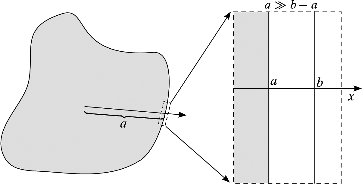
Schematic of cell membrane. The interior radius is a and the exterior is b and we assume a ≫ b – a.

4.1. Thermal Diffusion – Cell Membrane Interior

We assume that thermal transport inside the cell membrane is governed by equations (15) and (16) so that

$$\frac{\partial \left(\rho h\right)}{\partial t}+\nabla \cdot \left(\rho hv\right)=\nabla \cdot \left(k\nabla T\right).$$ (63)

We assume that the membrane is located between x = a and x = b and is thin in the geometric sense noted in Figure 3 but also in the sense of the quasi-static approximation $b-a\ll \sqrt{\kappa t^{*}}$ where κ is the thermal diffusivity k/(ρc_p) in the membrane and t* is a time scale of interest. That is, we investigate the scenario in which the time scale for thermal diffusion across the membrane (i.e. (b−a)²/κ) is much smaller than other time scales of interest in the problem⁴. This leads to the approximation ∂(ρh)/∂t ≈ 0 and thus

$$\frac{\partial \left(\rho hv\right)}{\partial x}=\frac{\partial }{\partial x}\left(k\frac{\partial T}{\partial x}\right),$$ (64)

where we have taken the fluid velocity to have the form v = (v,0,0), with v the component in the cross-membrane (x) direction. This can be integrated to give

$$\rho hv=k\frac{\partial T}{\partial x}+A_0,$$ (65)

where A₀ is independent of x. We assume that the temperature at x = a is given by T_a and the temperature at x = b is given by T_b. It then follows that

$$T=T_a+{\int }_a^x\frac{\rho hv}{k}dx+\frac{T_b-T_a}{b-a}(x-a)-\frac{x-a}{b-a}{\int }_a^b\frac{\rho hv}{k}dx.$$ (66)

Then, upon differentiation, we have

$$\frac{\partial T}{\partial x}=\frac{T_b-T_a}{b-a}+\left[\frac{\rho hv}{k}-\langle \frac{\rho hv}{k}\rangle \right],$$ (67)

where $\langle \cdot \rangle =\frac{1}{b-a}{\int }_a^b\cdot dx$ denotes the average across the membrane. Assuming that spatial gradients of the quantity ρhv/k remain bounded in the limit as b − a → 0, the quantity in brackets can be neglected when b − a is sufficiently small. Therefore, the temperature gradient is approximately constant throughout the membrane and can be expressed in terms of the temperature difference across the membrane

$$\frac{\partial T}{\partial x}=\frac{T_b-T_a}{b-a}.$$ (68)

4.2. Solute Diffusion – Cell Membrane Interior

Within the cell membrane we apply the general bulk species balance equation (6)

$$\frac{\partial c_i}{\partial t}+\nabla \cdot \left(c_{i}v\right)=-\frac{1}{M_i}\nabla \cdot J_i^{\text{B}},$$ (69)

and we suppose that $J_i^{\text{B}}$ is given by (10). Making the further assumption that the membrane is thin compared to its lateral extent (as above) and that the fluid velocity has the form v = (v, 0, 0), we have the one-dimensional equation

$$\frac{\partial c_i}{\partial t}+\frac{\partial \left(c_{i}v\right)}{\partial x}=\frac{1}{M_i}\frac{\partial }{\partial x}\left[{\mathcal{M}}_i^{\text{B}}{c}_i\frac{\partial {\mu }_i}{\partial x}\right].$$ (70)

Making a similar quasi-static argument as done in the heat transfer context with the difference now being that the time scale for chemical diffusion across the membrane is assumed fast compared to other time scales of interest⁵, we neglect the ∂c_i/∂t term, integrate once and find that

$$\frac{{\mathcal{M}}_i^{\text{B}}{c}_i}{M_i}\frac{\partial {\mu }_i}{\partial x}=c_{i}v+A_1,$$ (71)

where A₁ is independent of x.

Now suppose that ${\mu }_i={\mu }_i^a$ and ${\mu }_i={\mu }_i^b$ at x = b. Then, integrating (71), noting that ${\mathcal{M}}_i^{\text{B}}$ is not constant in general, and applying the conditions at x = a and x = b we find that

$$\begin{gathered} {\mu }_i={\mu }_i^a+M_i{\int }_a^x\frac{v}{{\mathcal{M}}_i^{\text{B}}}dx \\ +\left({\mu }_i^b-{\mu }_i^a-M_i{\int }_a^b\frac{v}{{\mathcal{M}}_i^{\text{B}}}dx\right){\left({\int }_a^b\frac{1}{{\mathcal{M}}_i^{\text{B}}{c}_i}dx\right)}^{-1}{\int }_a^x\frac{1}{{\mathcal{M}}_i^{\text{B}}{c}_i}dx. \end{gathered}$$ (72)

It then follows that

$$\frac{{\mathcal{M}}_i^{\text{B}}{c}_i}{M_i}\frac{\partial {\mu }_i}{\partial x}=\frac{1}{M_i}{\langle {\left({\mathcal{M}}_i^{\text{B}}{c}_i\right)}^{-1}\rangle }^{-1}\frac{{\mu }_i^b-{\mu }_i^a}{b-a}+c_{i}v-{\langle {\left({\mathcal{M}}_i^{\text{B}}{c}_i\right)}^{-1}\rangle }^{-1}\langle \frac{v}{{\mathcal{M}}_i^{\text{B}}}\rangle .$$ (73)

We utilize the Taylor expansion results in the supplement [14] with $f={\mathcal{M}}_i^{\text{B}}{c}_i$ and $g=v/{\mathcal{M}}_i^{\text{B}}$ and assume that f, g, ∂f/∂x and ∂g/∂x are bounded in the membrane as b − a → 0 to find

$$c_{i}v-{\langle {\left({\mathcal{M}}_i^{\text{B}}{c}_i\right)}^{-1}\rangle }^{-1}\langle \frac{v}{{\mathcal{M}}_i^{\text{B}}}\rangle =\mathcal{O}(b-a).$$ (74)

Therefore, under these assumptions we have

$$\frac{{\mathcal{M}}_i^{\text{B}}{c}_i}{M_i}\frac{\partial {\mu }_i}{\partial x}=\frac{1}{M_i}{\langle {\left({\mathcal{M}}_i^{\text{B}}{c}_i\right)}^{-1}\rangle }^{-1}\frac{{\mu }_i^b-{\mu }_i^a}{b-a}+\mathcal{O}(b-a).$$ (75)

Therefore, for a sufficiently thin membrane the flux in the membrane can be related to a difference in chemical potential across the membrane

$$J_i^{\text{B}}\cdot \widehat{n}\approx -{\langle {\left({\mathcal{M}}_i^{\text{B}}{c}_i\right)}^{-1}\rangle }^{-1}\frac{{\mu }_i^b-{\mu }_i^a}{b-a}.$$ (76)

We note that the flux forms used by Elmoazzen et al. [49] in their discussion of nondilute solvent and solute transport equations also are expressed in terms of differences in chemical potentials across the membrane. In particular, in their work the jumps in chemical potential are expressed in relation to time rates of change of the number of moles of water (N_w) and solute (N_s) in the cell [see their equations (18) and (27)].

5. Jump Conditions Across a Cell Membrane

The results of the previous section have identified forms for the thermal and chemical fluxes in the membrane under assumptions about thermal and solute diffusion time scales in the cell, membrane, and liquid regions as well as assumptions about the fluid flow within the membrane. We shall now use these results to obtain jump conditions on intra- and extracellular variables across the cell membrane. The objective is to replace a three-layer system (intracellular region, cell membrane, extracellular region) with an effective two-layer system (intracellular region, extracellular region) separated by a mathematical boundary of zero thickness representing the membrane of the cell. In the development of these results we denote the interface between the cell membrane and the intracellular region as the ‘membrane–cell interface’ and the interface between the cell membrane and the extracellular region as the ‘liquid–membrane interface’.

5.1. Mass Balance

Consider a membrane of nonzero thickness l that separates the cell interior from the liquid exterior. It follows from equation (22) that at the membrane–cell interface we have

$${\rho }^{\text{mem}}\left(v^{\text{mem}}\cdot \widehat{n}-V_{\text{n}}^{\text{mem}/\text{cell}}\right)={\rho }^{\text{cell}}\left(v^{\text{cell}}\cdot \widehat{n}-V_{\text{n}}^{\text{mem}/\text{cell}}\right),$$ (77)

where the superscript ‘mem’ indicates that the variable is defined in the membrane and is to be evaluated at the membrane–cell interface, for example, and $V_{\text{n}}^{\text{mem}/\text{cell}}$ represents the normal velocity of the membrane–cell interface. Similarly, at the liquid–membrane interface we have

$${\rho }^{\text{liq}}\left(v^{\text{liq}}\cdot \widehat{n}-V_{\text{n}}^{\text{liq}/\text{mem}}\right)={\rho }^{\text{mem}}\left(v^{\text{mem}}\cdot \widehat{n}-V_{\text{n}}^{\text{liq}/\text{mem}}\right).$$ (78)

If we assume that ρ^mem and $v^{\text{mem}}\cdot \widehat{n}$ are both constant along the direction normal to the interface and that $V_{\text{n}}^{\text{mem}/\text{cell}}=V_{\text{n}}^{\text{liq/mem}}$ so that the membrane thickness is constant, then the mass flux in the cell at the membrane is equal to the mass flux in the liquid at the membrane

$$J_{\text{mass }}:={\rho }^{\text{cell }}\left(v^{\text{cell }}-V_I\right)\cdot \widehat{n}={\rho }^{\text{liq}}\left(v^{\text{liq}}-V_I\right)\cdot \widehat{n},$$ (79)

where $V_{\text{I}}\cdot \widehat{n}=V_n^{\text{mem/cell}}=V_n^{\text{liq/mem}}$. We then interpret this equation as a ‘jump’ condition applied at a mathematically-defined boundary representing the membrane.

If we further assume that ρ^cell = ρ^liq then $v^{\text{cell}}\cdot \widehat{n}=v^{\text{liq}}\cdot \widehat{n}$ at the membrane. In fact, the density of 20% and 40% mass fraction glycerol is 1.05 and 1.1 g/mL, respectively [159], and the density of an individual cell (e.g. a leukocyte) was found to be approximately 1.08 g/mL [63], a difference of less than 3%. In this context it is useful to define the volume flux (volume of fluid per unit area per unit time) across the membrane as

$$J_{\text{vol}}=\left(v-V_{\text{I}}\right)\cdot \widehat{n}.$$ (80)

It is worth pointing out that the mass balance condition derived here does not prescribe a value to the mass/volume flux but rather a relationship between the values on either side of the membrane. We later discuss constitutive relationships for volume flux in Section 5.5 and postulate a specific one for a ternary system in Part III of this series [13].

5.2. Momentum Balance

The work of Bearman and Kirkwood [24] and Snell, Aranow and Spangler [149] on statistical mechanical descriptions of transport processes in multicomponent systems identify momentum balances for each species that involves forcing terms due to chemical potential gradients. These mixture-type models have since formed the basis for work that has investigated the role of viscosity in mass transport processes across membranes. In particular, the membrane transport theory of Mason and Viehland [111] characterizes the membrane as a spatially-fixed single component of a multicomponent mixture and arrives at a species transport equation containing, among other terms, a Darcy-type viscous term [see their equation (28)]. This model is reconciled with a variety of other transport models (e.g. the Kedem and Katchalsky model) effectively providing a common statistical mechanics interpretation. The role of viscosity in species transport and chemical reaction in a membrane was also investigated through the use of momentum balance equations in the work of Galdzicki and Miekisz [57].

The full characterization of momentum transport across a freely moving membrane should account for frictional (viscous) Darcy-type forces but also account for mechanical forces associated with membrane deformation (e.g. elasticity of the membrane). Continuum mixture theory models (e.g. Aktin and Craine [18] and Bowen [35]) offer a basis for such a description. As noted earlier, our focus in the present work is on diffusive species and thermal transport and so we do not pursue a full characterization of membrane momentum transport here.

5.3. Thermal Balance

In an analogous manner to that described above, at the membrane–cell interface we have from equation (29) that

$$k^{\text{mem}}\nabla T^{\text{mem}}\cdot \widehat{n}=k_{\text{cell}}\nabla T_{\text{cell}}\cdot \widehat{n},$$ (81)

along with the continuity of temperature T^mem = T_cell. Note that there is no latent heat effect at the membrane–cell interface. Similarly, at the membrane–liquid interface we have

$$k^{\text{mem}}\nabla T^{\text{mem}}\cdot \widehat{n}=k_{\text{liq}}\nabla T_{\text{liq}}\cdot \widehat{n},$$ (82)

and T^mem = T_liq.

Now recall the result from thermal diffusion inside the membrane that the heat flux is constant throughout the membrane

$$k^{\text{mem}}\nabla T^{\text{mem}}\cdot \widehat{n}=\frac{k^{\text{mem}}\left(T_{\text{liq}}-T_{\text{cell}}\right)}{b-a}.$$ (83)

We then have that the temperatures and heat fluxes are related across the membrane by

$$k_{\text{cell}}\nabla T_{\text{cell}}\cdot \widehat{n}=k_{\text{liq}}\nabla T_{\text{liq}}\cdot \widehat{n},$$ (84)

$$k_{\text{liq}}\nabla T_{\text{liq}}\cdot \widehat{n}=\frac{k^{\text{mem }}\left(T_{\text{liq}}-T_{\text{cell}}\right)}{b-a}.$$ (85)

If the temperature field inside the cell is uniform, it follows that $\nabla T^{\text{mem}}\cdot \widehat{n}=0$ from equation (81). In this case T_liq at the membrane–liquid interface is the same as T_cell at the membrane–cell interface. Therefore, again making the approximation that b − a is much smaller than the cell radius, equivalent boundary conditions involving only the fields in the liquid and in the cell are

$$k_{\text{liq}}\nabla T_{\text{liq}}\cdot \widehat{n}=0,$$ (86)

$$T_{\text{cell}}=T_{\text{liq}},$$ (87)

at the cell membrane.

5.4. Solute Balance

Again for a membrane of thickness b − a > 0 we have from equation (24) that at the membrane–cell interface

$$\left(c_i^{\text{mem}}-c_i^{\text{cell}}\right)V_{\text{n}}^{\text{mem}/\text{cell}}-c_i^{\text{mem}}{v}^{\text{mem}}\cdot \widehat{n}+c_i^{\text{cell}}{v}^{\text{cell}}\cdot \widehat{n}=-\frac{1}{M_i}{J}_i^{\text{B}\left(\text{cell}\right)}\cdot \widehat{n}+\frac{1}{M_i}{J}_i^{\text{B}\left(\text{mem}\right)}\cdot \widehat{n}.$$

Similarly, at the liquid–membrane interface we have

$$\left(c_i^{\text{liq}}-c_i^{\text{mem}}\right)V_{\text{n}}^{\text{liq}/\text{mem}}-c_i^{\text{liq}}{v}^{\text{liq}}\cdot \widehat{n}+c_i^{\text{mem}}{v}^{\text{mem}}\cdot \widehat{n}=-\frac{1}{M_i}{J}_i^{\text{B}\left(\text{mem}\right)}\cdot \widehat{n}+\frac{1}{M_i}{J}_i^{\text{B}\left(\text{liq}\right)}\cdot \widehat{n}.$$

At the membrane–cell interface we have $c_i^{\text{mem}}={\Phi }_i{c}_i^{\text{cell}}$ and at the liquid–membrane interface we have $c_i^{\text{mem}}={\Phi }_i{c}_i^{\text{liq}}$ where Φ_i are partition coefficients associated with species i and the membrane (see Stein [152], or Friedman [52], and also Wijmans and Baker [166] who have a similar relationship between concentrations on either side of a membrane related to a ‘sorption’ coefficient that is the ratio of activity coefficients outside and inside the membrane). Using these and equation (76) along with the assumption that $V_{\text{n}}^{\text{mem}/\text{cell}}=V_{\text{n}}^{\text{liq/mem}}=V_{\text{I}}\cdot \widehat{n}$ we find that at the membrane–cell interface

$$\left({\Phi }_i-1\right)c_i^{\text{cell}}{V}_{\text{I}}\cdot \widehat{n}-{\Phi }_i{c}_i^{\text{cell}}{v}^{\text{mem}}\cdot \widehat{n}+c_i^{\text{cell}}{v}^{\text{cell}}\cdot \widehat{n}=-\frac{1}{M_i}{J}_i^{\text{B}\left(\text{cell}\right)}\cdot \widehat{n}-\frac{{\langle {\left({\mathcal{M}}_i^{\text{B}}{c}_i^{\text{mem}}\right)}^{-1}\rangle }^{-1}\Delta {\mu }_i}{l{M}_i}$$ (88)

where $\Delta {\mu }_i={\mu }_i^{\text{liq}}-{\mu }_i^{\text{cell}}$ and l = b − a is the membrane thickness. Similarly, at the membrane–liquid boundary

$$\left(1-{\Phi }_i\right)c_i^{\text{liq}}{V}_{\text{I}}\cdot \widehat{n}+{\Phi }_i{c}_i^{\text{liq}}{v}^{\text{mem}}\cdot \widehat{n}-c_i^{\text{liq}}{v}^{\text{liq}}\cdot \widehat{n}=\frac{{\langle {\left({\mathcal{M}}_i^{\text{B}}{c}_i^{\text{mem}}\right)}^{-1}\rangle }^{-1}\Delta {\mu }_i}{l{M}_i}+\frac{1}{M_i}{J}_i^{\text{B}\left(\text{liq}\right)}\cdot \widehat{n}.$$ (89)

Rewriting these using the mass balance results given in Eq. (79) gives

$$-{\Phi }_i{c}_i^{\text{cell}}\frac{J_{\text{mass}}}{{\rho }^{\text{mem}}}+c_i^{\text{cell}}\frac{J_{\text{mass}}}{{\rho }^{\text{cell}}}=-\frac{1}{M_i}{J}_i^{\text{B}\left(\text{cell}\right)}\cdot \widehat{n}-\frac{{\langle {\left({\mathcal{M}}_i^{\text{B}}{c}_i^{\text{mem }}\right)}^{-1}\rangle }^{-1}\Delta {\mu }_i}{l{M}_i},$$ (90)

and

$${\Phi }_i{c}_i^{\text{liq}}\frac{J_{\text{mass}}}{{\rho }^{\text{mem}}}-c_i^{\text{liq}}\frac{J_{\text{mass}}}{{\rho }^{\text{liq}}}=\frac{{\langle {\left({\mathcal{M}}_i^{\text{B}}{c}_i^{\text{mem}}\right)}^{-1}\rangle }^{-1}\Delta {\mu }_i}{l{M}_i}+\frac{1}{M_i}{J}_i^{\text{B}\left(\text{liq}\right)}\cdot \widehat{n}.$$ (91)

Under the further assumption that ρ^cell = ρ^mem = ρ^liq these equations reduce (using Eq. (80)) to

$$\left(1-{\Phi }_i\right)c_i^{\text{cell}}{J}_{\text{vol}}=-\frac{1}{M_i}{J}_i^{\text{B}\left(\text{cell}\right)}\cdot \widehat{n}-\frac{{\langle {\left({\mathcal{M}}_i^{\text{B}}{c}_i^{\text{mem}}\right)}^{-1}\rangle }^{-1}\Delta {\mu }_i}{l{M}_i},$$ (92)

and

$$-\left(1-{\Phi }_i\right)c_i^{\text{liq}}{J}_{\text{vol}}=\frac{{\langle {\left({\mathcal{M}}_i^{\text{B}}{c}_i^{\text{mem}}\right)}^{-1}\rangle }^{-1}\Delta {\mu }_i}{l{M}_i}+\frac{1}{M_i}{J}_i^{\text{B}\left(\text{liq}\right)}\cdot \widehat{n}.$$ (93)

We shall simplify these further in the ternary case in Part III of this series [13] and there postulate a constitutive law for the volume flux J_vol. Some general discussion of this volume flux is given in the next section.

5.5. Constitutive Law for Volume Flux Across Membrane

In general, one must also provide a constitutive law for the volume flux across the membrane. There are a number of existing models for solute and solvent transport through biological membranes (although as argued in Section 5.2 transport models have been derived from the analysis of momentum transport models using statistical mechanical theories [111] and [57]). For thorough reviews of these models we refer the reader to the work of Kleinhans [83] and Elmoazzen et al. [49]. We briefly summarize two well-known models – the two-parameter (2P) formalism and the Kedem–Katchalsky (KK) formalism – and explain the relation of the present model to those as well as to the nondilute transport model outlined by Elmoazzen et al. The 2P and KK formalisms can be distinguished by the type of channels assumed present in the membrane that can transport solute and/or solvent. In the 2P formalism it is assumed that solute and solvent are transported selectively through separate channels in the membrane. For example, aquaporins are water-selective channels that appear in a variety of animal and plant cells [83]. The 2P formalism owes its name to each process (water and solute transport) having associated with it its own permeability parameter (typically the hydraulic conductivity L_p and solute permeability P_s). The KK formalism addresses the case in which solvent and solute transport across the membrane are coupled – e.g. when solute and solvent transport occur through a common (cotransporting) channel. In addition to solute and solvent permeability parameters the KK formalism also introduces the so-called reflection coefficient to account for this coupling. Both Kleinhans and Elmoazzen et al. make comparisons between the 2P and KK formalisms. Kleinhans argues that for cases in which cotransporting channels are absent the two models agree; Elmoazzen et al. demonstrate that the total volume fluxes are identical in this limit. The 2P and KK formalisms have been generalized to allow for the presence of multiple types of transport pathways—e.g. cotransporting channels along with selective ones allowing only solute or solvent transport (see Kleinhans [83]). These models are commonly used in the dilute solution limit. The work of Elmoazzen et al. extends the 2P description by identifying solute and solvent transport equations for the non-dilute limit.

6. Discussion and Conclusions

In Part I of the series, we developed the foundations of the transport models used in the present manuscript. Applying these foundational models is fairly simple in the case of bulk solutions, but as is the case with many differential equation models, the challenges occur at the boundaries. In particular, the reason why the bulk case is simple is because of the Transport Theorem described in Part I, which addresses energy or mass conservation by assuming an arbitrary domain away from boundaries. Once near a boundary, however, one must address the conservation of all relevant quantities on a case-by-case basis. When the boundaries are moving, and especially when their movement is dependent on the governing equations (e.g. the boundary of a moving piston may be a priori addressed by reparameterization of the domain as a function of piston placement), even more care must be taken. Our present system is a cell surrounded by media with an encroaching solidification front and contains a number of coupled domains, specifically, the extracellular solid and liquid, the cell membrane, and intracellular spaces, each with a set of interfacial and boundary conditions that is dependent on the state of the neighboring domain. As described in detail in Part I, classical models used in cryobiology have made varying simplifications of these different domains. For example, many treatments of cells in freezing media assume no spatial concentration gradients anywhere, save for the solid-liquid interface where it is assumed that solutes are uniformly rejected (i.e. K₀ = 0) [114]. Other treatments have carefully addressed extracellular concentration gradients during cryo-protocols, but have assumed that the solute polarization effects at both sides of a cell membrane are negligible [2, 40]. Others, have looked at the effect of solute polarization at the membrane [98, 99, 101, 102] but not in conjunction with solute polarization at the solid-liquid interface. Others have looked at the effects of solute polarization at the solidifying ice front [85, 86]. Here we have attempted to combine elements of all of these treatments in a general setting that does not dictate the specifics of chemical potential or domain shape. In fact, this demonstrates the power of generality, as we will then be able to make choices about the necessity of specific chemical potential models (some of which were discussed in Part I of this series), as well as the shape of the domain. In particular, in Part III we will choose a fairly simple chemical potential model and a spherically symmetric domain to demonstrate the pieces of the model with reduced analytical and numerical complication.

In the present system we also attempt to include a number of liquid-solute interfacial effects. In particular, the melting temperature or freezing point depression at the interface is particularly relevant to a system undergoing solidification and is a function of a number of different quantities including composition, pressure, curvature, and interfacial velocity. Our treatment of the pressure dependence of melting temperature includes the classical approach considering only pure solvents. This approach, for example, is used to derive the model used by Mazur [114] and a number of follow up papers, and allows the expression of melting temperature explicitly as a function of pressure and the relative densities of the liquid and solid components. Our work, however, also includes treatment of multisolute pressure effects on interfacial melting temperature. We demonstrate that melting point predictions may be made by considering the appropriate thermodynamic model and its components. This is in contrast to the purely phenomenological model of Guignon et al. [66], which may be sufficient for many specific instances, but has drawbacks that include the necessity of the determination of the set of parameters for each application. However, it is important to note that Guignon et al. demonstrate that the interaction between concentration and pressure plays a minimal role in freezing point depression. A more careful thermodynamic analysis of the Gibbs-Duhem derived multisolute Clapeyron equation in the context of cryobiology is warranted.

Curvature effects have been examined in the cryobiological literature, for example, with applications to ice propagation through capillary straws [105] and through membrane pores [3]. We noted in our derivation that under an assumption of a spherically symmetric ice front with a diameter larger than a cell, the melting point depression will be minimal. These effects may prove to be important in unstable solidification fronts where neighboring points can take on positive and negative curvatures, amplifying the effect [46]. In Part III we make the simplifying assumption that the ice front is, in fact, spherical, and therefore this effect will be minimized.

We also presented a classical but careful treatment of transport through a membrane, showing that spatial and temporal scale arguments can be used to reduce the spatially dependent intramembrane transport model to one containing only conditions at the membrane boundaries. While this is a typical argument, the utility and accuracy of the underlying assumptions are dependent on the underlying model. In particular, if the transport is, as assumed here, diffusive, then our approach is appropriate. If the transport is active, with membrane pores selectively and actively transporting water and solutes, then more care must be taken.

In this manuscript we have carefully derived the critical heat and mass transport equations for a general system containing a cell in liquid media surrounded by an ice front. We have shown how to use length and time-scale arguments to treat the cell membrane as an abstract, zero-thickness, interface using jump conditions. We have discussed multiple mechanisms for the critical prediction of depression of the freezing point of the surrounding media and coupled this to the rate at which the ice front moves. In the third part of this series, we proceed with our model in the specific context of a ternary system, identify a form for the volume flux appropriate for this case and present computational results for the case of inward solidification of a ternary mixture towards a spherical biological cell.