Sensitivity of Cross-Trained Deep CNNs for Retinal Vessel Extraction

Abstract

Automatic segmentation of vascular network is a critical step in quantitatively characterizing vessel remodeling in retinal images and other tissues. We proposed a deep learning architecture consists of 14 layers to extract blood vessels in fundoscopy images for the popular standard datasets DRIVE and STARE. Experimental results show that our CNN characterized by superior identifying for the foreground vessel regions. It produces results with sensitivity higher by 10% than other methods when trained by the same data set and more than 1% with cross training (trained on DRIVE, tested with STARE and vice versa ) . Further, our results have better accuracy > 0.95% compared to state of the art algorithms.

I. INTRODUCTION

Segmentation and quantification of the vascular tree in retinal images is substantial for diagnosing some serious diseases such as diabetic, glaucoma, macular degeneration and hypertension. Early diagnosis for those diseases can decrease the risk of blindness and vision loss. Manual segmentation is tedious, time and effort consuming as it needs experienced specialists to manually annotate the vessel. Recently, many automated algorithms and methods for thin structure segmentation have been proposed in the literature. These algorithms can fit in to two categories, either supervised or unsupervised. In supervised algorithms [1]–[9], a training set with the corresponding ground truth enables the classifier to learn the rules in how to discriminate between the foreground versus background. Whereas unsupervised algorithms [10]–[19] depends upon other techniques such as applying filters, tracking and model-based approaches without the need to labeled data. Challenges in those images such as contrast variation, illumination artifacts, irregular optic disk, curvy thin vessels and central reflux make vascular tree extraction as a vital and challenged problem to researchers. Recently deep learning networks provide the state of the art results in terms of segmentation and classification, however, the limited number of annotated data in biomedical application still considered as a bottleneck for these types of problems. Regardless of that, there are some papers in the literature [8], [9], [20] that give a promising results compared to traditional methods.

Rest of the paper is organized as follows. Section II describes our proposed CNN architecture and the details for training and testing, Section III describe the datasets and the evaluation methods, Section IV provides detailed experimental results on retinal imagery of DRIVE and STARE data sets, and finally conclusions in Section V.

II. CONVOLUTIONAL NEURAL NETWORK(CNN) FOR RETINAL IMAGES

Traditional hand-crafted features and matched filtered techniques may fail to obtain an accurate detection for the vascular tree especially for the tiny vessels located within high contrast variations. Deep learning has been very famous in solving problems. CNN composed of a set of hidden layers (convolution, ReLU and pooling) that accept the image as input and produce confidence map as output. Stochastic gradient descent (SGD) with back propagation mostly used to update the parameters. Convolution followed by ReLU and pooling enables the network to find a suitable set of features that efficiently characterize any dataset. Forward and back propagation for several epochs is enough to learn the high representation of the objects in the image.

A. Proposed CNN architecture

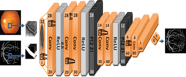
The proposed CNN architecture built on top of MatConvNet [21]. The linear structure of the vessels doesn’t require a very deep network since the higher representation of the vessels will ultimately vanished. Also, narrow network with small number of layers is not enough to capture and produce efficient feature maps to represent the vessels. This network has been designed after extensive trials for different configurations. We haven’t begun designing the network from scratch such as [8] in which they built a narrow network with just 3 hidden layers or [9] who has different configurations designed from scratch. We began our network trials with a model designed for mnist digits classification in MatConvNet since vessels have similar linear structures. Then we tuned the parameters and add layer by layer until we get best accuracy. Our network consists of 9 convolution layers, 3 ReLU, 2 pooling and one softmax layer to discriminate between classes. Figure 1 visualize the network. Our CNN accepts patches with size 32 × 32 as input, filters are convolved with the input image to produce feature maps, filter size begins with 5×5 and then dimension decreases to 3×3 in the last layers. The last two layers are fully connected layers to produce the probability map to identify the pixels or patches as vessels versus no vessels.

Fig. 1.

The proposed CNN configuration: numbers at the top represent the dimension of the patch, numbers at the bottom represent feature maps dimension, layers are either convolution, pooling or ReLU, filter size is (5×5) for the first 7 layers, (3×3) for the next 5 layers and the last two layers are fully connected, output is either F (foreground) or G (background).

B. Training and testing using our CNN

Machine learning algorithms need to be trained first to learn the weights that identify the classes. Vessels have just two classes, foreground (vessel) and background (non-vessel). The network has been learned using sets of patches extracted from our input images. The extracted patches have dimension equal to 32×32 from the second channel. The green channel usually has most of the valuable information in terms of color and structure. Also using just one channel significantly increases the speed of the training process. After training the model with specific number of epochs with min-batch SGD, the weights will be optimized to recognize the vessels. In testing phase, the network tested with totally different set of images by two procedures:

1. Testing with overlapping patches: Overlapping patches are extracted from the image to be tested on the network. The trained CNN will decide whether the patch is vessel or non-vessel. This procedure will produce a smooth linear structure since each patch correspond to one pixel in the output image, however, it is computationally expensive, It takes about 15 minutes to segment the whole image.

2. Testing the full image: The green channel of the full image becomes the input to the network, decrease in size layer by layer until the end of the model. Ultimately, up-sampling is used to return the image to its original size with FG vs BG pixel based classification. This approach is very fast and needs just one second to predict the whole image, whoever, it is less precise.

III. DATA SET AND EVALUATION METHODS

The experiments were performed on two publicly famous data sets: DRIVE and STARE. DRIVE¹ stands for Digital Retinal Images for Vessel Extraction which consists of 20 images for training and different 20 for testing. STARE data set stands for STructured Analysis of the Retina² consists of 20 images for both training and testing. We evaluated our results using the standard metrics that usually used for evaluation: Sensitivity(Se), Specificity(Sp) and Accuracy(Acc).

$$\begin{array}{l}Sensitivity=\frac{TP}{TP+FN},Specificity=\frac{TN}{TN+FP},\\ Accuracy=\frac{TP+TN}{TP+FP+FN+TN}\end{array}$$

where TP stands for true positive, TN for true negative, FP for false positive and FN for false negative.

IV. EXPERIMENTAL RESULTS AND DISCUSSION

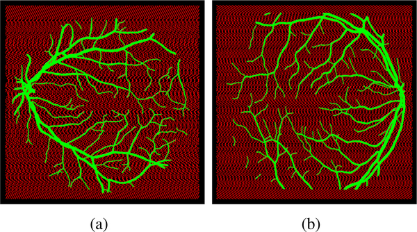
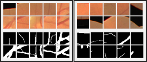
The experiments performed on retinal images for both DIRVE and STARE data sets. Weights were initialized randomly, updated iteratively by SGD and back propagation with min-batch equal to 100 for 24 epochs. Further, we trained the network with approximately equal number of positive and negative cases to prevent the classifier to be biased to one of the classes. In the training phase, patches are extracted from the input images with stride equal to 1 and 12 for foreground and background respectively, see figure 3 for better visualization. Any patch considered as a vessel if it passes through the center of the patch, see figure 2. In case of DRIVE data set, the training set is constructed using the 20 images available for training. The dimension for each image is 565×584 that form a training set consists of 1121951 patches. For the STARE data set, Leave one out cross validation has been used to train the network. In each experiment, 19 images are used for training and 1 for testing, the dimension of each image is 605×700 corresponds to 1304940 observations. Table I summarizes the data base statistics used to train our model. Table II compares overlapping image patches versus full image segmentation with postprocessing (P) and thinning (T). Further, it compares testing the data of DRIVE using the trained model of STARE data set and vice versa to show how our model is robust toward capturing the vessels even with different data set. There are six experiments related to the two procedures discussed in II-B. In the first three experiments, overlapping patches from the images are considered as input. The first set of results indicated by (Overlap patch) are the predicted results without any post processing, the second set (Overlap patch + P) after morphological cleaning for spurious results using structural element equal to 100. The third experiment (Overlap patch + P + T) is with thinning. In the second set of experiments, we applied the learned filter coefficients on the full image as input, dimension decreases layer by layer to produce probability map with dimension 142×147 and 152×176 for DRIVE and STARE respectively. Up-sampling is used to return the image to it’s original size. From table II, the set of values with the highest accuracy considered as final results to compare with other algorithms in the literature. In tables III and IV, we observe that our algorithm characterized by its robust detection which outperform other state of the art methods. In the two data sets, sensitivity is 0.8789 and 0.8600 which is approximately 10% higher than other algorithms in the literature. additionally, our algorithm produces better accuracy in both data sets with comparable specificity. Also it is interesting to see that our CNN results has higher sensitivity and accuracy even with cross training which make the network to be considered as a promising architecture that can be used to segment other similar data sets.

Fig. 3.

Visualization of the trained patches, green dots represent positive cases, red dots represent negative cases: (a) image with id#01 in DRIVE dataset superimposed on the corresponding GT with overlapping foreground pixels equal to 24658 and background patches equal to 27964 with stride equal to 12 instead of 77059 when stride equal 1, (b) image number id#82 in the STARE data set superimposed on the GT with overlapping foreground pixels equal to 33310 and background patches equal to 35710 with stride equal to 12 instead of 392804 with overlapping patches

Fig. 2.

Examples of positive cases (left), and negative cases (right), the patch considered foreground if the vessel pass across the center of the patch

TABLE I.

EXPERIMENT STATISTICS

Data set	DRIVE		STARE
Dimention	565×584		605×700
Training scheme	train 20, test 20		Leave one out
Total no of patches	1,121,951		1,304,940
	FG	BG	FG	BG
Patches no.	569,615	552,336	625,808	679,132
Stride	1	12	1	12

TABLE II.

PERFORMANCE RESULTS USING THE PROPOSED CNN, COMPARING OVERLAPPING IMAGE PATCHES VERSUS FULL IMAGE SEGMENTATION WITH POSTPROCESSING (P) AND THINNING (T) TO REFINE VESSEL BOUNDARIES, FOR BOTH DRIVE AND STARE.

{Dataset}	Training DRIVE Testing DRIVE			Training DRIVE Testing STARE			Training STARE Testing STARE			Training STARE Testing DRIVE
Evaluation	Se	Sp	Acc	Se	Sp	Acc	Se	Sp	Acc	Se	Sp	Acc
Overlap patch	0.9128	0.9463	0.9432	0.9094	0.9325	0.9309	0.9824	0.9197	0.9246	0.8307	0.9598	0.9483
Overlap patch + P	0.8981	0.9563	0.9510	0.9056	0.9407	0.9382	0.9801	0.9377	0.9411	0.8098	0.9683	0.9542
Overlap patch + P + T	0.8789	0.9606	0.9533	0.7841	0.9749	0.9606	0.8600	0.9754	0.9667	0.7953	0.9708	0.9552
Full Image	0.7522	0.9446	0.9276	0.7539	0.9257	0.9136	0.8346	0.8999	0.8949	0.6559	0.9253	0.9016
Full Image + P	0.7300	0.9499	0.9306	0.7273	0.9397	0.9247	0.8196	0.9221	0.9142	0.5927	0.9541	0.9224
Full Image + P + T	0.6105	0.9719	0.9402	0.6167	0.9656	0.9401	0.6667	0.9319	0.9538	0.5806	0.9562	0.9233

V. CONCLUSIONS

We proposed a CNN configuration that can extract the vascular tree in retinal images. Our network characterized by it’s robust detection toward capturing the small vessels. It produces significantly better segmentation results in sensitivity (> 0.86) and accuracy (> 0.95) compared to the state of the art algorithms in the literature. Further, it is a robust network even with cross training as there is only (8%) difference in sensitivity compared to normal training. Our promising results can then be quantified to recognize the morphological attributes of blood vessels.

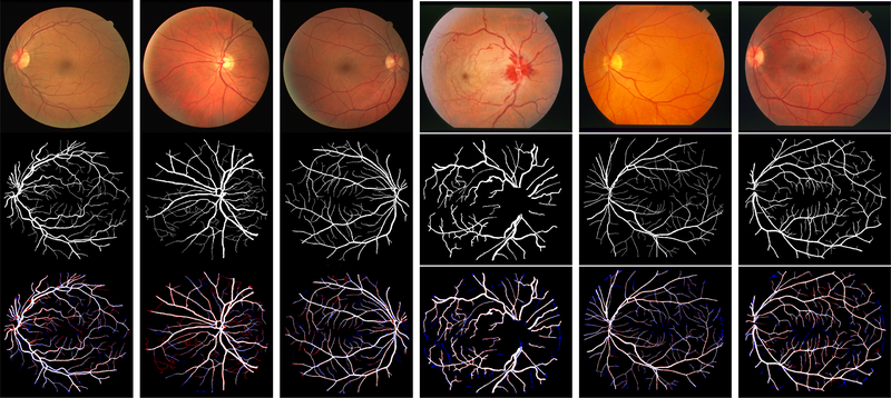
Fig. 4.

Our patch-based deep learning segmentation obtains robust results when applied directly to retinal images for DRIVE and STARE dataset, first row represents the raw images with ids (#01, #11, #14, #0005, #0162, #0255) , second row represents the ground truth and our robust prediction is shown in the third row. red are missing (false negative) and blue are extra regions (false positive) compared to ground truth

TABLE III.

COMPARISON WITH STATE OF THE ART METHODS ON DRIVE

No	Methods	Year	Se	Sp	Acc
1	Zana [11]	2001	0.6971	N.A	0.9377
2	Jiang [12]	2003	N.A	N.A	0.9212
3	Niemeijer [1]	2004	N.A	N.A	0.9416
4	Staal [3]	2004	N.A	N.A	0.9441
5	Mendonca [13]	2006	0.7344	0.9764	0.9452
6	Soares [2]	2006	0.7332	0.9782	0.9461
8	Al-Diri [14]	2009	0.7282	0.9551	N.A
9	Lam [15]	2010	N.A	N.A	0.9472
10	Miri [16]	2011	0.7352	0.9795	0.9458
11	Fraz [17]	2011	0.7152	0.9759	0.9430
12	You [18]	2011	0.7410	0.9751	0.9434
13	Marin [5]	2011	0.7067	0.9801	0.9452
14	Fraz [6]	2012	0.7406	0.9807	0.9480
15	Cheng [7]	2014	0.7252	0.9798	0.9474
16	Azzopardi [19]	2015	0.7655	0.9704	0.9442
17	Li [8]	2016	0.7569	0.9816*	0.9527
18	Liskowski [9]	2016	0.7763	0.9768	0.9495
19	Zhang [10]	2016	0.7743	0.9725	0.9476
20	Ours	2018	0.8789*	0.9606	0.9533
21	Ours (Cross trained)	2018	0.7953	0.9708	0.9552*

^*. WITH BOLD DENOTE THE BEST VALUE, ONLY BOLD REFER TO THE SECOND BEST VALUE IN COMPARISON

TABLE IV.

COMPARISON WITH STATE OF THE ART METHODS ON STARE.

No	Methods	Year	Se	Sp	Acc
1	Hoover [22]	2000	0.6747	0.9565	0.9264
2	Jiang [12]	2003	N.A	N.A	0.9009
3	Staal [3]	2004	N.A	N.A	0.9516
4	Mendonca [13]	2006	0.6996	0.9730	0.9440
5	Soares [2]	2006	0.7207	0.9747	0.9479
6	Ricci [4]	2007	N.A	N.A	0.9584
7	Al-Diri [14]	2009	0.7521	0.9681	N.A
8	Lam [15]	2010	N.A	N.A	0.9567
9	Fraz [17]	2011	0.7311	0.9680	0.9442
10	You [18]	2011	0.7260	0.9756	0.9497
11	Fraz [6]	2012	0.7548	0.9763	0.9534
12	Azzopardi [19]	2015	0.7716	0.9701	0.9563
13	Li [8]	2016	0.7726	0.9844*	0.9628
14	Liskowski [9]	2016	0.7620	0.9789	0.9571
15	Zhang [10]	2016	0.7791	0.9758	0.9554
16	Ours	2018	0.8600*	0.9754	0.9667*
17	Ours (Cross trained)	2018	0.7841	0.9749	0.9606

REFERENCES

- [1].Niemeijer M, Staal J, van Ginneken B, Loog M, and Abramoff MD, “Comparative study of retinal vessel segmentation methods on a new publicly available database,” Medical Imaging 2004: Image Processing, vol. 5370, pp. 648–656, 2004. [Google Scholar]
- [2].Soares JVB, Leandro JJG, Cesar RM, Jelinek HF, and Cree MJ, “Retinal vessel segmentation using the 2d gabor wavelet and supervised classification,” IEEE Trans. Med. Imag, vol. 25, no. 9, pp. 1214–1222, 2006. [DOI] [PubMed] [Google Scholar]
- [3].Staal J, Abramoff MD, Niemeijer M, Viergever MA, and van B Ginneken, “Ridge-based vessel segmentation in color images of the retina.,” IEEE Trans. Med. Imaging, vol. 23, no. 4, pp. 501–509, 2004. [DOI] [PubMed] [Google Scholar]
- [4].Ricci E. and Perfetti R, “Retinal blood vessel segmentation using line operators and support vector classification,” IEEE Transactions on Medical Imaging, vol. 26, no. 10, pp. 1357–1365, 2007. [DOI] [PubMed] [Google Scholar]
- [5].Maŕın D, Aquino A, Gegundez-Arias ME, and Bravo JM, “A new´ supervised method for blood vessel segmentation in retinal images by using gray-level and moment invariants-based features,” IEEE Transactions on medical imaging, vol. 30, no. 1, pp. 146–158, 2011. [DOI] [PubMed] [Google Scholar]
- [6].Fraz MM, Remagnino P, Hoppe A, Uyyanonvara B, Rudnicka AR, Owen CG, and Barman SA, “An ensemble classification-based approach applied to retinal blood vessel segmentation,” IEEE Transactions on Biomedical Engineering, vol. 59, no. 9, pp. 2538– 2548, 2012. [DOI] [PubMed] [Google Scholar]
- [7].Cheng EK, Du L, Wu Y, Zhu YJ, Megalooikonomou V, and Ling HB, “Discriminative vessel segmentation in retinal images by fusing context-aware hybrid features,” Machine Vision and Applications, vol. 25, pp. 1779–1792, 2014. [Google Scholar]
- [8].Li Q, Feng B, Xie L, Liang P, Zhang H, and Wang T, “A crossmodality learning approach for vessel segmentation in retinal images,” IEEE Trans. Med. Imag, vol. 35, no. 1, pp. 109–118, 2016. [DOI] [PubMed] [Google Scholar]
- [9].Liskowski P. and Krawiec K, “Segmenting retinal blood vessels with deep neural networks,” IEEE Trans. Medical Imag, vol. 35, no. 11, pp. 2369–2380, 2016. [DOI] [PubMed] [Google Scholar]
- [10].Zhang J, Dashtbozorg B, and Bekkers E, “Robust retinal vessel segmentation via locally adaptive derivative frames in orientation scores,” IEEE Transactions on Medical Imaging, vol. 35, no. 12, pp. 2631 – 2644, 2016. [DOI] [PubMed] [Google Scholar]
- [11].Zana F. and Klein JC, “Segmentation of vessel-like patterns using mathematical morphology and curvature evaluation,” IEEE Transactions on Image Processing, vol. 10, pp. 1010–1019, 2001. [DOI] [PubMed] [Google Scholar]
- [12].Jiang X. and Mojon D, “Adaptive local thresholding by verification-based multithreshold probing with application to vessel detection in retinal images,” IEEE Transactions on Pattern Analysis and Machine Intelligence, vol. 25, no. 1, pp. 131–137, 2003. [Google Scholar]
- [13].Mendonca AM and Campilho A, “Segmentation of retinal blood vessels by combining the detection of centerlines and morphological reconstruction,” IEEE Transactions on Medical Imaging, vol. 25, no. , pages=1200–1213, year=2006, DOI = ””,. [DOI] [PubMed] [Google Scholar]
- [14].Al-Diri B, Hunter A, and Steel D, “An active contour model for segmenting and measuring retinal vessels,” IEEE Transactions on Medical Imaging, vol. 28, no. 9, pp. 1488–1497, 2009. [DOI] [PubMed] [Google Scholar]
- [15].Lam BSY, Gao YS, and Liew AWC, “General retinal vessel segmentation using regularization-based multiconcavity modeling,” IEEE Transactions on Medical Imaging, vol. 29, pp. 1369–1381, 2010. [DOI] [PubMed] [Google Scholar]
- [16].Miri MS and Mahloojifar A, “Retinal image analysis using curvelet transform and multistructure elements morphology by reconstruction,” IEEE Transactions on Biomedical Engineering, vol. 58, pp. 1183– 1192, 2011. [DOI] [PubMed] [Google Scholar]
- [17].Fraz MM, Barman SA, Remagnino P, Hoppe A, Basit A, Uyyanonvara B, Rudnicka AR, and Owen CG, “An approach to localize the retinal blood vessels using bit planes and centerline detection,” Computer Methods and Programs in Biomedicine, vol. 108, no. 2, pp. 600–616, 2012. [DOI] [PubMed] [Google Scholar]
- [18].You XG, Peng QM, Yuan Y, Cheung YM, and Lei JJ, “Segmentation of retinal blood vessels usingthe radial projection and semi-supervised approach,,” . [Google Scholar]
- [19].Azzopardi G, Strisciuglio N, Vento M, and Petkov N, “Trainable cosfire filters for vessel delineation with application to retinal images,” Med. Image Anal, vol. 19, no. 1, pp. pp. 46–57, 2015. [DOI] [PubMed] [Google Scholar]
- [20].Kassim YM, Prasath VBS, , Glinskii Olga V., Glinsky Vladislav V., Huxley Virginia H., and Palaniappan K, “Microvasculature segmentation of arterioles using deep cnn,” in IEEE International Conference on Image Processing, Beijing, China, 2017. [Google Scholar]
- [21].Vedaldi A. and Lenc K, “MatConvNet: Convolutional neural networks for MATLAB,” pp. 689–692, 2015. [Google Scholar]
- [22].Hoover A, Kouznetsova V, and Goldbaum M, “Locating blood vessels in retinal images by piecewise threshold probing of a matched filter response,” IEEE Transactions on Medical Imaging, vol. 19, pp. 203–210, 2000. [DOI] [PubMed] [Google Scholar]