Dynamics analysis of a delayed virus model with two different transmission methods and treatments

Abstract

In this paper, a delayed virus model with two different transmission methods and treatments is investigated. This model is a time-delayed version of the model in (Zhang et al. in Comput. Math. Methods Med. 2015:758362, 2015). We show that the virus-free equilibrium is locally asymptotically stable if the basic reproduction number is smaller than one, and by regarding the time delay as a bifurcation parameter, the existence of local Hopf bifurcation is investigated. The results show that time delay can change the stability of the endemic equilibrium. Finally, we give some numerical simulations to illustrate the theoretical findings.

Introduction and model formulation

Infectious diseases are still important diseases that endanger human health [2]. Not only do some ancient infectious disease pathogens continue to mutate and change, but new pathogens are also emerging, bringing many difficulties for us to discover, diagnose, and prevent infectious diseases. Studies have shown that many diseases are caused by viruses. Of more than 4000 viruses discovered so far, more than 100 can directly threaten human health and life. For example, rabies, a zoonotic disease caused by rabies virus, can cause severe encephalitis. Because the virus invades the central nervous system, if the treatment is not taken in time, the mortality rate is almost 100%. Another example is the Ebola virus, which causes Ebola hemorrhagic fever with a mortality rate from 50% to 90%. In addition, recent research has shown that several viruses have been found to link with cancer in humans, even that can push the cell toward becoming cancerous, such as human papilloma viruses (HPVs) which are considered to be the biggest factor that causes various cancers such as cervical cancer [3–5], anal cancer [6, 7], and oropharyngeal cancers [8]. The sudden outbreak of the SARS virus and the Ebola virus in the past 20 years has given us a major warning that public health issues are no longer just health issues, but also an important part of national security and urban security systems.

Using mathematical models to help discover the mechanism of viral transmission to predict the development of infectious diseases has become the mainstream method for controlling and preventing infectious diseases [9–12]. Therefore, for over a century, lots of mathematical models have been established to explain the evolution of the free virus in a body, and mathematical analysis was implemented to explore the threshold associated with eradication and persistence of the virus; for example, [13–16] studied the global dynamic behavior of HIV models, [17–24] analysed the global dynamics of HBV models [25–28]. A general class of models describing the process of virus invading the target cells and release of the virus due to the infected cell apoptosis has been established and analyzed by Perelson et al. [29, 30] and Nelson et al. [31] as follows:

$$\{\begin{array}{c}\frac{dx}{dt}=\Lambda -dx-\alpha vx,\hfill \\ \frac{dy}{dt}=\alpha vx-ay,\hfill \\ \frac{dv}{dt}=ky-uv,\hfill \end{array}$$ 1

where x, y, and v represent the concentrations of uninfected target cells, infected cells, and virus, respectively. Λ and d are the generation rate and mortality rate of uninfected target cells respectively, α is the infection rate, a is the mortality rate of infected cells, k and u are the generation rate and mortality rate of free virus respectively.

However, the above model only considers that free viruses can infect uninfected cells by direct contact with them. Recent studies have shown that virus can be transmitted directly from cell to cell by virological synapses, i.e., cell-to-cell transmission [32–39]. Spouge et al. [40] built a model to characterize this phenomenon:

$$\{\begin{array}{c}\frac{dC}{dt}=r_{C}C(1-\frac{C+I+\gamma M}{C_m})-k_{I}IC,\hfill \\ \frac{dI}{dt}=k_{I}IC-{\mu }_{I}I,\hfill \\ \frac{dM}{dt}={\mu }_{C}C+{\mu }_{I}I,\hfill \end{array}$$ 2

where C, I, M represent the concentrations of uninfected cells, infected cells, and dead cells, respectively. $k_I$ is the rate constant for cell-to-cell spread, $r_C$ is the reproductive rate of uninfected cell. ${\mu }_I$, ${\mu }_C$ are the rate constants at which uninfected or infected cells die respectively, and the term $k_{I}IC$ represents the cell-to-cell transmission. However, research [41] shows that there is a delay between the time an uninfected cell becomes infected and when it begins to infect other uninfected cells, then Culshaw et al. [42] improved the model by introducing a distributed delay into model (2) and got the following model:

$$\{\begin{array}{c}\frac{dC}{dt}=r_{C}C(t)(1-\frac{C(t)+I(t)}{C_M})-k_{I}C(t)I(t),\hfill \\ \frac{dI}{dt}=k_I^{\prime }{\int }_{-\mathrm{\infty }}^{t}C(u)I(u)F(t-u)du-{\mu }_{I}I(t),\hfill \end{array}$$

where $F(u)$ is the delay kernel.

Lai et al. [43] proposed a model containing two different types of infection as follows:

$$\{\begin{array}{c}\frac{dT}{dt}=rT(t)(1-\frac{T(t)+\alpha T^{\ast }(t)}{T_M})-{\beta }_{1}T(t)V(t)-{\beta }_{2}T(t)T^{\ast }(t),\hfill \\ \frac{d{T}^{\ast }}{dt}={\beta }_{1}T(t)V(t)+{\beta }_{2}T(t)T^{\ast }(t)-d_{T_{\ast }}{T}^{\ast }(t),\hfill \\ \frac{dV}{dt}=k{T}^{\ast }(t)-d_{V}V(t),\hfill \end{array}$$

where T, $T^{\ast }$, and V are the concentrations of uninfected cells, infected cells, and free virus, respectively. ${\beta }_1$ is the infection rate of cell-free virus transmission and ${\beta }_2$ is the infection rate of cell-to-cell transmission. For more details on parameters, please see [43]. The authors proved that a Hopf bifurcation can occur under certain conditions. Recently, Zhang et al. [1] proposed an ordinary differential equations virus model with both two different types of infection and cure rate as follows:

$$\{\begin{array}{c}\frac{dx}{dt}=\pi -dx-(\beta y+\alpha v)x+\rho y,\hfill \\ \frac{dy}{dt}=(\beta y+\alpha v)x-(a+\rho )y,\hfill \\ \frac{dv}{dt}=ky-uv,\hfill \end{array}$$ 3

where x, y, and v represent the concentrations of uninfected cells, infected cells, and free virus respectively. π is the regeneration rate of uninfected cells, d, a, u are the death rates of three kinds of cells. ρ represents the cure rate, ky is the rate at which infected cells produce free viruses. By constructing suitable Lyapunov function, the authors proved that the equilibria are globally asymptotically stable under some conditions. However, the authors did not consider the time delay in model (3). In order to understand whether the introduction of time delay or not will change the stability of the equilibria, then motivated by the works [42, 43] and based on [1], we further consider model (4) by introducing a discrete delay into model (3) as follows:

$$\{\begin{array}{c}\frac{dx}{dt}=\pi -dx(t)-(\beta y(t-\tau )+\alpha v(t-\tau ))x(t-\tau )+\rho y(t),\hfill \\ \frac{dy}{dt}=(\beta y(t-\tau )+\alpha v(t-\tau ))x(t-\tau )-(a+\rho )y(t),\hfill \\ \frac{dv}{dt}=ky(t)-uv(t),\hfill \end{array}$$ 4

where τ is time delay. $\beta xy$ is the term of cell-to-cell transmission. $\alpha vx$ represents cell-free virus transmission. For more details on parameters, please see [1]. Considering the biological meanings, we analyze model (4) in region $A=\{(x,y,v)\in R_{+}^3|0\le x+y\le \pi /\lambda ,v\ge 0\}$, where $\lambda =min\{a,d\}$.

The paper is organized as follows. Firstly, we summarize some basic results about model (4) in Sect. 2. The local stability of the free equilibrium and Hopf bifurcation of the system are discussed in Sect. 3. We give the properties of Hopf bifurcation in Sect. 4. Finally, we perform some numerical simulations to verify the results in Sect. 5.

Some basic results

From [1], we can conclude some basic results and summarize them in the following theorem in this section.

Theorem 2.1

• (i)Model (3) or (4) always has a virus-free equilibrium $E_0=(x_0,0,0)$, where $x_0=\pi /d$.
• (ii)
  If $\mathcal{R}>1$, model (3) or (4) has a unique endemic equilibrium $E_1(x^{\ast },y^{\ast },v^{\ast })$, where

  $$x^{\ast }=\frac{\pi }{d\mathcal{R}},y^{\ast }=\frac{\pi }{a}(1-\frac{1}{\mathcal{R}}),v^{\ast }=\frac{k}{u}{y}^{\ast },$$

  and

  $$\mathcal{R}=\frac{\pi (\alpha k+\beta u)}{du(a+\rho )}$$

  is the basic reproduction number.

Local stability of the free equilibrium and Hopf bifurcation

Theorem 3.1

For model (4), if $\mathcal{R}<1$, $E_0$is locally stable, and if $\mathcal{R}>1$, then $E_0$is unstable.

Proof

Letting $X=x-x_0$, $Y=y$, $V=v$ in (4) yields

$$\{\begin{array}{c}\frac{dX}{dt}=\pi -d(X(t)+x_0)-(\beta Y(t-\tau )+\alpha V(t-\tau ))(X(t-\tau )+x_0)+\rho Y(t),\hfill \\ \frac{dY}{dt}=(\beta Y(t-\tau )+\alpha V(t-\tau ))(X(t-\tau )+x_0)-(a+\rho )Y(t),\hfill \\ \frac{dV}{dt}=kY(t)-uV(t).\hfill \end{array}$$ 5

Then linearization at the original results in a characteristic equation is as follows:

$$(\lambda +d)[{\lambda }^2+(u+a+\rho )\lambda +(a+\rho )u+(-\beta x_0\lambda -\beta u{x}_0-\alpha k{x}_0)e^{-\lambda \tau }]=0.$$ 6

Clearly, it has a root $\lambda =-d<0$. Thus we only need to analyze the distribution of roots, which determines the stability of solution of system (5) of the equation

$$P_1(\lambda )+P_2(\lambda )e^{-\lambda \tau }=0,$$ 7

where

$$P_1(\lambda )={\lambda }^2+A\lambda +B,P_2(\lambda )=C\lambda +D$$

and

$$A=a+\rho +u>0,B=(a+\rho )u>0,C=-\beta x_0<0,D=-(\beta u+\alpha k)x_0<0.$$

When $\tau =0$, (7) reduces to

$${\lambda }^2+(A+C)\lambda +B+D=0.$$ 8

Since $\mathcal{R}=\frac{(\alpha k+\beta u)x_0}{(a+\rho )u}<1$ implies $A+C>0$ and $B+D>0$, we know the two roots of (8) always have a negative real part. Next, we assume that equation (7) with $\tau \ne 0$ has two pure imaginary roots $\pm i\varpi$ ($\varpi >0$), which implies that the equation

$$F(\varpi )={\varpi }^4+(A^2-C^2-2B){\varpi }^2+B^2-D^2=0$$ 9

has at least one positive solution.

Obviously, $B^2-D^2>0$, then we can see that

$$\begin{array}{rl}{A}^2-C^2-2B& ={(a+\rho +u)}^2-{(\beta x_0)}^2-2(a+\rho )u\\ & ={(a+\rho )}^2+u^2-{(\beta x_0)}^2\\ & >0,\end{array}$$

where $a+\rho >\beta x_0$ is used. Then we can conclude that when $\mathcal{R}<1$, equation (9) has no positive real root, which leads to that equation (7) does not have a pure imaginary root. Thus, all the roots of (7) always have negative real parts. Therefore, $E_0$ is locally stable. When $\mathcal{R}>1$, it is easy to see $B+D<0$, then equation (7) has at least one positive root, thus $E_0$ is unstable. This proof is completed. □

Next we discuss the existence of Hopf bifurcation. For this purpose, we let $X=x-x^{\ast }$, $Y=y-y^{\ast }$, $V=v-v^{\ast }$, to shift the equilibrium to the original. Then linearization at the original results in a characteristic equation is as follows:

$$\mathrm{\Delta }(\lambda ,\tau )={\lambda }^3+b_2{\lambda }^2+b_1\lambda +b_0+(c_2{\lambda }^2+c_1\lambda +c_0)e^{-\lambda \tau }=0,$$ 10

where

$$\begin{array}{c}{b}_0=d(a+\rho )u,\hfill \\ b_1=d(a+\rho +u)+(a+\rho )u,\hfill \\ b_2=d+a+\rho +u,\hfill \\ c_0=au(\beta y^{\ast }+\alpha v^{\ast })-d(\beta u{x}^{\ast }+\alpha k{x}^{\ast }),\hfill \\ c_1=(u+a)(\beta y^{\ast }+\alpha v^{\ast })-x^{\ast }(\beta u+\alpha k)-d\beta x^{\ast },\hfill \\ c_2=\beta y^{\ast }+\alpha v^{\ast }-\beta x^{\ast }.\hfill \end{array}$$

When $\tau =0$, (10) reduces to

$$\mathrm{\Delta }(\lambda ,0)=f(\lambda )={\lambda }^3+a_2{\lambda }^2+a_1\lambda +a_0=0,$$

where

$$\begin{array}{c}\begin{array}{rl}{a}_2& =b_2+c_2\\ & =d+a+\rho +u+\beta y^{\ast }+\alpha v^{\ast }-\beta x^{\ast }\\ & =d+u+\beta y^{\ast }+\alpha v^{\ast }+\alpha k/u{x}^{\ast }>0,\end{array}\hfill \\ \begin{array}{rl}{a}_1& =b_1+c_1\\ & =d(a+\rho +u)+(a+\rho )u+(u+a)(\beta y^{\ast }+\alpha v^{\ast })-x^{\ast }(\beta u+\alpha k)-d\beta x^{\ast }\\ & =du+(u+a)(\beta y^{\ast }+\alpha v^{\ast })+d\alpha k/u{x}^{\ast }>0,\end{array}\hfill \\ \begin{array}{rl}{a}_0& =b_0+c_0\\ & =au(\beta y^{\ast }+\alpha v^{\ast })>0,\end{array}\hfill \end{array}$$

here $(a+\rho )u=(\beta u+\alpha k)x^{\ast }$ is used. And

$$\begin{array}{rl}{a}_2{a}_1-a_0& =(d+u+\beta y^{\ast }+\alpha v^{\ast }+\alpha k/u{x}^{\ast })(du+(u+a)(\beta y^{\ast }+\alpha v^{\ast })+\alpha k/u{x}^{\ast })\\ & -au(\beta y^{\ast }+\alpha v^{\ast })\\ & =(d+\beta y^{\ast }+\alpha v^{\ast }+\alpha k/u{x}^{\ast })(du+(u+a)(\beta y^{\ast }+\alpha v^{\ast })+\alpha k/u{x}^{\ast })\\ & +u(du+u(\beta y^{\ast }+\alpha v^{\ast })+\alpha k/u{x}^{\ast })\\ & >0.\end{array}$$

Then all the roots of $f(\lambda )=0$ have negative real parts by using the Routh–Hurwitz criterion [44], which implies the local asymptotic stability of $E^{\ast }$ for $\tau =0$.

For $\tau >0$, let iω ($\omega >0$) be the root of (10), we get

$$\{\begin{array}{c}sin\omega \tau =\frac{c_2{\omega }^5+(b_2{c}_1-b_1{c}_2-c_0){\omega }^3+(b_1{c}_0-b_0{c}_1)\omega }{{(c_2{\omega }^2-c_0)}^2+c_1^2{\omega }^2}=P(\omega ),\hfill \\ cos\omega \tau =\frac{(c_1-b_2{c}_2){\omega }^4+(b_0{c}_2+b_2{c}_0-b_1{c}_1){\omega }^2-b_0{c}_0}{{(c_2{\omega }^2-c_0)}^2+c_1^2{w}^2}=Q(\omega ).\hfill \end{array}$$ 11

By setting $\mu ={\omega }^2$, we get

$$G(\mu )={\mu }^3+d_2{\mu }^2+d_1\mu +d_0=0,$$ 12

where

$$\begin{array}{c}{d}_0=b_0^2-c_0^2,\hfill \\ d_1=b_1^2+2c_0{c}_2-2b_0{b}_2-c_1^2,\hfill \\ d_2=b_2^2-2b_1-c_2^2.\hfill \end{array}$$

By the method in [45], we get the following lemmas.

Lemma 3.1

• (i)If conditions $b_0>c_0$and $d_2^2-3d_1\le 0$hold, then (12) has no positive root.
• (ii)If conditions $b_0>c_0$, $(H_1)d_2^2-3d_1>0$, $z_1^{\ast }>0$, and $G(z_1^{\ast })<0$hold, then (12) has two positive roots, where $z_1^{\ast }=\frac{-d_2+\sqrt{d_2^2-3d_1}}{3}$.
• (iii)If condition $b_0<c_0$holds, then (12) has at least one positive root.

If $b_0>c_0$ and $(H_1)$ hold, suppose $z_1<z_2$, then $\frac{dG}{d{z}_1}<0$ and $\frac{dG}{d{z}_2}>0$. Substituting ${\omega }_k=\sqrt{z_k}$ ($k=1,2$) into (11), we have

$${\tau }_k^{(j)}=\{\begin{array}{cc}\frac{1}{{\omega }_k}[arccos(Q({\omega }_k))+2j\pi ],\hfill & P({\omega }_k)\ge 0,\hfill \\ \frac{1}{{\omega }_k}[2\pi -arccos(Q({\omega }_k))+2j\pi ],\hfill & P({\omega }_k)<0,\hfill \end{array}j=0,1,2,\dots .$$ 13

Lemma 3.2

If (H1) holds, then $\frac{d\alpha }{d{\tau }_1}<0$and $\frac{d\alpha }{d{\tau }_2}>0$, where $\lambda (\tau )=\alpha (\tau )+i\omega (\tau )$is the root of (10) and $\alpha ({\tau }_k^{(j)})=0$, $\omega ({\tau }_k^{(j)})={\omega }_k$ ($k=1,2$; $j=0,1,2,\dots$).

Proof

Substituting $\lambda (\tau )$ into (10), we get

$${\left[\frac{d\alpha }{d{\tau }_k^{(j)}}\right]}^{-1}=\frac{3{{\omega }_0}^4+2d_2{{\omega }_0}^2+d_1}{c_1{{\omega }_0}^2+{(c_0-c_2{{\omega }_0}^2)}^2{{\omega }_0}^2}=\frac{\frac{dG}{d{Z}_k}}{c_1{{\omega }_0}^2+{(c_0-c_2{{\omega }_0}^2)}^2{{\omega }_0}^2}.$$

Obviously, $Sign\frac{d\alpha }{d{\tau }_k^{(j)}}=Sign\frac{dG}{d{z}_k}$. Since $\frac{dG}{d{z}_1}<0$ and $\frac{dG}{d{z}_2}>0$, then we have $\frac{d\alpha }{d{\tau }_1}<0$ and $\frac{d\alpha }{d{\tau }_2}>0$. The proof is completed. □

About the existence of Hopf bifurcation, we have the following theorem.

Theorem 3.2

If $\mathcal{R}>1$, $b_0>c_0$, and $(H_1)$hold, then system (4) undergoes a Hopf bifurcation at $E^{\ast }$when $\tau ={\tau }_k^{(j)}$ ($k=1,2$; $j=0,1,2,\dots$). Furthermore, $E^{\ast }$is stable when $\tau \in [0,{\tau }_0)$and unstable when $\tau >{\tau }_0$. ${\tau }_0$is the Hopf bifurcation value.

Property of Hopf bifurcation at $E^{\ast }$

From Theorem 3.2, we got the sufficient conditions for the Hopf bifurcation to appear. We assume that when $\tau ={\tau }_0$, system (4) produces a Hopf bifurcation at $E^{\ast }$. Next by the normal form theory and the center manifold [46], we try to establish the explicit formula determining the directions, stability, and period of periodic solutions bifurcating from $E^{\ast }$ at $\tau ={\tau }_0$ and $\omega ({\tau }_0)={\omega }_0$.

Let ${\omega }_0=\omega (t_0)$, $\tau ={\tau }_0+\varsigma$, $\varsigma \in \mathbb{R}$, then $\varsigma =0$ is the Hopf bifurcation value of model (4). Let $w_1(t)=x-x^{\ast }$, $w_2(t)=y-y^{\ast }$, $w_3(t)=v-v^{\ast }$, then (4) becomes

$$\{\begin{array}{c}\frac{d{w}_1}{dt}=-d{w}_1(t)+\rho w_2(t)-(\beta y^{\ast }+\alpha v^{\ast })w_1(t-\tau )-\beta x^{\ast }{w}_2(t-\tau )-\alpha x^{\ast }{w}_3(t-\tau )\hfill \\ \phantom{\frac{d{w}_1}{dt}}-\beta w_1(t-\tau )w_2(t-\tau )t-\alpha w_1(t-\tau )w_3(t-\tau ),\hfill \\ \frac{d{w}_2}{dt}=-(a+\rho )w_2(t)+(\beta y^{\ast }+\alpha v^{\ast })w_1(t-\tau )+\beta x^{\ast }{w}_2(t-\tau )+\alpha x^{\ast }{w}_3(t-\tau )\hfill \\ \phantom{\frac{d{w}_2}{dt}}+\beta w_1(t-\tau )w_2(t-\tau )+\alpha w_1(t-\tau )w_3(t-\tau ),\hfill \\ \frac{d{w}_3}{dt}=k{w}_2(t)-u{w}_3(t).\hfill \end{array}$$ 14

Let $C=C([-\tau ,0],R^3)$, we have

$${\dot{w}}_t=L_{\varsigma }{w}_t+F(\varsigma ,w_t),$$ 15

where $w_t(\theta )=w(t+\theta )\in C$ and $L_{\varsigma }$ is given by

$$L_{\varsigma }\phi =B_1\phi (0)+B_2\phi (-{\tau }_0),$$

where $\phi ={({\phi }_1,{\phi }_2,{\phi }_3)}^T$,

$$\begin{array}{c}{B}_1=\left(\begin{array}{ccc}-d& \rho & 0\\ 0& -(a+\rho )& 0\\ 0& k& -u\end{array}\right),B_2=\left(\begin{array}{ccc}-(\beta y^{\ast }+\alpha v^{\ast })& -\beta x^{\ast }& -\alpha x^{\ast }\\ \beta y^{\ast }+\alpha v^{\ast }& \beta x^{\ast }& \alpha x^{\ast }\\ 0& 0& 0\end{array}\right),\hfill \\ F(\varsigma ,w_t)=\left(\begin{array}{c}-\beta w_1(t-\tau )w_2(t-\tau )-\alpha w_1(t-\tau )w_3(t-\tau )\\ \beta w_1(t-\tau )w_2(t-\tau )+\alpha w_1(t-\tau )w_3(t-\tau )\\ 0\end{array}\right).\hfill \end{array}$$

By using the Riesz representation theorem, we have a function $\zeta (\theta ,\varsigma )$ such that, for $\phi \in C$,

$$L_{\varsigma }\phi ={\int }_{-{\tau }_0}^{0}d\zeta (\theta ,\varsigma )\phi (\theta ),$$

where $\zeta (\theta ,\varsigma )$ is a bounded variation function for $[-{\tau }_0,0]$. And we can choose

$$\zeta (\theta ,\varsigma )=B_1\delta (\theta )-B_2\delta (\theta +\tau ),$$

where

$$\delta (\theta )=\{\begin{array}{cc}1,\hfill & \theta =0,\hfill \\ 0,\hfill & \theta \ne 0.\hfill \end{array}$$

For $\phi \in C^1=C([0,\tau ],R^{3\ast })$, let us define

$$H(\varsigma )\phi =\{\begin{array}{cc}\dot{\phi }(\theta ),\hfill & \theta \in (-{\tau }_0,0),\hfill \\ {\int }_{-{\tau }_0}^{0}d\zeta (s,\varsigma )\phi (s),\hfill & \theta =0,\hfill \end{array}$$

and

$$R(\varsigma )\phi =\{\begin{array}{cc}0,\hfill & \theta \in [-\tau ,0),\hfill \\ F(\varsigma ,\phi ),\hfill & \theta =0\hfill \end{array}$$

is the nonlinear part of the right-hand side of system (15), where

$$F(\varsigma ,\phi )=\left(\begin{array}{c}-\beta {\phi }_1(-\tau ){\phi }_2(-\tau )-\alpha {\phi }_1(-\tau ){\phi }_3(-\tau )\\ \beta {\phi }_1(-\tau ){\phi }_2(-\tau )+\alpha {\phi }_1(-\tau ){\phi }_3(-\tau )\\ 0\end{array}\right).$$

For $\psi \in C^1([0,{\tau }_0],R^{3\ast })$ and $\phi \in C([-{\tau }_0,0],R^3)$, define

$$H^{\ast }\psi (s)=\{\begin{array}{cc}-\dot{\psi }(s),\hfill & s\in (0,{\tau }_0],\hfill \\ {\int }_{-{\tau }_0}^{0}d{\zeta }^T(t,0)\psi (-t),\hfill & s=0,\hfill \end{array}$$

and

$$\langle \psi ,\phi \rangle =\overline{\psi }(0)\phi (0)-{\int }_{-{\tau }_0}^0{\int }_{\xi =0}^{\theta }{\overline{\psi }}^T(\xi -\theta )d\zeta (\theta )\phi (\xi )d\xi ,$$

where $\zeta (\theta )=\zeta (\theta ,0)$. We have that $H^{\ast }$ and $H=H(0)$ are adjoint operators. Then $\pm i{\omega }_0$ are eigenvalues of $H(0)$ when $\tau ={\tau }_0$. Thus they are also eigenvalues of $H^{\ast }$. Also, we can get $q(\theta )=(1,q_2,q_3)e^{i{\omega }_0\theta }$ and $q^{\ast }(s)=\overline{D}(1,q_2^{\ast },q_3^{\ast })e^{i{\omega }_{0}s}$, which are the eigenvectors of H and $H^{\ast }$ corresponding to $i{\omega }_0$ and $-i{\omega }_0$, respectively, and

$$\begin{array}{c}{h}_2=-\frac{i{\omega }_0+d}{i{\omega }_0+a},\hfill \\ h_3=\frac{(i{\omega }_0+a+\rho -\beta x^{\ast }{e}^{-i{\omega }_0{\tau }_0})h_2-(\beta y^{\ast }+\alpha v^{\ast })e^{-i{\omega }_0{\tau }_0}}{\alpha x^{\ast }{e}^{-i{\omega }_0{\tau }_0}},\hfill \\ q_2^{\ast }=\frac{(i{\omega }_0-u)(-\rho +\beta x^{\ast }{e}^{i{\omega }_0{\tau }_0})-k\alpha x^{\ast }{e}^{i{\omega }_0{\tau }_0}}{(i{\omega }_0-u)[i{\omega }_0-(a+\rho )+\beta x^{\ast }{e}^{i{\omega }_0{\tau }_0}]+k\alpha x^{\ast }{e}^{i{\omega }_0{\tau }_0}},\hfill \\ h_3^{\ast }=\frac{\alpha x^{\ast }{e}^{i{\omega }_0{\tau }_0}-\alpha x^{\ast }{e}^{i{\omega }_0{\tau }_0}{h}_2^{\ast }}{i{\omega }_0-u},\hfill \end{array}$$

and

$$\langle h^{\ast }(s),h(\theta )\rangle =1,\langle h^{\ast }(s),\overline{h}(\theta )\rangle =0,$$

where

$$\begin{array}{c}D={\{1+h_2\overline{h_2^{\ast }}+h_3\overline{h_3^{\ast }}+{\tau }_{0}A\}}^{-1},\hfill \\ \begin{array}{rl}H& =-(\beta y^{\ast }+\alpha v^{\ast })e^{-i{\omega }_0{\tau }_0}-\beta x^{\ast }{e}^{-i{\omega }_0{\tau }_0}{h}_2-\alpha x^{\ast }{e}^{-i{\omega }_0{\tau }_0}{h}_3+\overline{h_2^{\ast }}((\beta y^{\ast }+\alpha v^{\ast })e^{-i{\omega }_0{\tau }_0}\\ & +\beta x^{\ast }{e}^{-i{\omega }_0{\tau }_0}{h}_2+\alpha x^{\ast }{e}^{-i{\omega }_0{\tau }_0}{h}_3).\end{array}\hfill \end{array}$$

Using the same notations as in [47], we can obtain

$$\begin{array}{c}\begin{array}{rl}{g}_{20}& =2D(1,\overline{h_2^{\ast }},\overline{h_3^{\ast }})\left(\begin{array}{c}-(\beta h_2+\alpha h_3)e^{-2i{\omega }_0{\tau }_0}\\ (\beta h_2+\alpha h_3)e^{-2i{\omega }_0{\tau }_0}\\ 0\end{array}\right)\\ & =2D[-(\beta h_2+\alpha h_3)e^{-2i{\omega }_0{\tau }_0}+\overline{h_2^{\ast }}(\beta h_2+\alpha h_3)e^{-2i{\omega }_0{\tau }_0}],\end{array}\hfill \\ \begin{array}{rl}{g}_{11}& =D(1,\overline{h_2^{\ast }},\overline{h_3^{\ast }})\left(\begin{array}{c}-\beta (\overline{h_2}+h_2)-\alpha (\overline{h_3}+h_3)\\ \beta (\overline{h_2}+h_2)+\alpha (\overline{h_3}+h_3)\\ 0\end{array}\right)\\ & =D[\beta (\overline{h_2}+h_2)+\alpha (\overline{h_3}+h_3)](\overline{h_2^{\ast }}-1),\end{array}\hfill \\ \begin{array}{rl}{g}_{02}& =2D(1,\overline{h_2^{\ast }},\overline{h_3^{\ast }})\left(\begin{array}{c}-(\beta \overline{h_2}+\alpha \overline{h_3})e^{2i{\omega }_0{\tau }_0}\\ (\beta \overline{h_2}+\alpha \overline{h_3})e^{2i{\omega }_0{\tau }_0}\\ 0\end{array}\right)\\ & =2D(\beta \overline{h_2}+\alpha \overline{h_3})e^{2i{\omega }_0{\tau }_0}(\overline{h_2^{\ast }}-1),\end{array}\hfill \\ \begin{array}{rl}{g}_{21}& =2D(1,\overline{h_2^{\ast }},\overline{h_3^{\ast }})\left(\begin{array}{c}B\\ C\\ 0\end{array}\right),\end{array}\hfill \end{array}$$

where

$$\begin{array}{c}\begin{array}{rl}B& =-\beta [w_{11}^{(2)}(-{\tau }_0)e^{-i{\omega }_0{\tau }_0}+\frac{1}{2}{w}_{20}^{(2)}(-{\tau }_0)e^{-i{\omega }_0{\tau }_0}+\frac{1}{2}{w}_{20}^{(1)}(-{\tau }_0)\overline{h_2}{e}^{-i{\omega }_0{\tau }_0}\\ & +w_{11}^{(1)}(-{\tau }_0)h_2{e}^{-i{\omega }_0{\tau }_0}]\\ & -\alpha [w_{11}^{(3)}(-{\tau }_0)e^{-i{\omega }_0{\tau }_0}+\frac{1}{2}{w}_{20}^{(3)}(-{\tau }_0)e^{-i{\omega }_0{\tau }_0}+\frac{1}{2}{w}_{20}^{(1)}(-{\tau }_0)\overline{h_3}{e}^{-i{\omega }_0{\tau }_0}\\ & +w_{11}^{(1)}(-{\tau }_0)h_3{e}^{-i{\omega }_0{\tau }_0}],\end{array}\hfill \\ \begin{array}{rl}C& =\beta [w_{11}^{(2)}(-{\tau }_0)e^{-i{\omega }_0{\tau }_0}+\frac{1}{2}{w}_{20}^{(2)}(-{\tau }_0)e^{-i{\omega }_0{\tau }_0}+\frac{1}{2}{w}_{20}^{(1)}(-{\tau }_0)\overline{h_2}{e}^{-i{\omega }_0{\tau }_0}+w_{11}^{(1)}(-{\tau }_0)h_2{e}^{-i{\omega }_0{\tau }_0}]\\ & +\alpha [w_{11}^{(3)}(-{\tau }_0)e^{-i{\omega }_0{\tau }_0}+\frac{1}{2}{w}_{20}^{(3)}(-{\tau }_0)e^{-i{\omega }_0{\tau }_0}+\frac{1}{2}{w}_{20}^{(1)}(-{\tau }_0)\overline{h_3}{e}^{-i{\omega }_0{\tau }_0}\\ & +w_{11}^{(1)}(-{\tau }_0)h_3{e}^{-i{\omega }_0{\tau }_0}],\end{array}\hfill \\ w_{20}(\theta )=\frac{i{g}_{20}}{{\omega }_0}h(0)e^{i{\omega }_0\theta }+\frac{i\overline{g_{20}}}{3{\omega }_0}\overline{h}(0)e^{-i{\omega }_0\theta }+E_1{e}^{2i{\omega }_0\theta },\hfill \\ w_{11}(\theta )=\frac{-i{g}_{11}}{{\omega }_0}h(0)e^{i{\omega }_0\theta }+\frac{i\overline{g_{11}}}{{\omega }_0}\overline{h}(0)e^{-i{\omega }_0\theta }+E_2,\hfill \end{array}$$

with

$$\begin{array}{rl}{E}_1& ={\left(\begin{array}{ccc}2i{\omega }_0+d+(\beta y^{\ast }+\alpha v^{\ast })e^{-2i{\omega }_0{\tau }_0}& \beta x^{\ast }{e}^{-2i{\omega }_0{\tau }_0}-\rho & d{x}^{\ast }{e}^{-2i{\omega }_0{\tau }_0}\\ -(\beta y^{\ast }+\alpha v^{\ast })e^{-2i{\omega }_0{\tau }_0}& 2i{\omega }_0+a+\rho -\beta x^{\ast }{e}^{-2i{\omega }_0{\tau }_0}& \alpha x^{\ast }{e}^{-2i{\omega }_0{\tau }_0}\\ 0& -k& 2i{\omega }_0+u\end{array}\right)}^{-1}\\ & \times \left(\begin{array}{c}-(\beta h_2+\alpha h_3)e^{-2i{\omega }_0{\tau }_0}\\ (\beta h_2+\alpha h_3)e^{-2i{\omega }_0{\tau }_0}\\ 0\end{array}\right),\end{array}$$

and

$$E_2={\left(\begin{array}{ccc}-d-(\beta y^{\ast }+\alpha v^{\ast })& \rho -\beta x^{\ast }& -\alpha x^{\ast }\\ \beta y^{\ast }+\alpha v^{\ast }& \beta x^{\ast }-(a+\rho )& \alpha x^{\ast }\\ 0& k& -u\end{array}\right)}^{-1}\left(\begin{array}{c}\beta (\overline{h_2}+h_2)+\alpha (\overline{h_3}+h_3)\\ -\beta (\overline{h_2}+h_2)-\alpha (\overline{h_3}+h_3)\\ 0\end{array}\right).$$

By substituting $E_1$ and $E_2$ into $W_{20}(\theta )$ and $W_{11}(\theta )$, respectively, $g_{21}$ can be expressed by the parameters. Then each $g_{ij}$ can be determined by the parameters. Therefore we get the following expression:

$$\begin{array}{c}{C}_1(0)=\frac{i}{2{\omega }_0}(g_{20}{g}_{11}-2|g_{11}{|}^2-\frac{1}{3}|g_{02}{|}^2)+\frac{g_{21}}{2},{\mu }_2=-\frac{Re\{C_1(0)\}}{Re{\lambda }^{\prime }({\tau }_0)},\hfill \\ T_2=-\frac{Im\{C_1(0)\}+{\mu }_{2}Im{\lambda }^{\prime }({\tau }_0)}{{\omega }_0},{\beta }_2=2Re\{C_1(0)\}.\hfill \end{array}$$

Thus, we have from [47] the following theorem.

Theorem 4.1

• (i)${\mu }_2$determines the direction of Hopf bifurcation. If ${\mu }_2>0$ (<0), then Hopf bifurcation is supercritical (subcritical).
• (ii)${\beta }_2$determines the stability of the bifurcated periodic solutions. If ${\beta }_2<0$ (>0), then the bifurcated periodic solutions are orbitally stable (unstable).
• (iii)$T_2$determines the period of the bifurcated periodic solutions. If $T_2>0$ (<0), then the period increases (decreases).

Conclusion and numerical simulations

In this paper, we have mainly considered the effect of time delay on the dynamics of a virus model with two different transmission methods and treatments. Our results show that the introduction of time delay has a significant effect on the dynamics of the system. However, it can be seen from [1] that when there is no time delay in system (3), the positive equilibrium $E^{\ast }$ of system (3) is asymptotically stable if it exists. The appearance of the time delay causes the positive equilibrium of the model (4) to be inverted from stable to unstable, and a periodic solution of small amplitude is generated near the positive equilibrium $E^{\ast }$. Biologically, the number of healthy, infected, and free viruses exhibits periodic changes.

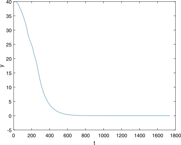
Next, we take some numerical simulations to validate our main results. We set the basic parameters as follows [48]: $d=0.2$, $\beta =0.000024$, $\alpha =0.000024$, $\rho =0.2$, $a=0.15$, $k=150$, $u=0.2$. Firstly, we set $\pi =2$, direct calculations with Maple 14 show that $\mathcal{R}=0.514971<1$ and $E_0=(10,0,0)$. By Theorem 3.1 the virus-free equilibrium $E_0$ of the system is stable (see Figs. 1–4). Next, we change π to 10, direct calculations show that $\mathcal{R}=2.574857>1$, then system (4) has two equilibria, i.e., the virus-free equilibrium $E_0=(50,0,0)$ and the virus equilibrium $E^{\ast }=(19.4186,40.7753,30581.4470)$. It is easy to see that

$$\begin{array}{c}{b}_0=0.0140,\hfill \\ c_0=0.008048,\hfill \\ G(0)=d_0=b_0^2-c_0^2=0.000131>0,\hfill \\ \mathrm{\Delta }=0.148921>0,\hfill \\ z_1^{\ast }=0.240948,\hfill \\ G\left(z_1^{\ast }\right)=-0.008284<0,\hfill \end{array}$$

then equation (12) has two positive roots $z_1=0.0089$ and $z_2=0.3680$, and equation (11) has two positive roots ${\varpi }_1=0.09441603258$ and ${\varpi }_2=0.6066529567$. Therefore we have the Hopf bifurcation value ${\tau }_2^0=3.828340005$.

Figure 2.

Time series for $y(t)$ with the initial value $(19,40,30581)$, where $\mathcal{R}=0.514971<1$

Figure 3.

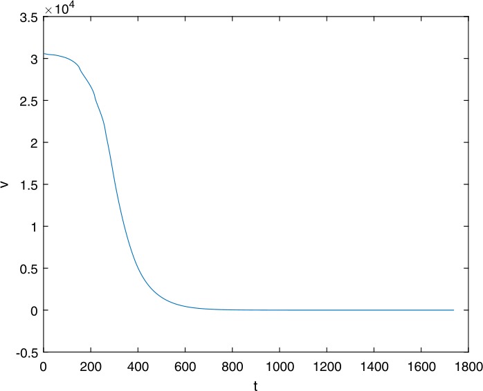
Time series for $v(t)$ with the initial value $(19,40,30581)$, where $\mathcal{R}=0.514971<1$

Figure 1.

Time series for $x(t)$ with the initial value $(19,40,30581)$, where $\mathcal{R}=0.514971<1$

Figure 4.

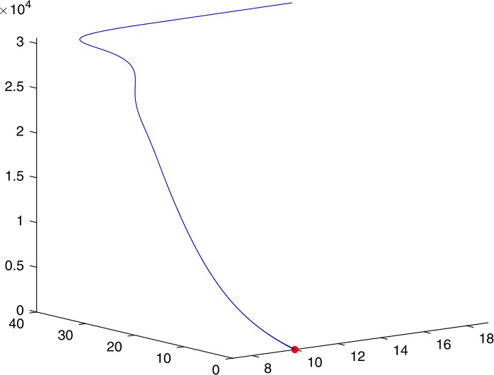
3D phase for $x(t)$, $y(t)$, and $v(t)$ with the initial value $(19,40,30581)$, where $\mathcal{R}=0.514971<1$

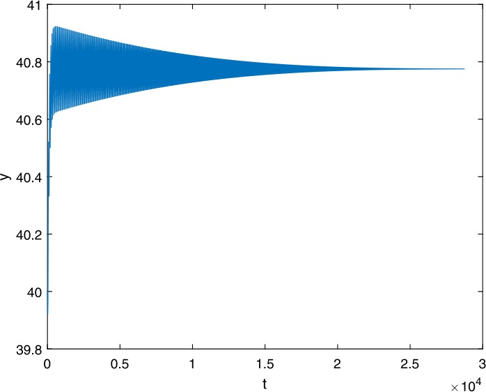
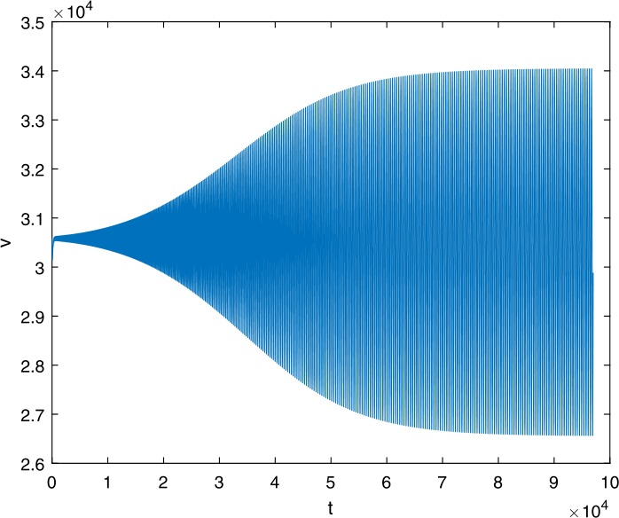
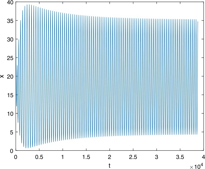
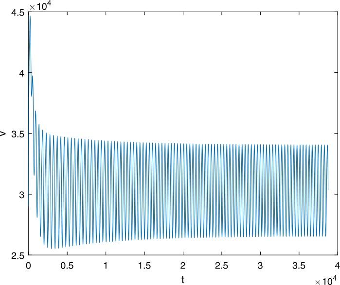
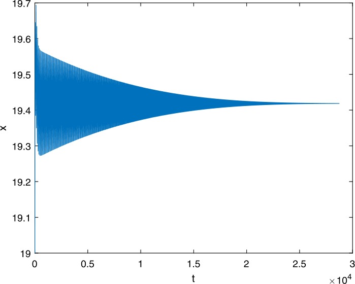
If we set $\tau =3.8<3.828340005$, by Theorem 3.2, the virus equilibrium $E^{\ast }$ is asymptotically stable (see Figs. 5–8). If we set $\tau =3.9>3.828340005$, by Theorem 3.2, the virus equilibrium $E^{\ast }$ is unstable and periodic oscillations occur (see Figs. 9–16 with different initial values).

Figure 6.

Time series for $y(t)$ with the initial value $(19,40,30581)$, where $\mathcal{R}=2.574857>1$

Figure 7.

Time series for $v(t)$ with the initial value $(19,40,30581)$, where $\mathcal{R}=2.574857>1$

Figure 10.

Time series for $y(t)$ with the initial value $(19,40,30581)$, where $\mathcal{R}=2.574857>1$, $\tau =3.8<{\tau }_2^0$

Figure 11.

Time series for $v(t)$ with the initial value $(19,40,30581)$, where $\mathcal{R}=2.574857>1$, $\tau =3.8<{\tau }_2^0$

Figure 12.

3D phase for $x(t)$, $y(t)$, and $v(t)$ with the initial value $(19,40,30581)$, where $\mathcal{R}=2.574857>1$, $\tau =3.8<{\tau }_2^0$

Figure 13.

Time series for $x(t)$ with the initial value $(30,75,29000)$, where $\mathcal{R}=2.574857>1$, $\tau =3.9>{\tau }_2^0$

Figure 14.

Time series for $y(t)$ with the initial value $(30,75,29000)$, where $\mathcal{R}=2.574857>1$, $\tau =3.9>{\tau }_2^0$

Figure 15.

Time series for $v(t)$ with the initial value $(30,75,29000)$, where $\mathcal{R}=2.574857>1$, $\tau =3.9>{\tau }_2^0$

Figure 5.

Time series for $x(t)$ with the initial value $(19,40,30581)$, where $\mathcal{R}=2.574857>1$

Figure 8.

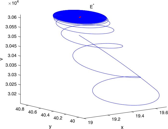
3D phase for $x(t)$, $y(t)$, and $v(t)$ with the initial value $(19,40,30581)$, where $\mathcal{R}=2.574857>1$

Figure 9.

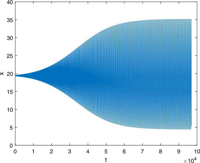
Time series for $x(t)$ with the initial value $(19,40,30581)$, where $\mathcal{R}=2.574857>1$, $\tau =3.8<{\tau }_2^0$

Figure 16.

3D phase for $x(t)$, $y(t)$, and $v(t)$ with the initial value $(30,75,29000)$, where $\mathcal{R}=2.574857>1$, $\tau =3.9>{\tau }_2^0$

Authors’ contributions

All authors read and approved the final manuscript.

Funding

Z.C. Jiang was supported by the National Natural Science Foundation of China (Nos. 11801014 and 11875001), the Natural Science Foundation of Hebei Province (No. A2018409004), Hebei province university discipline top talent selection and training program (SLRC2019020), and Talent Training Project of Hebei Province.

Competing interests

The authors declare that there is no conflict of interests regarding the publication of this paper.

References

- 1.Zhang T., Meng X., Zhang T. Global dynamics of a virus dynamical model with cell-to-cell transmission and cure rate. Comput. Math. Methods Med. 2015;2015:758362. doi: 10.1155/2015/758362. [DOI] [PMC free article] [PubMed] [Google Scholar]
- 2. WHO: World health organization report: research for universal health coverage. Technical report, World Health Organization, (2013). http://www.who.int/whr/en/
- 3.Zhang W., Meng X., Dong Y. Periodic solution and ergodic stationary distribution of stochastic SIRI epidemic systems with nonlinear perturbations. J. Syst. Sci. Complex. 2019;32(4):1104–1124. doi: 10.1007/s11424-018-7348-9. [DOI] [Google Scholar]
- 4. Division of STD Prevention: Prevention of Genital HPV Infection and Sequelae: Report of an External Consultants’ Meeting. Department of Health and Human Services, Atlanta: Centers for Disease Control (1999)
- 5.Winer R.L., Hughes J.P., Feng Q., O’Reilly S., Kiviat N.B., Holmes K.K., Koutsky L.A. Condom use and the risk of genital human papillomavirus infection in young women. N. Engl. J. Med. 2006;354(25):2645–2654. doi: 10.1056/NEJMoa053284. [DOI] [PubMed] [Google Scholar]
- 6.Daling J.R., Madeleine M.M., Johnson L.G., Schwartz S.M., Shera K.A., Wurscher M.A., Carter J.J., Porter P.L., Galloway D.A., Mcdougall J.K. Human papillomavirus, smoking, and sexual practices in the etiology of anal cancer. Cancer. 2004;101(2):270–280. doi: 10.1002/cncr.20365. [DOI] [PubMed] [Google Scholar]
- 7.Parkin M., Bray F. The burden of HPV-related cancers. Vaccine. 2006;24:11–25. doi: 10.1016/j.vaccine.2006.05.111. [DOI] [PubMed] [Google Scholar]
- 8.Chaturvedi A.K., Engels E.A., Pfeiffer R.M., Hernandez B.Y., Xiao W., Kim E., Jiang B., Goodman M.T., Sibugsaber M., Cozen W. Human papillomavirus and rising oropharyngeal cancer incidence in the United States. J. Clin. Oncol. 2011;29(32):4294–4301. doi: 10.1200/JCO.2011.36.4596. [DOI] [PMC free article] [PubMed] [Google Scholar]
- 9.Cui J., Zhang Y., Feng Z., Guo S., Zhang Y. Influence of asymptomatic infections for the effectiveness of facemasks during pandemic influenza. Math. Biosci. Eng. 2019;16(5):3936–3946. doi: 10.3934/mbe.2019194. [DOI] [PubMed] [Google Scholar]
- 10.Feng T., Qiu Z. Global analysis of a stochastic TB model with vaccination and treatment. Discrete Contin. Dyn. Syst., Ser. B. 2019;24(6):2923–2939. [Google Scholar]
- 11.Zhao W., Liu J., Chi M., Bian F. Dynamics analysis of stochastic epidemic models with standard incidence. Adv. Differ. Equ. 2019;2019(1):22. doi: 10.1186/s13662-019-1972-0. [DOI] [Google Scholar]
- 12.Feng T., Qiu Z., Meng X. Analysis of a stochastic recovery-relapse epidemic model with periodic parameters and media coverage. J. Appl. Anal. Comput. 2019;9(3):1007–1021. [Google Scholar]
- 13.Zhou X., Song X., Shi X. A differential equation model of HIV infection of CD4+ T-cells with cure rate. J. Math. Anal. Appl. 2008;342(2):1342–1355. doi: 10.1016/j.jmaa.2008.01.008. [DOI] [Google Scholar]
- 14.Li J., Song X., Gao F. Global stability of a viral infection model with two delays and two types of target cells. J. Appl. Anal. Comput. 2012;2(3):281–292. [Google Scholar]
- 15.Xu R. Global stability of an HIV-1 infection model with saturation infection and intracellular delay. J. Math. Anal. Appl. 2011;375(1):75–81. doi: 10.1016/j.jmaa.2010.08.055. [DOI] [Google Scholar]
- 16.Shu H., Wang L. Role of cd4+ t-cell proliferation in HIV infection under antiretroviral therapy. J. Math. Anal. Appl. 2012;394(2):529–544. doi: 10.1016/j.jmaa.2012.05.027. [DOI] [Google Scholar]
- 17.Guidotti L.G., Rochford R., Chung J., Shapiro M., Purcell R., Chisari F.V. Viral clearance without destruction of infected cells during acute HBV infection. Science. 1999;284(5415):825–829. doi: 10.1126/science.284.5415.825. [DOI] [PubMed] [Google Scholar]
- 18.Wang K., Fan A., Torres A. Global properties of an improved hepatitis B virus model. Nonlinear Anal., Real World Appl. 2010;11(4):3131–3138. doi: 10.1016/j.nonrwa.2009.11.008. [DOI] [Google Scholar]
- 19.Dahari H., Shudo E., Ribeiro R.M., Perelson A.S. Modeling complex decay profiles of hepatitis B virus during antiviral therapy. Hepatology. 2009;49(1):32–38. doi: 10.1002/hep.22586. [DOI] [PMC free article] [PubMed] [Google Scholar]
- 20.Qian H., Ning P., Wei D. Global stability for a dynamic model of hepatitis B with antivirus treatment. J. Appl. Anal. Comput. 2013;3(1):37–50. [Google Scholar]
- 21.Feng T., Qiu Z., Meng X., Rong L. Analysis of a stochastic HIV-1 infection model with degenerate diffusion. Appl. Math. Comput. 2019;348:437–455. [Google Scholar]
- 22.Cui J., Ying C., Guo S., Zhang Y., Sun L., Zhang M., He J., Song T. Influence of media intervention on AIDS transmission in MSM groups. Math. Biosci. Eng. 2019;16(5):4594–4606. doi: 10.3934/mbe.2019230. [DOI] [PubMed] [Google Scholar]
- 23.Ji Y., Ma W., Song K. Modeling inhibitory effect on the growth of uninfected T cells caused by infected T cells: stability and Hopf bifurcation. Comput. Math. Methods Med. 2018;2018:3176893. doi: 10.1155/2018/3176893. [DOI] [PMC free article] [PubMed] [Google Scholar]
- 24.Guo S., Ma W. Global behavior of delay differential equations model of HIV infection with apoptosis. Discrete Contin. Dyn. Syst., Ser. B. 2016;21(1):103–119. doi: 10.3934/dcdsb.2016.21.103. [DOI] [Google Scholar]
- 25.Song Y., Miao A., Zhang T., Wang X., Liu J. Extinction and persistence of a stochastic SIRS epidemic model with saturated incidence rate and transfer from infectious to susceptible. Adv. Differ. Equ. 2018;2018(1):293. doi: 10.1186/s13662-018-1759-8. [DOI] [Google Scholar]
- 26.Gao N., Song Y., Wang X., Liu J. Dynamics of a stochastic SIS epidemic model with nonlinear incidence rates. Adv. Differ. Equ. 2019;2019(1):41. doi: 10.1186/s13662-019-1980-0. [DOI] [Google Scholar]
- 27.Miao A., Zhang T., Zhang J., Wang C. Dynamics of a stochastic SIR model with both horizontal and vertical transmission. J. Appl. Anal. Comput. 2018;8(4):1108–1121. [Google Scholar]
- 28.Fan X., Song Y., Zhao W. Modeling cell-to-cell spread of HIV-1 with nonlocal infection. Complexity. 2018;2018:2139290. [Google Scholar]
- 29.Perelson A.S., Nelson P.W. Mathematical analysis of HIV-1 dynamics in vivo. SIAM Rev. 1999;41(1):3–44. doi: 10.1137/S0036144598335107. [DOI] [Google Scholar]
- 30.Perelson A.S., Neumann A.U., Markowitz M., Leonard J.M., Ho D.D. HIV-1 dynamics in vivo: virion clearance rate, infected cell life-span, and viral generation time. Science. 1996;271(5255):1582–1586. doi: 10.1126/science.271.5255.1582. [DOI] [PubMed] [Google Scholar]
- 31.Nelson P.W., Perelson A.S. Mathematical analysis of delay differential equation models of HIV-1 infection. Math. Biosci. 2002;179(1):73–94. doi: 10.1016/S0025-5564(02)00099-8. [DOI] [PubMed] [Google Scholar]
- 32.Mcdonald D., Hope T.J. Recruitment of HIV and its receptors to dendritic cell–T cell junctions. Science. 2003;300(5623):1295–1297. doi: 10.1126/science.1084238. [DOI] [PubMed] [Google Scholar]
- 33.Sattentau Q. Avoiding the void: cell–to–cell spread of human viruses. Nat. Rev. Microbiol. 2008;6(11):815–826. doi: 10.1038/nrmicro1972. [DOI] [PubMed] [Google Scholar]
- 34.Phillips D.M. The role of cell–to–cell transmission in HIV infection. AIDS. 1994;8(6):719–732. doi: 10.1097/00002030-199406000-00001. [DOI] [PubMed] [Google Scholar]
- 35.Sato H., Orensteint J., Dimitrov D., Martin M. Cell-to-cell spread of HIV-1 occurs within minutes and may not involve the participation of virus particles. Virology. 1992;186(2):712–724. doi: 10.1016/0042-6822(92)90038-Q. [DOI] [PubMed] [Google Scholar]
- 36.Jolly C. Cell–to–cell transmission of retroviruses: innate immunity and interferon-induced restriction factors. Virology. 2011;411(2):251–259. doi: 10.1016/j.virol.2010.12.031. [DOI] [PMC free article] [PubMed] [Google Scholar]
- 37.Bangham C.R. The immune control and cell–to–cell spread of human T–lymphotropic virus type 1. J. Gen. Virol. 2003;84(12):3177–3189. doi: 10.1099/vir.0.19334-0. [DOI] [PubMed] [Google Scholar]
- 38.Krantic S., Gimenez C., Rabourdincombe C. Cell–to–cell contact via measles virus haemagglutinin-CD46 interaction triggers CD46 downregulation. J. Gen. Virol. 1995;76(11):2793–2800. doi: 10.1099/0022-1317-76-11-2793. [DOI] [PubMed] [Google Scholar]
- 39.Wild T.F., Malvoisin E., Buckland R. Measles virus: both the haemagglutinin and fusion glycoproteins are required for fusion. J. Gen. Virol. 1991;72(2):439–442. doi: 10.1099/0022-1317-72-2-439. [DOI] [PubMed] [Google Scholar]
- 40.Spouge J.L., Shrager R.I., Dimitrov D.S. HIV-1 infection kinetics in tissue cultures. Math. Biosci. 1996;138(1):1–22. doi: 10.1016/S0025-5564(96)00064-8. [DOI] [PubMed] [Google Scholar]
- 41.Herz A.V., Bonhoeffer S., Anderson R.M., May R.M., Nowak M.A. Viral dynamics in vivo: limitations on estimates of intracellular delay and virus decay. Proc. Natl. Acad. Sci. 1996;93(14):7247–7251. doi: 10.1073/pnas.93.14.7247. [DOI] [PMC free article] [PubMed] [Google Scholar]
- 42.Culshaw R.V., Ruan S., Webb G. A mathematical model of cell-to-cell spread of HIV-1 that includes a time delay. J. Math. Biol. 2003;46(5):425–444. doi: 10.1007/s00285-002-0191-5. [DOI] [PubMed] [Google Scholar]
- 43.Lai X., Zou X. Modeling cell-to-cell spread of HIV-1 with logistic target cell growth. J. Math. Anal. Appl. 2015;426(1):563–584. doi: 10.1016/j.jmaa.2014.10.086. [DOI] [Google Scholar]
- 44.Routh E.J., Clifford W.K., Sturm C., Bocher M. Stability of Motion. London: Taylor & Francis; 1975. [Google Scholar]
- 45.Ruan S., Wei J. On the zeros of a third degree exponential polynomial with applications to a delayed model for the control of testosterone secretion. IMA J. Math. Appl. Med. Biol. 2001;18(1):41. doi: 10.1093/imammb/18.1.41. [DOI] [PubMed] [Google Scholar]
- 46.Hassard B.D., Kazarinoff N.D., Wan Y.H. Theory and Applications of Hopf Bifurcation. Cambridge: Cambridge University Press; 1981. [Google Scholar]
- 47.Hale J., Lunel M. Introduction to Functional Differential Equations. New York: Springer; 1993. [Google Scholar]
- 48.Zhuang K., Zhu H. Stability and bifurcation analysis for an improved HIV model with time delay and cure rate. WSEAS Trans. Math. 2013;12(8):860–869. [Google Scholar]