Abstract
Many of the structural characteristics of a network depend on the connectivity with and within the hubs. These dependencies can be related to the degree of a node and the number of links that a node shares with nodes of higher degree. In here we revise and present new results showing how to construct network ensembles which give a good approximation to the degree–degree correlations, and hence to the projections of this correlation like the assortativity coefficient or the average neighbours degree. We present a new bound for the structural cut–off degree based on the connectivity within the hubs. Also we show that the connections with and within the hubs can be used to define different networks cores. Two of these cores are related to the spectral properties and walks of length one and two which contain at least on hub node, and they are related to the eigenvector centrality. We introduce a new centrality measured based on the connectivity with the hubs. In addition, as the ensembles and cores are related by the connectivity of the hubs, we show several examples how changes in the hubs linkage effects the degree–degree correlations and core properties.
Subject terms: Computational science, Information technology
Introduction
What does the Internet, the human brain connectome and the super–heroes have in common? If the connectivity of the Internet, the brain and the friendship between the super–heroes is represented with a network, there exist a small set of nodes which have a large numbers of links, the so–called rich nodes, hubs or stars1–3. Rich nodes can or cannot have connections between themselves. If they do, we can interpret this as the presence of a core, a set of well connected nodes that are well connected between themselves.
The connectivity within rich nodes has been associated with many structural characteristics of a network like assortativity4, clustering coefficient4, existence of motifs5, the stability of dynamical processes6 and the construction of network’s null–models7. The aim here is to bring together previous and new results by showing the dependance of these network properties with the node’s degree and the number of links that a node shares with nodes of higher degree.
The first step to describe a network is via its degree sequence {ki}, i = 1, …, N, which it is used to measure the network’s degree distribution P(k), that is, the fraction of nodes with degree k.
A better description can be obtained from the degree–degree correlation , the probability that an arbitrary link connects a node of degree k with a node of degree . In scale–free networks it is not possible from network’s measurements to evaluate accurately the degree–degree correlation due to the small number of nodes with high degree and the finite size of the network, hence, the structure of the network is characterised using different projections of the degree–degree correlation, like the assortativity coefficient ρ8 or the average degree of the nearest neighbours ⟨knn(k)⟩9. Here we show that it is possible to obtain a good approximation to the degree–degree correlation, even for power law networks, via the connectivity within the hubs.
The relationship between the degree–degree correlation and the network hubs is based on the observation that the links between the well connected nodes have a strong effect on the network’s assortativity, and also, it has been observed that the assortativity influences properties like the diffusion of information or the clustering coefficient. These observations motivates the question: if the hubs have such a large effect in some of the network properties, which of these hubs form the core of a network? Here we consider cores that are defined via the shared number of links within the hubs.
The definition of the cores considered here differs from the core–periphery introduced by Borgatti and Everett10, where the core is a set of nodes that are densely interconnected and share some connections with the periphery nodes. Here we do not impose any restriction on the poorly connected nodes, the periphery.
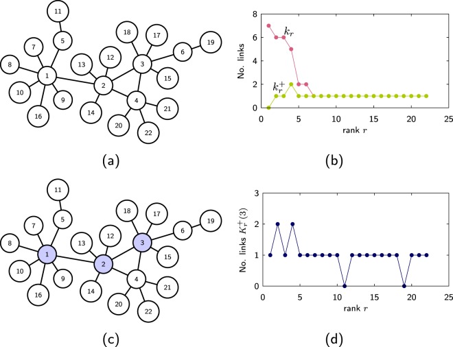
In an undirected network the connectivity of its nodes is described by their degree k. Two of the simplest properties of a network are its maximum degree , i = 1, …, N and its average degree /N = 2L/N, where N is the total number of nodes and L is the total number of links. The degree sequence {ki} gives only partial information about the network structure, a better description can be obtained from the number of links that a node shares with nodes of higher degree. Here, we assume that the sequence {ki} contains the node’s degree ranked in decreasing order, that is, node 1 has the largest degree k1, node 2 the second largest degree k2 and so on. The sequence describes the number of links that node i has with the i −1 nodes of higher rank (see Fig. 1(a,b)). The term is bounded by the degree and satisfies that . For networks where multilinks are not allowed, satisfies the bound , that is, the node of rank i cannot have more than i −1 links with the i −1 nodes of larger rank.
Figure 1.
(a) A network where its nodes are ranked in decreasing order of their degree and (b) the degree kr of node r and the number of links that node r has with nodes of higher rank. (c) The same network where the three top ranked nodes form a core and (d) number of links that node r has with the any of these three top ranked nodes.
The other sequence considered here is defined by first taking a subset of the top r ranked nodes, then describes the number of links that node i has with this set (see Fig. 1(c,d)). The sequence gives information about the “influence” that the top r nodes have on the network. The sequences {ki}, and can be extended to weighted networks. If the nodes are ranked in decreasing order of their weight wi, then would be the total weight that node i shares with nodes of greater rank and would be the total weight that node i shares with the top r nodes.
In here we revise and extend some previous results showing that from the sequences {ki} and it is possible to build network ensembles where the degree–degree correlation is well defined from the data. We introduce a new structural cut–off degree in the case that the ensemble describes the average connectivity of the networks. We present several examples to show the association between the connectivity of the hubs and assortativitiy and clustering coefficients.
Also we revise some previous results showing how the sequences {ki}, and can be used to define different cores of the network, including the rich–club. We show that some cores based on the connectivity of the well connected are closely related to the eigenvector centrality and how can be used to define a network’s core and a new centrality measure based on a core–biased random walker. The section ends with comments about the communicability11 and the time evolution of the cores. The Methods sections contains the derivations of the results and Supplementary information.
Results
Ensembles and correlations
The approach is to create different sets of ensembles which are defined via the sequences {ki} and then show that, from these ensembles, it is possible to obtain a good approximation to the degree–degree correlation. The motivation behind this approach is that a network with positive assortativity coefficient has the property that nodes of high degree tend to connect to nodes of high degree, this property would be reflected in the sequence as it is expected that the well connected nodes share connections with other well connected nodes. Hence a network ensemble constructed from the sequences {ki} and of a given network would have a similar degree–degree correlation as the given network.
Maximal entropy approach
The information contained in {ki} and can be used to construct a network ensemble via Shannon’s entropy12–18. The Shannon entropy for a network is where pij is the probability that i shares links with node j. The maximisation of this entropy is attractive because it produces null-models with probabilistic characteristics only warranted by the data. The ensemble obtained from the maximisation of the entropy satisfy the soft constraints and , where the total number of links L is conserved and no self–loops are allowed, i.e. prr = 0. The maximal entropy solution under these constraints is given by the probabilities7
| 1 |
where
| 2 |
The values of s(m) are defined recursively with the initial condition s(1) = 1. As we are considering undirected networks pij = pji. The average number of links between nodes i and j is eij = Lpij with variance var(eij) = Lpij(1 −pij). This maximal entropy solution can be used to construct the following ensembles:
If the sequences {ki} and are conserved, the networks from the ensemble have similar correlations as the original network. This ensemble has been studied before7 but here we extend it as follows.
If the sequence {ki} is given but the sequence is defined up to the constraint , then the ensemble would have the same degree sequence and on average two nodes would have only one link.
If in the ME2 ensemble we remove the restriction , then the ensemble would have the same degree sequence but it is possible to have, on average, more than one link per pair of nodes.
These ensembles produce networks with different statistical properties which can be measured via the average neighbour degree or the assortativity coefficient. The first ensemble consist of networks with similar correlation than the data. The second ensemble consist of networks where the correlation is zero if the maximal degree is smaller than the structural cut–off degree . If the the maximal degree is greater than cut–off degree then the network is correlated due to structural constraints9 and it is not possible to construct an uncorrelated network without introducing multiple links between nodes. The third ensemble produces uncorrelated networks if multiple links between nodes are allowed. From the Kullback–Leibler divergence we observed that the amount of information to describe the ensembles decreases as the restrictions on the sequence {k+} is relaxed, that is ME3 contains more information than ME2 which contains more information than ME1 (see Methods). It is not difficult to generate a network that is a member of one of the previous ensembles, the network is generated using a Bernoulli process where the existence of a link between nodes i and j is given by pij.
The average nearest neighbours degree given by , where is the conditional probability that given a node with degree k its neighbour has degree . For an uncorrelated network /⟨k⟩. In our case7
| 3 |
where if ki = k and zero otherwise. The assortativity coefficient is given by
| 4 |
where ⟨…⟩ℓ is the average over all links.
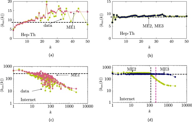
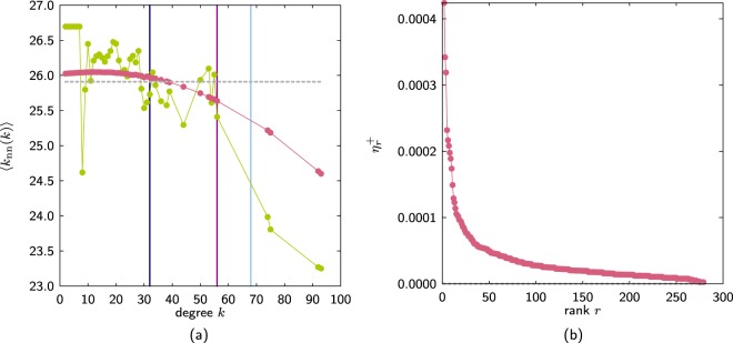
As an example, Fig. 2 show the average neighbours degree for the Hep-Th network and the AS-Internet network. For both networks the ME1 method produces ensembles with similar correlations as the original network (see Fig. 2(a,c)). For the Hep–Th network its maximal degree is less than the cut–off degree so it is expected that the maximal entropy networks produced by the ME2 and ME3 methods generate uncorrelated networks (Fig. 2(b)). For the AS–Internet the maximal degree is greater than the structural cut–off degree kcut, in this case the ME2 produce ensembles where only the links with end nodes of degree lower than kcut are uncorrelated (Fig. 2(d)). For the ME3 ensemble, multilinks are allowed, and the correlation shown in the figure is due to the structural constraint that self–loops are no allowed.
Figure 2.
(a) Average neighbours degree (green line) for the Hep-Th network and the ensemble ME1 (pink line). (b) For the Hep-Th the ensembles obtained by the ME2 (green line) and ME3 (dark blue line) methods produce uncorrelated networks. (c) Average neighbours degree (green line) for the AS-Internet network and the ensemble obtained using the ME1 (pink line) method showing that ME1 approximates well . (d) For the AS-Internet the ME2 (green line) and ME3 (dark blue line) produce ensembles that show correlations for the links that include nodes of high degree. The orange dotted line marks the value of the cut-off degree . The grey dotted vertical line shows the structural cut–off degree obtained from Eq. (6). The dashed horizontal line shows the value ⟨knn(k)⟩ = ⟨k2⟩/⟨k⟩ for the uncorrelated network.
In the case of weighted networks, Eqs. (1)-(2) are still valid. In this case the links have weights wi and the network is described by the sequences {wi} and instead of {ki} and . For the ME3 ensemble the probabilities pij are well approximated via the configuration model pij = (wiwj)/L2, and is well approximated via
| 5 |
From this equation we derived a new structural cut–off degree for unweighted networks. If we consider that is approximated via and in networks where multilinks are not allowed then the condition for a multilink is
| 6 |
The structural cut–off degree corresponds to the node with the largest rank i where the above condition is true (see Fig. 2(d)). We can consider this structural cut–off also as a core of the network, these are the nodes that due to the structural constraints introduce correlations between the nodes.
Restricted randomisation
The maximal entropy approach generates (canonical) ensembles with the soft constraints ⟨ki⟩ = ki and . In the case that what it is required is an ensemble where the networks ensembles satisfies hard constraints (micro–canonical), that is that the sequences {ki} and are conserved, the approach is to generate the ensemble numerically using a restricted randomisation approach19. As in the case of the ME1 ensemble, the networks obtained from the restricted randomisation have similar degree–degree correlations as the original network20. For the case that maximal degree is smaller than the structural cut–off degree and only the degree sequence is conserved, the restricted randomisation would generate uncorrelated networks as the ensembles ME2 and ME3, in this case the link probabilities are well approximated by the configuration model. If the maximal degree is larger than the cut–off degree then the networks forming the restricted randomisation ensemble would have different degree–degree correlations than the networks from the ME2 and the ME3 ensembles18,21. Finally it is worth noting these ensembles do not impose the condition that the randomised network should be one connected piece, in the case that this condition is imposed, the correlations describing the ensemble could change as shown recently by Ring et al.22
Clustering and correlations
In networks where the structure can be fully described from the degree distribution and the degree–degree correlation, the expected number of triangles and hence the clustering coefficient can be evaluated from the ensemble23.
Figure 3(a,b)show the number of triangles Ti that node i has with nodes j and k which are of higher rank, i > j > k and the average number of triangles ⟨Ti⟩ obtained from the ME1 ensemble. Notice that for this ensemble, due to the soft constraints, it is possible to have more than one link between two nodes and this could have a large effect on the number of triangles. Figure 3(a) shows the results for the AS–Internet where the approximation Ti via ⟨Ti⟩ is good because the structure of the 1997 AS–Internet can be described with the degree distribution and the degree–degree correlation1,24,25. Figure 3(b) shows the case for the Hep–Th network. In this case the number of triangles of the network differs considerably from the ME1 ensemble because to fully describe the structure of this network we need higher order correlations. However, even that ⟨Ti⟩ can be orders of magnitude less than Ti, the trend between these two quantities is similar, verifying that the degree correlations strongly affect the frequency of triangles25.
Figure 3.
Number of triangles Tr (green line) and its approximation using the ME1 ensemble (pink line) (a) for the AS–Internet and (b) for the Hep–Th.
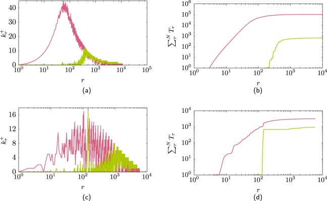
The connectivity within the hubs has a significant impact in the number of triangles in a network. Figure 4(a) shows for two networks. Both networks have the same degree distribution as the AS–Internet but one network has the maximal possible connectivity within the hubs (pink) and the other network has the minimal possible connectivity within the hubs (green). The networks were created using restricted randomisation so there are no multilinks. Figure 4(b) shows the cumulative number of triangles for these networks as the rank increases. Notice that the difference is almost two orders of magnitude between the network with maximal hub connectivity against the one with minimal hub connectivity. However both networks have similar assortativity coefficient due to the structural correlations as for both of these networks .
Figure 4.
(a) Difference in the hub connectivity for two networks that have the same degree distribution as the AS-Internet. One network has maximal connectivity within the nodes (pink line) (ρ = −0.181) and the other minimal connectivity within the hub nodes (green line) (ρ = −0.20). (b) This change of connectivity is reflected in the number of triangles in each network, where the network with maximal hub connectivity (pink line) has almost two orders of magnitude more triangles that the other network (green line). (c,d) Similar as (a,b) but for the Hep–Th network where assortativity coefficients ρ = 0.69 and ρ = −0.42.
Figure 4(c,d)show the case of two networks which have the same degree distribution as the Hep–Th. Again the difference between the networks is the connectivity within the hubs, and again as in the previous case, decreasing the connectivity of the hubs decreases the number of triangles in the network. In this case there are no structural constraints and the two networks have very different assortativity coefficient. The network with maximal connectivity of the hubs is assortative (ρ = 0.69) compare with the other network which is dis-assortative (ρ = −0.42). This is an example where the change on the connectivity of the hubs has a drastic effect on the assortativity coefficient and the number of triangles in the network.
Cores
The degree sequence gives a centrality measure to distinguish the nodes. It is common to assume that nodes of higher degree are more important and form the core of the network. There are several possibilities to define a core via the sequences and .
The rich–core
One of the simplest ways to define a core is via the rich–core26. The core is a set of well connected nodes, that is the top rc ranked nodes. The boundary of the rich–core is the rank rc where is maximal. The core are all the nodes with rank less than rc.
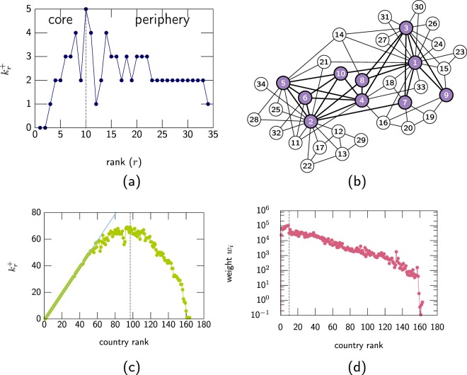
Figure 5(a) show an example of this core for the Karate club. The maximum value happens at rc = 10 so the top 10 nodes form the core, the core is shown in Fig. 5(b). The partition of a network via the properties of is attractive due to its simplicity and this partition has been used to define the core of the C. elegans and its time evolution26, in the characterisation of food webs27 and recently in the concept of rich–core has been extended to multiplexes when studying the brain connectivity28.
Figure 5.
(a) Rich–core for the Karate network defined by the maximum of at r = 10. The members of the core are the top 10 ranked nodes as shown in (b). (c) Example of of the trade relationship between WTO countries in 1980. The core of this network is the top 97 ranked nodes (dash vertical line). The diagonal line (light blue) shows the value where the top ranked nodes form a clique. (d) The weighted w+ for the WTO countries where w+ is related to the trade in dollars. The core is the top ten ranked nodes (dash vertical line). Notice that the vertical axis is in logarithmic scale.
The rich–core can also be evaluated in weighted networks. Figure 5(c,d) show the rich–core of two networks describing the trade between nations in 1980 as reported by the World Trade Organisation (WTO). In Fig. 5(c) shows which in this case corresponds to the number of trade relationships that country r has with countries that have at least the same amount of trade relationships as country r. The figure also shows the line r −1, this line is the maximum amount of trade relationships that country r can have with countries of higher rank. It is clear that the top 50 countries form an almost fully connected clique. The core is formed by 97 countries which is almost 60% of total number of countries reported in the WTO dataset for 1980. Figure 5(d) shows , the trade relationship weighted by the amount of dollars (exporting goods) that country r has with countries that are larger exporters in value than itself. In this case the core is formed by only 10 countries, that is around 6% of the countries. The cores defined by and show two different views of the trade between nations. There is a large number of trade agreements between nations and a large number of nations are part of the core of these agreements, however by value less than 10 nations form the core.
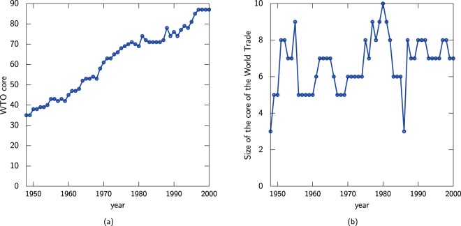
The evolution of the hubs can be described via the rich–core. Figure 6(a,b) shows the evolution of the cores from 1950–2000 for the trade relationships and weighted relationships between countries. The amount of trading nations has increased from 1950–2000 (Fig. 6(a)), perhaps due to globalisation and the core of trading nations has become larger with time. However by wealth (Fig. 6(b)), the size of the core has not changed much, less than ten countries dominate the market by value.
Figure 6.
Evolution of the rich–core by (a) trade relationships between countries and (b) by value of exports between countries.
The spectral–core
Another common measure of centrality is the eigenvector–centrality. In this case a node is important if it is connected to other important nodes. It is know that in many networks the degree centrality of a node is correlated to its eigenvector centrality so it is natural to ask what is the contribution of the nodes with high degree centrality to their eigenvector centrality.
For an undirected and unweighted network whose connectivity is described by the adjacency matrix A, the spectrum of the network is the set of eigenvalues Λ1 ≥ Λ2… ≥ ΛN of A. The highest eigenvalue Λ1 plays an important role when describing information diffusion or epidemic transmission on a network29–32.
It is known that the spectral radius Λ1 increases with the assortativity coefficient and it is related to the number of triangles in the networks33–35, so it is expected that changes in the hubs connectivity would also change the spectral radius. For the eigenvalue Λ1, its corresponding eigenvector is the eigenvector centrality where the entry is the “importance” of node i.
The sequence can be used to define a lower bound for Λ136
| 7 |
where the is the average number of links shared by the top r nodes. This bound can be used to define a core. The spectral–core boundary is the rank rc where is maximal. This correspond to the best bound of Λ1 based on . Similarly as the rich–core, any node with rank less than rc belong to the core.
This bound can also be used to create an approximation of the eigenvector centrality . If the core is defined by the rank rc then an approximation to is the vector with entries where is the number of links that node i shares with the top rc nodes.
The bound of Λ1 can be improved if we consider the average of links which have at least one of its end nodes in the core
| 8 |
which is the average number of links that connect to the top r nodes. The core boundary is defined by the value of r when h(r) is maximal. The bound in this case is . It is also possible to construct an approximation to the eigenvector centrality from this bound. If W2(rc, i) are the number of walks of length two that start in one of the rc top nodes and end up in any other node i then the approximation to the eigencentrality has entries yi = W2(rc, i). Interestingly in this approximation we not only consider the nodes that form the core but also nodes that connect directly to the core.
As an example we show the spectral core for the EU–Air transportation networks. The dataset consist of the 37 airlines that connect 450 different European airports. First we consider a simple version of this network. The nodes represent different EU airports and a links represent if there is a connection between two airports via a flight. We do not consider the number of flights between two airports or differentiate the airlines.
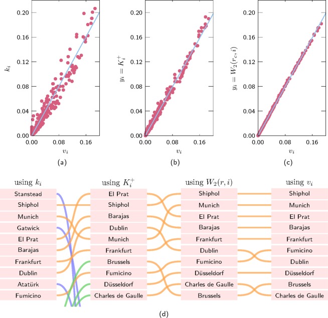
Figure 7 shows the approximation of the eigencentrality via the degree of the nodes (Fig. 7(a)), the number of links connecting to the core (Fig. 7(b)) and the number of walks of length one that finish in the core yi = W2(rc, i) (Fig. 7(c)). The size of the spectral–core is 82 nodes. The spectral core based on the walks of length two gives a good approximation to the eigencentrality. Figure 7(d) shows the airports ranked in decreasing order of the different centralities.
Figure 7.
Correlation between the eigencentrality and its approximations for the EU Air transportation network. (a) Approximation using the degree, (b) and (c) yi = W2(rc, i). (d) Change on the ranking of the top nodes when ranked by decreasing order of their degree ki, , yi = W2(rc, i) and the eigencentrality vi.
We finish this section with two observations. The size of the core is not related to the assortativity of the network, it is possible to have networks with small core which are disassortative, e.g. the AS–Internet. The other observation is that in networks that are highly disassortative the approximation to the largest eigenvalue (Eq. (8)) can be good, however this not translates to a good approximation to the eigencentrality (see Methods for an example).
Biased-random walk core and centrality
Random walks on networks are used to understand structural properties of networks like community detection37, centrality of nodes38, discovery of the network structure39 and the partition of a network into core–periphery40. The maximal entropy random walk41 (MERW) has the property that the random walker would visit walks of same length with equal probability. This kind or random walks have been used to study different properties of complex networks42,43 and in some applications44,45.
In the Maximal Entropy Random Walk (MERW) the transition probability from node i to node j is41
| 9 |
where (A)ij is the i, j entry of the adjacency matrix and vi is the i–th entry of the eigenvector centrality . The stationary probability , which is the probability of finding the walker in node i as time tends to infinity, for the MERW is .
If the largest eigenvalue-eigenvector pair is not known an approximation to the the MERW can be obtained from an approximation to the eigenvector . As mentioned in the spectral–core section, , gives an approximation to the eigenvector .
A biased random walk based on this approximation is46
| 10 |
The term 1 in the numerator and denominator is added as it it is possible that if node j has no links with node of rank greater than r and then the random-walk will be ill-defined. This core–biased random walk describes the dynamics of a random–walker which prefers to jump to the hubs that have many connection with other hubs.
The MERW has the property that in networks where hubs are present, the stationary probability of the hubs is relatively large, there is an argument47,48 saying that the property of concentrating the eigencentrality in the hubs is an undesirable property as diminishes the effectiveness of the centrality as a tool for quantifying the importance of nodes.
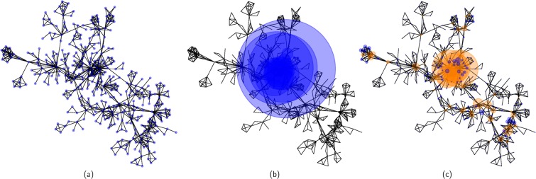
The core–biased random walk is based on the hubs, the relevant hubs are the ones that are well connected with other hubs, this is reflected in the stationary probability which we can consider as a new centrality measure based only in the interconnectivity of the hubs (see Methods for the evaluation of ). Figure 8(a–c) shows the plots of the network-scientist network where Fig. 8(a) shows the layout of the network, Fig. 8(b) shows the same layout but with the radius of the nodes proportional to the eigenvector centrality i.e. . As noticed before the eigencentrality is concentrate in the hub nodes and diminishes the importance of nodes of low degree. Figure 8(c) shows the network with the radius proportional to the stationary probability obtained by the core-biased random walk. In the figure the orange nodes are the core of the network and now nodes of low degree are part of the core as they are locally important.
Figure 8.
(a) Graph of the Network Scientist network. (b) The same graph but the radius of the nodes is proportional to where vi are the entries of the eigencentrality. (c) In this case the radius of the nodes is proportional to the stationary probability of the core–biased random walk. The orange nodes are the core of the network. The core is the top ranked 54 nodes.
The rich–club
The measure which describes how tightly the rich–nodes are interconnected is the rich-club coefficient1. This coefficient is the ratio between the number of connections that the rich–nodes have against the maximum number of connections that they could have, that is the density of connections within the hubs which can be expressed in terms of as
| 11 |
where the sum is the total number of links shared by the top r nodes and the factor (r(r −1))/2 is the total number of links that can exist between these nodes. It is also common to define the rich–club coefficient in terms of the degree49, in this case,
| 12 |
where E>k is the number of links shared between the nodes of degree greater than k and N>k is the number of nodes that have degree greater than k. Notice that the rank based and degree based rich-clubs are related by Φ(r>k) = ϕ(k), where r>k is the node with lowest rank and degree greater than k then and r>k = N>k. The rich–club coefficient and its generalisations have been proved to be a useful measure for studying complex networks49–56. In recent years it has been used to describe the connectivity of the brain, the connectome2,57–62.
Originally the rich–club was defined as the set of nodes that are tightly connected1, that is the set of nodes where the rich–club coefficient is or tends to 1. A clique would have a rich–club coefficient of 1. Colizzaet al.49 introduce an alternative definition. They defined the rich–club as the set of high degree nodes that have a density of connections higher than expected. The expected number of links between the top ranked nodes is evaluated from a random network which is considered as a null model. If ϕrand(k) is the rich-club coefficient of a random network which has the same degree sequence as the original network then the comparison between the network and the null model is done via the normalised rich-club coefficient ϕnorm(k) = ϕ(k)/ϕrand(k). Colizza et al.49 stated that an indicator of a rich-club with respect to the null-model is when the normalised rich-club coefficient is greater than 1. From this definition the normalised rank–based rich–club is
| 13 |
where denotes the connectivity of node i with nodes or larger rank obtained from one of the ensembles or by restricted randomisation. If the maximal degree present in the network is less than the structural cut–off degree then the uncorrelated rich–club can be approximated via (see Methods)
| 14 |
and the normalised rich-club is
| 15 |
Changes related to the core connectivity
The change of connectivity between the hubs could happen due to the disappearance and/or the reshuffling of some of its links, here we consider that some links between hubs are removed. As the cores are defined via the connectivity of the hubs, any change in this connectivity would result in a change of which nodes belong to the core.
The changes in the assortativity coefficient would be constraint if the maximal degree is larger than the cut–off degree, if this is the case, changes in the hubs connectivity would have little effect on the degree–degree correlations. The changes of the hub connectivity have a large impact in the number of triangles and longer loops in the network. Recently, it was suggested57 that a good measure to quantify the changes of the network connectivity is to use the communicability11 of a network.
The communicability between nodes p and q is defined via the weighted sum of all walks between p and q as
| 16 |
where Λp is the p-th eigenvalue and is the j entry of the eigenvector p-th eigenvector. The communicability has the property that it is affected by structural changes of the walks.
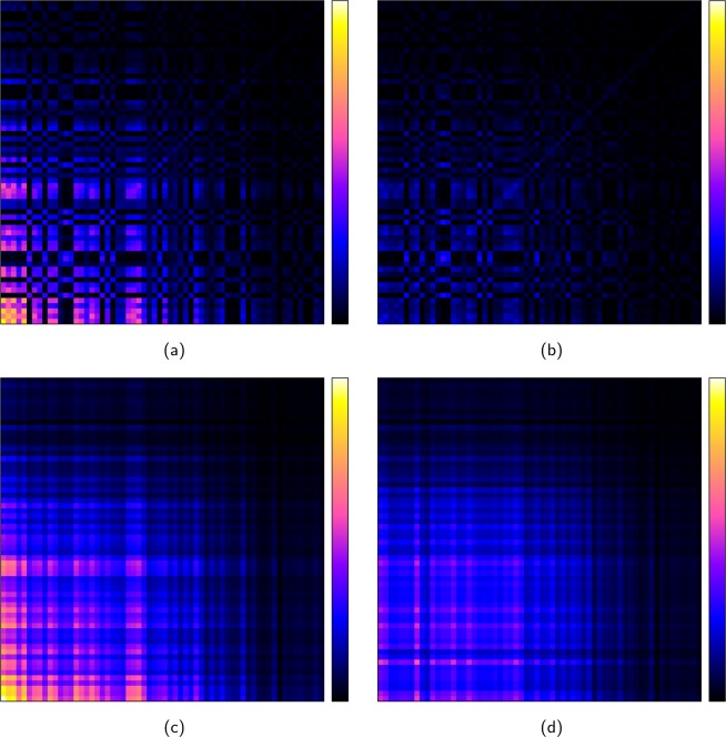
Figure 9(a,b) shows the communicability of the Dolphins network for the original dataset (Fig. 9(a)) and for the network where the links between the top 10 ranked nodes are removed (Fig. 9(b)). Clearly in this case, the communicability strongly depends on the connectivity within these 10 hubs. This dependence is also capture in the approximation of the communicability using only the properties of the hubs. Figure 9(c,d) show the approximation of communicability using the approximation of the eigenvalue–eigenvector pair from the spectral-core based on walks of length two (W2(rc, i) and Eq. (8)).
Figure 9.
Communicability for (a) the original Dolphins network and (b) when the links between the top 10 nodes are removed. (c,d) Approximation to the communicability shown in (a,b) using the approximation to the top eigenvalue-eigenvector pair from the spectral–core.
Evolution of a core
If the connectivity within the well connected nodes has such a large influence in the degree–degree correlation, how are these cores created? Recently Fire and Guestrin63 studied how the rich nodes appear and disappear in networks. They studied the evolution of 38,000 networks and noted that the creation of nodes of high degree is correlated to the speed of growth of the network. In slow growing networks the hubs appear shortly after the network becomes active and if a node becomes a hub it tends to stay a hub. In fast growing methods the hubs can appear at any time in the network evolution and their position as a top hub can change as new hubs with higher degree can appear as the network evolves.
The Barabasi–Albert (BA) model based on preferential attachment is an example of what Fire and Guestrin classify as a slow growing network. The BA model creates links between a new node and old nodes and can produce nodes with high degree. The degree of a hub is correlated with its age, nodes that becomes hubs at early stages of the network evolution, tend to remain a hub. The BA model will not produce hubs that are well interconnected, as the network evolves the rich-gets-richer mechanism increases the connectivity of the hubs but do not increase the connectivity within the hubs. It is known that network models based on the addition of new links between old nodes can have drastic changes in the overall structure of the network23,64,65. In the case that the addition of new links is biased towards connecting the hubs, i.e. the rich-club phenomenon1, then the network would have a well connected core.
An example of a non-trivial evolution of a network and its cores is in Fig. 10 which shows the number of neurones of the C. elegans from birth to maturity. The cores based on spectral properties of the network tend to grow with the network. The rich–core diminishes in size in the second spurt of growth around the 1500 time mark. The top ranked neurones are born between the 250 to 450 time mark, but there are exceptions, for example the neurone PVR is born in the 2100 time mark and ends ranked on the top 33 neurones. Around the second spurt of growth the well connected neurones increase their interconnectivity, reducing the size of the rich-core and increasing the spectral related cores. The growth of these cores correspond to an increase on the spectral radio Λ1 and an increase on the number of triangles in the network.
Figure 10.
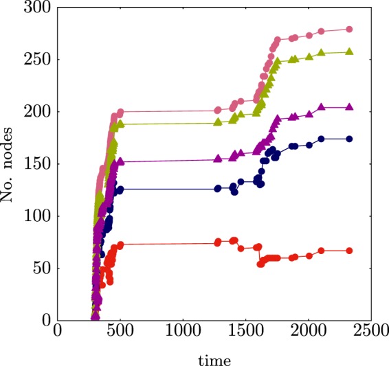
Growth of the number of neurones for the C. elegans. The top curve is the total number of neurones. From bottom to top, the rich–core, the biased–random walk, the spectral core based on walks of length two, the spectral core based on the hubs connection density and the number of neurones (pink).
There are some network growth models specifically designed to reproduce the connectivity within the well connected nodes66,67. Recently Allard and Hérbert-Dufresne68 proposed a method to construct networks ensembles based on the connectivity of a node with its k–core, their method reproduces well the long–range correlations and percolation of the network. However more research needs to be done to understand other mechanisms related to the formation of cores, in particular for fast growing networks.
Discussion
The description of a network using the degree and the connectivity with the better connected, i.e. the sequences {ki} and , produces networks with similar correlations as the original network with the advantage that the statistical description of properties related to high degree nodes are well defined even for power law networks.
The connectivity within the well connected can have a large effect on the assortativity and clustering coefficient. In the case that the network maximal degree is larger than the structural cut–off degree, changing the connectivity within the hubs has a little effect on the correlations. However it has a large effect on the number of triangles in the network. For networks that are well modelled by the degree distribution and degree–degree correlations, ensembles based on the sequences {ki} and give a good approximation to these networks. From the ensembles properties we obtained a new and tighter bound for the cut–off degree.
Another advantage describing a network via the connectivity of the hubs is that the core of a network can be defined using the connectivity within the well connected or with the well connected . The spectral and random–bias cores are based on an approximation of the spectral radius from the connectivity related to the hubs. These cores are related to the eigenvector centrality and we used them to define a new centrality measures based on the hubs relative importance. The ensembles and the cores are related as the degree–degree correlation, the clustering and the spectral radius are all related to the connectivity of the hubs, confirming the importance that the hubs play in the overall structure of the network.
Finally notice that there is an ambiguity when labelling the nodes via a degree-dependent rank. For lower degree nodes, there are many nodes with the same degree. In this case the labelling of the nodes is not unique. For high degree nodes this tend to not be a problem, as in many networks the higher degrees tend to be unique so the rank labels these nodes unambiguously. Nevertheless, it has been observed that the variation on the properties of the ensembles due to this ambiguity is very small7, which is also the case for the properties of the cores26.
Methods
Ensembles based on the rich–nodes connectivity
Maximal entropy approach
Consider a network described by the sequences {k1, …, kN} and where N is the number of nodes, L is the number of links and self–loops are not allowed. These sequences satisfy . Here we are assuming that the nodes have been ranked in decreasing order of their degree. From these sequences it is possible to construct an ensemble (or a null–model) using the Maximal Entropy approach7.
The Shannon entropy of the network is . The maximal entropy is the set of probabilities where the entropy S is maximal under certain constraints. Here the constraints are the normalisation, ∑i∑j pij = 1, the conservation of
| 17 |
and the conservation of kr
| 18 |
The common procedure to obtain the maximal entropy solution is first to label the links via the nodes labels i, j via the map ℓ = g(ij) and then transform . The constraints are expressed as where cm are M constraints that are related to qℓ via the map fm(ℓ). The solution of the maximal entropy under the constraints is obtained using the Lagrangian multipliers λ0, …, λM and the maximisation of . The maximisation of /∂qℓ = 0 for ℓ = 1, …, N(N −1)/2 gives the solution
| 19 |
This last equation combined with the constraint equations are solved to obtain the MaxEnt solution. Usually the solution of the MaxEnt is evaluated using the Partition function formalism which gives a smaller set of non-linear equations to solve. However, for the case that the constraints are the sequences {ki} and the solution can be obtained directly from Eq. (19) and the constraint conditions. The Maximal Entropy solution is given by the probabilities7
| 20 |
where
| 21 |
The values of s(n) are defined recursively with the initial condition s(1) = 1. The average number of links between nodes i and j is eij = Lpij with variance var(eij) = Lpij(1 −pij). By construction the ensemble satisfies the ‘soft’ constraints and , where the angled brackets denote expected value. The variance of the degree is .
In the following sections the ensembles ME1, ME2 and ME3 are the ones defined in the main manuscript.
Correlations
To characterise the networks produced by the ensembles we used two measures, the average neighbours degree and the assortativity coefficient.
Average neighbours degree
The average nearest neighbours degree given by 9, where is the conditional probability that given a node with degree k its neighbour has degree .
In our case pij is the probabilities obtained from on of the ensembles then
| 22 |
where if ki = k and zero otherwise.
Assortativity coefficient
The assortativity is evaluated using8
| 23 |
with
| 24 |
where ⟨…⟩ℓ is the average over all links and ⟨…⟩n is the average over all nodes. The average degree of the end nodes of a link is . Then
| 25 |
where , /2 and /2.
Some observations
Different networks can have the same assortativity coefficient ρ or average neighbours degree ⟨knn(k)⟩ but different , so there is no simple relationship between the density of connections between the rich nodes and these two measures of correlation.
Notice the value of ρ or average neighbours degree ⟨knn(k)⟩ do not define an ensemble uniquely. Figure 11(a) shows the sequence for the C. elegans and Fig. 11(b) shows the average neighbours degree for two ensembles, one obtained from the original dataset the other obtained by a modified ME2 method. The two curves are almost undistinguishable. Figure 11(c,d) shows that these ensembles have different sequences. The entropy per node of C. elegans dataset is S = 5.36 and for the other ensemble S = 5.28.
Figure 11.
(a) Average neighbours degree for the C. elegans and an ensemble with almost identical ⟨knn(k)⟩ as the original network. The percent error /Nk = 3 × 10⁻⁴, where the superscript (1) refers to the original dataset and (2) to a obtained ensemble and Nk is the number of different degrees present in the network. The sequences for (b) the original networks and (c) for the modified ME2 ensemble.
Weighted networks
For the case where the links are weighted μi and the network is described by the sequences {μi} and the maximal entropy solution is still given by Eqs (1) and (2). For the case that μi = ki and is not restricted to be an integer the degree–degree correlation tend to be ‘smoother’ than when is restricted to the integers. This shows that not also the structural cut–off degree introduces degree–degree correlations but also there are other correlations related to the discretisation of the links weights (see Fig. 12(a)).
Figure 12.
C. elegans where the degree sequence {ki} is given and all its values are integers. (a) Value of the weights obtained from the ensemble ME3 (pink) and using Eq. (26). The horizontal line is the value of ⟨knn(k)⟩ for the decorrelated network. (b) Relative error /, where is obtained from Eq. (26) and is obtained numerically from the ME3 ensemble. The rightmost vertical line corresponds to the structural cut–off , the middle vertical line is the cut–off kcut corresponding to the restrictions of the ME2 ensemble and the leftmost vertical line is kℓ corresponding to the restriction of the ensemble ME3.
Approximation to and the structural cut–off degree
If the maximal degree is less than the structural cut–off degree, the solution of probabilities in Eq. (1) can be approximated with the configuration model where pij = (kikj)/L2 and pii = 0. Notice that the configuration model satisfy the conditions that ∑j pij = ki/L and ∑i ∑jpij = 1 which are two of the constraints used for evaluating the maximal entropy solution. Using this approximation to pij in Eq. (3) we recover the well known result for uncorrelated networks knn(k) = ⟨k2⟩/⟨k⟩9.
As we are interested in the connectivity within the well connected nodes, from the configuration model the number of links that node i shares with nodes of higher rank is
| 26 |
Figure 12(b)shows the relative error / where μi was obtained numerically using ensemble ME3 for the C. elegans.
It is also possible to obtain a better approximation to the structural cut-off degree from the configuration model, using the bound that multilinks are not allowed, i.e. , then the bound is the largest value where this condition
| 27 |
still holds, the cut–off degree is .
The above structural cut–off degree assumes that the probability that a node has a self loop is small, which it would be the case multiple links between nodes are allowed. The total number of links assigned by the configuration model is given which if all the links were assigned between different nodes D = L/2. If this is not the case, to remove the degree–degree correlations due to the structural cut–off, the excess of links should be distributed as self loops. The probability that node i has a self loop is /L then the cut–off degree is given by finding the largest value such that
| 28 |
still holds, the cut–off degree is .
Table 1 shows the cut-off degree, maximal degree and assortativity of the data and the assortativity from the null model. The ME1 produces ensembles with similar correlations as the data. The ME2 and ME3 produce decorrelated ensembles if the maximal degree is lower than the cut-off degree. Notice that the structural cut–off based on the connectivity of the well connected is smaller than the cut–off based only in the configuration model, i.e. .
Table 1.
Assortativity coefficient for the ensembles of different real networks, the maximal degree and the structural cut–off degrees. The table shows the structural cut–off kcut obtained from Eq. (27), and from Eq. (28). Their values are only shown if they are smaller than the maximal degree .
| Network | ρd | ρME1 | ρME2 | ρME3 | ||||
|---|---|---|---|---|---|---|---|---|
| Adj nouns | −0.129 | −0.125 | −0.085 | −0.047 | 49 | 28 | 29.15 | 15 |
| Airports | −0.267 | −0.223 | −0.264 | −0.017 | 145 | 64 | 77.20 | 91 |
| Astro | 0.235 | 0.254 | −0.002 | 0.000 | 360 | — | — | — |
| C. elegans | −0.091 | −0.035 | −0.030 | −0.017 | 93 | 56 | 67.68 | 32 |
| Dolphins | −0.043 | −0.027 | −0.050 | −0.045 | 12 | — | — | — |
| Football | 0.162 | 0.136 | −0.024 | −0.005 | 12 | — | — | — |
| Hep-Th | 0.293 | 0.321 | −0.012 | 0.032 | 50 | — | — | — |
| AS-Internet | −0.194 | −0.188 | −0.176 | −0.042 | 2389 | 116 | 216.37 | 1334 |
| Karate | −0.475 | −0.434 | −0.205 | −0.114 | 17 | 12 | 12.49 | 12 |
| Net Sci | −0.081 | −0.025 | −0.018 | −0.010 | 34 | — | — | — |
| Political blogs | −0.221 | −0.153 | −0.046 | −0.007 | 351 | 149 | 182.86 | 116 |
| Political books | −0.127 | −0.135 | −0.021 | −0.018 | 25 | — | — | — |
| Power | 0.003 | 0.035 | −0.022 | 0.030 | 19 | — | — | — |
| Protein | −0.136 | −0.080 | −0.007 | −0.005 | 282 | 147 | 172.31 | 46 |
| Random ER | −0.004 | −0.002 | −0.012 | 0.035 | 13 | — | — | — |
| Les Mis | −0.165 | 0.005 | −0.079 | −0.065 | 36 | 19 | 22.54 | 15 |
Notice that for the Les-Mis network the ensemble ME1 has an assortativity coefficient of a decorrelated network. This network is an example where the assortativity coefficient can not give a definite answer about the degree-degree correlations, see Fig. 13. In Les-Mis network the maximal degree is larger than the structural cut–off degree so there is a correlation due to finite size effects.
Figure 13.
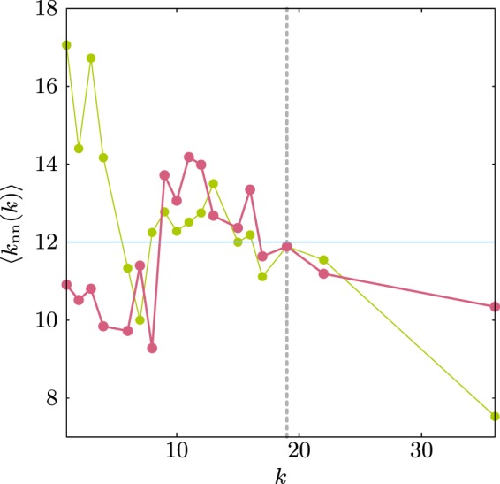
Original ⟨knn⟩ for the Les-Mis network (green) and for the ME1 ensemble (pink). Notice that in this case ρME1 = 0.005 will not capture the correlations of the ensemble. The horizontal line shows the value of the decorrelated network ⟨k2⟩/⟨k⟩ = 12.0 and the vertical line the structural cut–off degree (kcut = 19) obtained from Eq. (27).
Comment about the rich-club
Notice that the ranked based rich–club coefficient1 is , thus conserving is equivalent to the conservation of the rich–club coefficient.
The weighted ME3 model can be used to evaluate the normalised rich–club49. The uncorrelated rich–club coefficient is (using Eq. (26))
| 29 |
and the normalised weighted rich-club is
| 30 |
Clustering coefficient from the ensemble and realisation of the networks
The local clustering coefficient of node i is the number of triangles ti that contain node i normalised by the number of possible triangles that node i can have
| 31 |
In our case the probability that there is a triangle between nodes i, j and k is P(ijk) = pijpjkpki and the average number of triangles between these three nodes is ⟨tijk⟩ = L3pijpjkpki. If the network is uncorrelated then we can use the configuration model and /L3. For networks that only have degree–degree correlations the distribution pij determines the distribution of triangles and hence the clustering coefficient.
Notice that the ensembles are constructed using soft constraints, that is the constraint is on the average, that means that it is possible to have low ranking nodes (average small degree) that have many triangles. The extreme case is nodes with average degree one that nevertheless on average can be members of a triangle. This is because the chance that this kind of node has more than one link is not negligible.
Information gain using different ensembles
The information gain is measured via the Kullback–Leibler divergence, in this case it is used to measure how much information is gained if the network is described using ME1 instead of ME2 or ME3. To compare the change form ensemble ME2 to ME1 then
| 32 |
where for all i and j. This last condition is satisfied by the de–correlated ensemble. Notice that in the correlated ensemble ME1 it is possible to have , for example when i < j and (see Eq. (1)), in this case we assume that if x = 0. Table 2 shows the information gain for some real networks. The information decreases as the restrictions on the sequence are relaxed.
Table 2.
Information gain comparing the probabilities obtained from the ensembles.
| Network | |||
|---|---|---|---|
| Adj-nouns | 0.082 | 0.094 | 0.010 |
| Astro | 0.330 | 0.332 | 0.002 |
| C. elegans | 0.084 | 0.085 | 0.003 |
| Airports | 0.100 | 0.157 | 0.057 |
| Dolphins | 0.191 | 0.202 | 0.014 |
| Net. Scientists | 0.235 | 0.243 | 0.029 |
| Football | 0.106 | 0.100 | 0.009 |
| Hep-Th | 0.351 | 0.335 | 0.006 |
| AS-Internet | 0.243 | 0.366 | 0.109 |
| Karate | 0.213 | 0.232 | 0.032 |
| Les Mis | 0.184 | 0.183 | 0.011 |
| Pol. books | 0.128 | 0.133 | 0.011 |
| Power | 0.311 | 0.357 | 0.069 |
| Protein | 0.148 | 0.156 | 0.013 |
| Random Network | 0.206 | 0.224 | 0.032 |
| Pol. blogs | 0.077 | 0.083 | 0.003 |
Networks generation from the ensemble
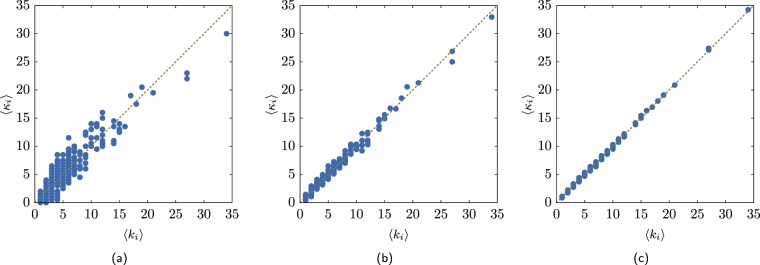
To generate a network that is a member of the ensemble we use a Bernoulli process where the existence of a link between nodes i and j is given by pij. The process is carried out until there are L links in the generated network. Figure 14(a) shows the average degree obtained from m realisations of the ensemble when multiple links are allowed.
Figure 14.
Average degree evaluated from several network realisations vs. the degree of the C. elegans network. (a) 10 realisations, (b) 100 realisations and (c) 1000 realisations.
Restricted randomisation
The other procedure to generate a network ensemble is restricted randomisation19, where the degree sequence is always fixed and the can be fixed or not. As in the ensembles generated via the maximal entropy method, the conservation of the sequences {ki} and generates networks with similar degree–degree correlations as the original network. Table 3 compares the assortativity coefficient ρ for some real networks and the average obtained from the restricted randomisations.
Table 3.
Assortativity coefficient for different networks obtained by the restricted randomisation which conserves the sequences {ki} and . The assortativity coefficient were obtained by switching links 1000 × L times.
| Network | ρ | |
|---|---|---|
| Adj nouns | −0.129 | −0.199 ± 0.014 |
| Airports | −0.267 | −0.283 ± 0.001 |
| Protein | −0.136 | −0.118 ± 0.001 |
| Random | −0.045 | −0.116 ± 0.004 |
| C. elegans | −0.092 | −0.094 ± 0.005 |
| NetSci | −0.081 | −0.101 ± 0.011 |
| AS-Internet | −0.194 | −0.195 ± 0.000 |
| Karate | −0.475 | −0.457 ± 0.018 |
| LesMis | −0.165 | −0.098 ± 0.022 |
| PolBooks | −0.127 | −0.177 ± 0.012 |
| PolBlogs | −0.221 | −0.219 ± 0.002 |
| Astro | 0.235 | 0.154 ± 0.001 |
| Football | 0.162 | 0.080 ± 0.012 |
| HepTh | 0.185 | 0.069 ± 0.004 |
| Power | 0.003 | −0.060 ± 0.005 |
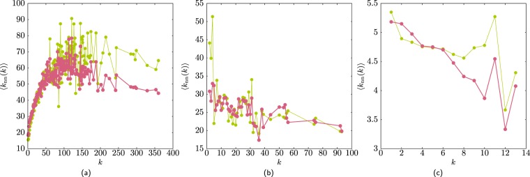
Figure 15 shows the average neighbours degree ⟨knn⟩ for several real networks, confirming that conserving the sequences {ki} and generates networks with similar degree–degree correlations. Notice that for a random network the randomisation does not generates a de-correlated network as the correlation that was present in the original network cannot be removed.
Figure 15.
Comparison of the average neighbours degree for the original network and the average obtained from the restricted randomisation. (a) The Astrophysics-collaborators, which is disassortative. (b) The C. elegans which is disassortative. (c) An a random network, which has a spurious correlation that cannot be removed by the restricted randomisation as the sequence is conserved.
Cores
Spectral cores
We assume that the nodes are ranked in decreasing order of their degree and that the networks connectivity is described by the degree sequence {ki} and the sequence . If A is the adjacency matrix where Aij = Aji = 1 if nodes i and j share a link and zero otherwise. The spectrum of the graph is the set of eigenvalues Λ1 ≥ Λ2 ≥ … ≥ ΛN of the matrix A where Λ1 is the spectral radius.
A lower bound for Λ1 is33,69, n = 1, …, where is the total number of walks of length n, A is the adjacency matrix and is a vector with all its entries equal to one. An upper bound for the number of walks is 70 where the equality is true only if n ≤ 2. The idea behind the bounds based on the hubs is to evaluate the density of walks of length one (or two) that include at least one of the hub nodes.
Bound based on walks of length one
Using the bound for Wn for n = 1 we define
The sum containing only terms of the form gives the average number of links within the top i ranked nodes. The other sum containing the terms is the average number of links between the top i ranked nodes and nodes of lower rank. Notice that if r = N then /N, and g(N) = 2L/N, which is the well known lower bound B1 = W1/W0 = 2L/N ≤ Λ1. Also notice that could be larger than g(N) = 2L/N. We split the network into two parts by considering the value r such that is maximal, that is when the density of connections between the top ranked nodes is maximal. In this case the core of the network is the nodes of rank greater than rc where
| 33 |
where the superscript in is used to label this bound. The bound is36
| 34 |
Notice that if then b1 = W1/W0 which is a well know bound of Λ1.
Bound based on walks of length two
The above bound can be improved if we consider the connectivity of the well connected nodes and the connectivity of their neighbouring nodes. In this case we consider walks of length two W2. The number of walks of length two starting from node j, W2(j), is the same as the walks of length one starting from the neighbouring nodes of j, we denote the neighbours of j as jq. Then
| 35 |
If we distinguish which walks of length 1 end on one of the top r ranked nodes then
| 36 |
where Θ(jq, r) is the step function Θ(a, b) = 1 if a < b and zero otherwise. We are interested in the first term, , which is the number of links that the nearest neighbours of j have a link with a node with rank equal of less than r, we denote this degree with . Similarly as the bound b1, we evaluate the density of these walks using
| 37 |
if
| 38 |
the bound is
| 39 |
Notice that if then b2 = W2/W0, which is the well know bound W2/.
For comparison purposes we compared these two lower bounds with the lower bounds B1 = W1/W0, and33
| 40 |
where this last bound can be expressed as a function of the assortativity coefficient ρ8,33. Also we consider the optimised bound33 based on walks of length one, two and three,
| 41 |
where
| 42 |
Notice that by construction b1 ≥ B1 and b2 ≥ B2. Table 4 compares the bounds of Λ1 for different real networks. The bound BM gives the best approximation of the Λ1 except for the Hep-Th, Power and the AS-Internet networks. However the bounds b1 and b2 are simple to evaluate and have a simple interpretation in terms of the connectivity of the network.
Table 4.
The spectral radius Λ1 and its bounds B1, B2 and B3 based on the sum of all walks of length one, two and three respectively. Bounds b1 and b2 obtained from local walks from the core, or from the local connectivity of the core nodes. The entries and are the number of nodes that constitute the core obtained from b1 and b2. The entry N is the total number of nodes in the network.
| Network | B1 | B2 | B3 | BM | b1 | b2 | Λ1 | N | ||
|---|---|---|---|---|---|---|---|---|---|---|
| Nouns | 7.58 | 10.22 | 10.94 | 12.66 | 9.30 | 11.34 | 13.15 | 49 | 66 | 112 |
| Airports | 11.92 | 25.32 | 30.49 | 44.77 | 38.02 | 42.70 | 48.07 | 71 | 71 | 500 |
| C. elegans | 16.40 | 20.62 | 21.82 | 24.58 | 17.99 | 21.22 | 25.94 | 172 | 197 | 279 |
| Dolphins | 5.12 | 5.90 | 6.17 | 6.75 | 6.04 | 6.46 | 7.19 | 41 | 39 | 62 |
| Football | 10.66 | 10.69 | 10.71 | 10.74 | 10.66 | 10.69 | 10.78 | 115 | 115 | 115 |
| Hep-Th | 4.13 | 5.99 | 7.25 | 11.00 | 9.82 | 15.05 | 23.00 | 70 | 70 | 7610 |
| Karate | 4.50 | 5.97 | 5.98 | 6.50 | 5.00 | 5.98 | 6.72 | 22 | 33 | 34 |
| Les Miss | 6.59 | 8.91 | 9.59 | 11.20 | 10.00 | 10.97 | 12.00 | 28 | 24 | 77 |
| Net Sci | 4.82 | 6.21 | 6.64 | 7.62 | 5.69 | 7.19 | 10.37 | 192 | 4 | 379 |
| Political blog | 27.31 | 47.11 | 53.21 | 69.08 | 54.45 | 63.16 | 74.08 | 323 | 321 | 1224 |
| Political book | 8.40 | 10.01 | 10.46 | 11.48 | 8.85 | 10.33 | 11.93 | 68 | 68 | 105 |
| Power | 2.66 | 3.21 | 3.42 | 3.87 | 2.88 | 4.44 | 7.48 | 3715 | 32 | 4941 |
| Protein | 6.30 | 12.34 | 13.54 | 17.38 | 12.86 | 16.79 | 21.16 | 733 | 1 | 4713 |
| AS-Internet | 4.18 | 33.35 | 28.51 | 41.81 | 20.20 | 48.97 | 60.32 | 77 | 2 | 11174 |
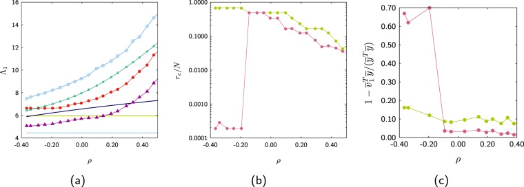
Figure 16(a) shows the behaviour of the bounds as a function of the assortativity coefficient. It seems that the bound b2 can produce better bounds that BM for networks with high assortativity or disassortativity coefficient, perhaps this is the reason that this bound is better for the Hep-Th, Power and AS-Internet networks than the BM bound. Figure 16(b) shows the size of the core obtained from the bound b1 (green) and b2 (pink). Notice the drastic change on the core size obtained from the bound b2 when the network becomes more disassortative.
Figure 16.
(a) Dependance of the different bounds as a function of the assortativity coefficient. (b) Size of the core as a function of the assortativity coefficient. (c) Relative error between the eigenvector and its approximation .
To confirm that is a bound of the spectral radius consider Rayleigh’s inequality /. If A is the adjacency matrix of a network ranked in decreasing order of its node’s degree and is a vector with 1 in the top rc entries and 0 otherwise then
 |
43 |
where is the number of links that node i shares with the rc top ranked nodes. Then is the total number of links are shared by the top rc ranked nodes, recalling that is the number of links between node i shares nodes of largest rank then . As , Rayleigh’s inequality gives .
For the bound b2, or , the procedure is similar as for the b1 case. In this case /. The entries correspond to the number of walks of length two that start in i and end in j. If is a vector with 1 in the top rc entries and 0 otherwise then, is the number of walks of length two, W2(rc, rc), that start in one of the top rc nodes and end in on of these top rc nodes. Notice that W2(rc, rc) is equal to the number of links in the whole network that connect with at least one node in rc, that is .
To measure how well the vector approximates the eigenvector we evaluate
| 44 |
where the closer this quantity is to zero, the better approximates (see Fig. 16(c)). Notice that for highly disassortative networks the size of the spectral core obtained from the bound b2 can be very small. However this is not translated into a better approximation to the eigenvector but the opposite, the approximation becomes poor.
Relationship with the eigenvector centrality
If the eigenvectors of the matrix A are and corresponding eigenvalues {Λ1, …, ΛN} where Λi ≥ Λi+1, then where ci are constants, then to first order approximation , hence is an approximation to the eigenvector centrality . The entries of are , where is the number of links that node i shares with the rc top ranked nodes. For the case of the bound considering walks of length two described by the matrix A2 the approximation to the eigencentrality is given by the vector with entries yi = W2(rc, i) where W2(rc, i) are the number of walks of length 2 that start in rc and end in any node i.
Biased random walks
Maximal rate entropy random walk (MERW)
In a finite, undirected, not bipartite and connected network a random walker would jump from node i to a neighbouring node j with a probability Pi→j. The probability that the walker is in node j at time t + 1 is pj(t + 1) = ∑i(A)ijPi→jpi(t). The probability of finding the walker in node i as time tends to infinity is given by the stationary distribution . In a network, the jump probability Pi→j can be expressed as
| 45 |
where (A)ij is the ij entry of the adjacency matrix and fj is a function of one or several topological properties of the network, in this case the stationary distribution is71
| 46 |
The measure which tell us the minimum amount of information needed to describe the stochastic walk in the network is the entropy rate /t, where St is the Shannon entropy of all walks of length t, which is
| 47 |
The maximal rate entropy corresponds to random walks where all the walks of the same length have equal probability. The value of can be expressed in terms of the spectral properties of the network as
| 48 |
For the MERW the probability Pi→j is such that all the walks of the same length have equal probability. The stationary probability for the MERW is where vi is the i entry of the eigencentrality.
Core-biased random walk
If the largest eigenvalue-eigenvector pair is not known, the MERW results suggests that a good approximation to the largest eigenvector could be used to construct a biased random walk. A bound for the largest eigenvalue in terms of the connectivity of the nodes of high degree is b1 = 1/ and an approximation to the corresponding eigenvector is , where is a vector with its top r entries equal to one and the rest to zero (see Methods: The spectral-core). The vector has entries , where is the number of links that node i shares with the top r ranked nodes.
This bound based on suggests a core biased random walk. If the top r ranked nodes are the core of the network, then a core-biased random jump is46
| 49 |
where the term 1 in the numerator and denominator has been added as it is possible that if node j has no links with the network’s core and then the random-walk will be ill-defined.
As we want to have the best possible approximation to the maximal rate entropy we define the core as the value of r which maximises the value of s(r), that is
| 50 |
where s(r) is the r dependent entropy
| 51 |
and is the stationary distribution corresponding to the core–biased random jumps of Eq. (10). The core are the nodes ranked from 1 to rc. The value of s(r) is evaluated numerically from the core biased random jump Pi→j(r) using Eq. (45) with , then evaluating the stationary distribution (via Eq. (46)) and from this distribution the rate entropy s(r) (Eq. (47)) and the rank r that maximises s(r) (Eq. (50)).
Notice that the spectral–core and the core–biased random walk, even that both are formulated as a function of the density of connections between the top ranked r nodes, there are different cores.
Table 5 shows the approximation to the maximal entropy using the core-biased random walk, the relative size of the core with respect to the network’s size and the assortativity coefficient. The relative size of the core is not related to the assortativity of the network.
Table 5.
Ratio of the core-biased entropy against the maximal entropy (sc/), relative size of the core and assortativity coefficient for some real networks.
| Network | sc/ | rc/N | ρ |
|---|---|---|---|
| Airports | 0.999 | 0.136 | -0.267 |
| CondMat | 0.945 | 0.039 | 0.157 |
| NetSci | 0.914 | 0.137 | -0.081 |
| Football | 0.998 | 0.913 | 0.162 |
| LesMis | 0.997 | 0.350 | -0.165 |
| Random | 0.983 | 0.449 | -0.045 |
| Power law | 0.972 | 0.227 | -0.004 |
| Power law | 0.970 | 0.489 | -0.245 |
| Power law | 0.980 | 0.126 | 0.222 |
| Regular | 1.000 | 1.000 | – |
Stationary probability for the core-biased random walk
The stationary distribution for the core-biased random walk is evaluated using Eq. (46) with which gives
| 52 |
which is the probability to find the random walker in node i after spending a long time visiting the network by preferring to visit nodes connected to the core.
Datasets
A description of the datasets and the dataset for the networks Karate, Dolphins, LesMis, Football, C. elgans, Net-Sci (collaboration between Network Scientists), Political blog, Political book, Power, Protein, Hep-th, AS–Internet and Astro-Ph are available from M. Newman’s web page (http://www-personal.umich.edu/~mejn/netdata/). The random network is an Erdos¨-Rényi network generated with igraph. The power law networks were also generated with igraph. The European airline network is available from Air Transportation Multiplex (http://complex.unizar.es/ãtnmultiplex/).
Author contributions
R.J.M. carried all the research presented here, wrote the main manuscript text and prepared the figures.
Competing interests
The author declares no competing interests.
Footnotes
Publisher’s note Springer Nature remains neutral with regard to jurisdictional claims in published maps and institutional affiliations.
References
- 1.Zhou S, Mondragón R. Accurately modeling the Internet topology. Phys. Rev. E. 2004;70:066108. doi: 10.1103/PhysRevE.70.066108. [DOI] [PubMed] [Google Scholar]
- 2.van den Heuvel MP, Sporns O. Rich–club organization of the human connectome. J. Neurosci. 2011;31:15775–15786. doi: 10.1523/JNEUROSCI.3539-11.2011. [DOI] [PMC free article] [PubMed] [Google Scholar]
- 3.Gleiser P. How to become a superhero. J. Stat. Mechanics: Theory and Experiment. 2007;2007:P09020. doi: 10.1088/1742-5468/2007/09/P09020. [DOI] [Google Scholar]
- 4.Xu X-K, Zhang J, Small M. Rich-club connectivity dominates assortativity and transitivity of complex networks. Phys. Rev. E. 2010;82:046117. doi: 10.1103/PhysRevE.82.046117. [DOI] [PubMed] [Google Scholar]
- 5.Xu X, Zhang J, Li P, Small M. Changing motif distributions in complex networks by manipulating rich–club connections. Physica A: Statistical Mechanics and its Applications. 2011;390:4621–4626. doi: 10.1016/j.physa.2011.06.069. [DOI] [Google Scholar]
- 6.Gollo LL, Zalesky A, Hutchison RM, van den Heuvel M, Breakspear M. Dwelling quietly in the rich club: brain network determinants of slow cortical fluctuations. Phil. Trans. R. Soc. B. 2015;370:20140165. doi: 10.1098/rstb.2014.0165. [DOI] [PMC free article] [PubMed] [Google Scholar]
- 7.Mondragón RJ. Network null-model based on maximal entropy and the rich-club. J. Complex Netw. 2014;2:288–298. doi: 10.1093/comnet/cnu006. [DOI] [Google Scholar]
- 8.Newman MEJ. Assortative mixing in networks. Phys. Rev. Lett. 2002;89:208701. doi: 10.1103/PhysRevLett.89.208701. [DOI] [PubMed] [Google Scholar]
- 9.Pastor-Satorras R, Vázquez A, Vespignani AT. Dynamical and correlation properties of the Interne. Phys. Rev. Lett. 2001;87:258701. doi: 10.1103/PhysRevLett.87.258701. [DOI] [PubMed] [Google Scholar]
- 10.Borgatti SP, Everett MG. Models of core/periphery structures. Social Networks. 2000;21:375–395. doi: 10.1016/S0378-8733(99)00019-2. [DOI] [Google Scholar]
- 11.Estrada E, Hatano N. Communicability in complex networks. Phys. Rev. E. 2008;77:036111. doi: 10.1103/PhysRevE.77.036111. [DOI] [PubMed] [Google Scholar]
- 12.Bianconi G. The entropy of randomized network ensembles. EPL (Europhysics Letters) 2007;81:28005. doi: 10.1209/0295-5075/81/28005. [DOI] [Google Scholar]
- 13.Annibale A, Coolen A, Fernandes L, Fraternali F, Kleinjung J. Tailored graph ensembles as proxies or null models for real networks i: tools for quantifying structure. Journal of Physics A: Mathematical and Theoretical. 2009;42:485001. doi: 10.1088/1751-8113/42/48/485001. [DOI] [PMC free article] [PubMed] [Google Scholar]
- 14.Bianconi G. Entropy of network ensembles. Phys. Rev. E. 2009;79:036114. doi: 10.1103/PhysRevE.79.036114. [DOI] [PubMed] [Google Scholar]
- 15.Squartini T, Garlaschelli D. Analytical maximum-likelihood method to detect patterns in real networks. New J. Phys. 2011;13:083001. doi: 10.1088/1367-2630/13/8/083001. [DOI] [Google Scholar]
- 16.Johnson S, Torres JJ, Marro J, Munoz MA. Entropic origin of disassortativity in complex networks. Phys. Rev. Lett. 2010;104:108702. doi: 10.1103/PhysRevLett.104.108702. [DOI] [PubMed] [Google Scholar]
- 17.Hou L, Small M, Lao S. Maximum entropy networks are more controllable than preferential attachment networks. Phys. Lett. A. 2014;378:3426–3430. doi: 10.1016/j.physleta.2014.09.057. [DOI] [Google Scholar]
- 18.Squartini T, Mastrandrea R, Garlaschelli D. Unbiased sampling of network ensembles. New J. Phys. 2015;17:023052. doi: 10.1088/1367-2630/17/2/023052. [DOI] [Google Scholar]
- 19.Maslov S, Sneppen K. Specificity and stability in topology of protein networks. Sci. 2002;296:910–913. doi: 10.1126/science.1065103. [DOI] [PubMed] [Google Scholar]
- 20. Mondragón, R. J. & Zhou, S. Random networks with given rich-club coefficient. Eur. Phys. J. B 85 (2012).
- 21.Squartini T, de Mol J, den Hollander F, Garlaschelli D. Breaking of ensemble equivalence in networks. Phys. Rev. Lett. 2015;115:268701. doi: 10.1103/PhysRevLett.115.268701. [DOI] [PubMed] [Google Scholar]
- 22. Ring, J. H., Young, J.-G. & Hébert-Dufresne, L. Connected graphs with a given degree sequence: Efficient sampling, correlations, community detection and robustness. In International Conference on Network Science, 33–47 (organization Springer, 2020).
- 23. Dorogovtsev, S. N. Lectures on complex networks, vol. 24 (Oxford University Press Oxford, 2010).
- 24.Bianconi G, Caldarelli G, Capocci A. Loops structure of the Internet at the autonomous system level. Phys. Rev. E. 2005;71:066116. doi: 10.1103/PhysRevE.71.066116. [DOI] [PubMed] [Google Scholar]
- 25.Bianconi G, Marsili M. Effect of degree correlations on the loop structure of scale-free networks. Phys. Rev. E. 2006;73:066127. doi: 10.1103/PhysRevE.73.066127. [DOI] [PubMed] [Google Scholar]
- 26.Ma A, Mondragón RJ. Rich-cores in networks. PloS One. 2015;10:e0119678. doi: 10.1371/journal.pone.0119678. [DOI] [PMC free article] [PubMed] [Google Scholar]
- 27.Lu X, et al. Drought rewires the cores of food webs. Nat. Climate Change. 2016;6:875–878. doi: 10.1038/nclimate3002. [DOI] [Google Scholar]
- 28. Battiston, F., Guillon, J., Chavez, M., Latora, V. & Fallani, F. D. V. Multiplex core–periphery organization of the human connectome. J. The Royal Society Interface 15, 20180514 (2018). [DOI] [PMC free article] [PubMed]
- 29.Gómez S, Arenas A, Borge-Holthoefer J, Meloni S, Moreno Y. Discrete-time markov chain approach to contact-based disease spreading in complex networks. EPL (Europhysics Letters) 2010;89:38009. doi: 10.1209/0295-5075/89/38009. [DOI] [Google Scholar]
- 30.Van Mieghem P. The N-intertwined SIS epidemic network model. Computing. 2011;93:147–169. doi: 10.1007/s00607-011-0155-y. [DOI] [Google Scholar]
- 31. Wang, Y., Chakrabarti, D., Wang, C. & Faloutsos, C. Epidemic spreading in real networks: An eigenvalue viewpoint. In 22nd International Symposium on Reliable Distributed Systems, 2003. Proceedings., 25–34 (IEEE, 2003).
- 32.Youssef M, Scoglio C. An individual-based approach to SIR epidemics in contact networks. J. Theoretical Biol. 2011;283:136–144. doi: 10.1016/j.jtbi.2011.05.029. [DOI] [PubMed] [Google Scholar]
- 33.Van Mieghem P, Wang H, Ge X, Tang S, Kuipers F. Influence of assortativity and degree-preserving rewiring on the spectra of networks. The European Physical Journal B-Condensed Matter and Complex Systems. 2010;76:643–652. doi: 10.1140/epjb/e2010-00219-x. [DOI] [Google Scholar]
- 34.D’Agostino G, Scala A, Zlatić V, Caldarelli G. Robustness and assortativity for diffusion-like processes in scale-free networks. EPL (Europhysics Letters) 2012;97:68006. doi: 10.1209/0295-5075/97/68006. [DOI] [Google Scholar]
- 35.Estrada E. Combinatorial study of degree assortativity in networks. Phys. Rev. E. 2011;84:047101. doi: 10.1103/PhysRevE.84.047101. [DOI] [PubMed] [Google Scholar]
- 36. Mondragón, R. J. Network partition via a bound of the spectral radius. Journal of Complex Networks cnw029 (2016).
- 37.Rosvall M, Bergstrom CT. Maps of random walks on complex networks reveal community structure. Proc. Natal. Acad. Sci. 2008;105:1118–1123. doi: 10.1073/pnas.0706851105. [DOI] [PMC free article] [PubMed] [Google Scholar]
- 38.Noh JD, Rieger H. Random walks on complex networks. Phys. Rev. Lett. 2004;92:118701. doi: 10.1103/PhysRevLett.92.118701. [DOI] [PubMed] [Google Scholar]
- 39.Yoon S, Lee S, Yook S-H, Kim Y. Statistical properties of sampled networks by random walks. Phys. Rev. E. 2007;75:046114. doi: 10.1103/PhysRevE.75.046114. [DOI] [PubMed] [Google Scholar]
- 40. Della Rossa, F., Dercole, F. & Piccardi, C. Profiling core-periphery network structure by random walkers. Sci. Rep. 3 (2013). [DOI] [PMC free article] [PubMed]
- 41.Burda Z, Duda J, Luck J-M, Waclaw B. Localization of the maximal entropy random walk. Phys. Rev. Lett. 2009;102:160602. doi: 10.1103/PhysRevLett.102.160602. [DOI] [PubMed] [Google Scholar]
- 42. Li, R.-H., Yu, J. X. & Liu, J. Link prediction: the power of maximal entropy random walk. In Proceedings of the 20th ACM International Conference on Information and Knowledge Management, 1147–1156 (ACM, 2011).
- 43.Ochab JK, Burda Z. Maximal entropy random walk in community detection. The European Physical Journal Special Topics. 2013;216:73–81. doi: 10.1140/epjst/e2013-01730-6. [DOI] [Google Scholar]
- 44.Yu J-G, Zhao J, Tian J, Tan Y. Maximal entropy random walk for region-based visual saliency. IEEE Transactions on Cybernetics. 2014;44:1661–1672. doi: 10.1109/TCYB.2013.2292054. [DOI] [PubMed] [Google Scholar]
- 45. Leibnitz, K., Shimokawa, T., Peper, F. & Murata, M. Maximum entropy based randomized routing in data-centric networks. In Network Operations and Management Symposium (APNOMS), 2013 15th Asia-Pacific, 1–6 (IEEE, 2013).
- 46.Mondragón RJ. Core-biased random walks in networks. J. Complex Netw. 2018;6:877–886. doi: 10.1093/comnet/cny001. [DOI] [Google Scholar]
- 47.Martin T, Zhang X, Newman M. Localization and centrality in networks. Phys. Rev. E. 2014;90:052808. doi: 10.1103/PhysRevE.90.052808. [DOI] [PubMed] [Google Scholar]
- 48.Lin Y, Zhang Z. Non-backtracking centrality based random walk on networks. The Computer Journal. 2018;62:63–80. doi: 10.1093/comjnl/bxy028. [DOI] [Google Scholar]
- 49.Colizza V, Flammini A, Serrano MA, Vespignani A. Detecting rich-club ordering in complex networks. Nature. 2006;2:110–115. [Google Scholar]
- 50.McAuley JJ, Costa LF, Caetano TS. The rich-club phenomenon across complex network hierarchies. Appl. Phys. Lett. 2007;91:084103. doi: 10.1063/1.2773951. [DOI] [Google Scholar]
- 51.Opsahl T, Colizza V, Panzarasa P, Ramasco JJ. Prominence and control: The weighted rich-club effect. Phys. Rev. Lett. 2008;101:168702. doi: 10.1103/PhysRevLett.101.168702. [DOI] [PubMed] [Google Scholar]
- 52.Serrano MA. Rich-club vs rich-multipolarization phenomena in weighted networks. Phys. Rev. E. 2008;78:026101. doi: 10.1103/PhysRevE.78.026101. [DOI] [PubMed] [Google Scholar]
- 53.Zlatic V, et al. On the rich-club effect in dense and weighted networks. The European Physical Journal B. 2009;67:271–275. doi: 10.1140/epjb/e2009-00007-9. [DOI] [Google Scholar]
- 54. Alstott, J., Panzarasa, P., Rubinov, M., Bullmore, E. T. & Vértes, P. E. A unifying framework for measuring weighted rich clubs. Sci. Rep. 4, 7258 (2014). [DOI] [PMC free article] [PubMed]
- 55.Cinelli M, Ferraro G, Iovanella A. Rich-club ordering and the dyadic effect: Two interrelated phenomena. Physica A: Statistical Mechanics and its Applications. 2018;490:808–818. doi: 10.1016/j.physa.2017.08.122. [DOI] [Google Scholar]
- 56.Cinelli M. Generalized rich-club ordering in networks. J. Complex Netw. 2019;7:702–719. doi: 10.1093/comnet/cnz002. [DOI] [Google Scholar]
- 57.de Reus MA, van den Heuvel MP. Simulated rich club lesioning in brain networks: a scaffold for communication and integration? Frontiers in Human Neuroscience. 2014;8:647. doi: 10.3389/fnhum.2014.00647. [DOI] [PMC free article] [PubMed] [Google Scholar]
- 58. Ball, G. et al. Rich-club organization of the newborn human brain. Proceedings of the National Academy of Sciences 201324118 (2014). [DOI] [PMC free article] [PubMed]
- 59.Grayson DS, et al. Structural and functional rich club organization of the brain in children and adults. PloS One. 2014;9:e88297. doi: 10.1371/journal.pone.0088297. [DOI] [PMC free article] [PubMed] [Google Scholar]
- 60.Nigam S, et al. Rich-club organization in effective connectivity among cortical neurons. The J. Neurosci. 2016;36:670–684. doi: 10.1523/JNEUROSCI.2177-15.2016. [DOI] [PMC free article] [PubMed] [Google Scholar]
- 61.Collin G, Kahn RS, de Reus MA, Cahn W, van den Heuvel MP. Impaired rich club connectivity in unaffected siblings of schizophrenia patients. Schizophrenia Bulletin. 2013;40:438–448. doi: 10.1093/schbul/sbt162. [DOI] [PMC free article] [PubMed] [Google Scholar]
- 62.Senden M, Deco G, de Reus MA, Goebel R, van den Heuvel MP. Rich club organization supports a diverse set of functional network configurations. Neuroimage. 2014;96:174–182. doi: 10.1016/j.neuroimage.2014.03.066. [DOI] [PubMed] [Google Scholar]
- 63. Fire, M. & Guestrin, C. The rise and fall of network stars: Analyzing 2.5 million graphs to reveal how high-degree vertices emerge over time. Information Processing & Management (2019).
- 64.Simon HA. On a class of skew distribution functions. Biometrika. 1955;42:425–440. doi: 10.1093/biomet/42.3-4.425. [DOI] [Google Scholar]
- 65.Bornholdt S, Ebel H. World-wide web scaling exponent from Simonas 1955 model. Phys. Rev. E. 2001;64:035104. doi: 10.1103/PhysRevE.64.035104. [DOI] [PubMed] [Google Scholar]
- 66. Zhou, S. Why the PFP model reproduces the Internet? In Communications, 2008. ICC’08. IEEE International Conference on, 203–207 (IEEE, 2008).
- 67. Csigi, M. et al. Geometric explanation of the rich-club phenomenon in complex networks. Sci. Rep. 7, 1730 (2017). [DOI] [PMC free article] [PubMed]
- 68.Allard A, Hébert-Dufresne L. Percolation and the effective structure of complex networks. Phys. Rev. X. 2019;9:011023. [Google Scholar]
- 69. Van Mieghem, P. Graph spectra for complex networks (Cambridge University Press, 2010).
- 70.Fiol MA, Garriga E. Number of walks and degree powers in a graph. Discrete Mathematics. 2009;309:2613–2614. doi: 10.1016/j.disc.2008.03.025. [DOI] [Google Scholar]
- 71. Gómez-Gardeñes, J. & Latora, V. Entropy rate of diffusion processes on complex networks. Phys. Rev. E 78, 065102 (2008). [DOI] [PubMed]


