Variable Impedance Control of Powered Knee Prostheses Using Human-Inspired Algebraic Curves

Abstract

Achieving coordinated motion between transfemoral amputee patients and powered prosthetic joints is of paramount importance for powered prostheses control. In this article, we propose employing an algebraic curve representation of nominal human walking data for a powered knee prosthesis controller design. The proposed algebraic curve representation encodes the desired holonomic relationship between the human and the powered prosthetic joints with no dependence on joint velocities. For an impedance model of the knee joint motion driven by the hip angle signal, we create a continuum of equilibria along the gait cycle using a variable impedance scheme. Our variable impedance-based control law, which is designed using the parameter-dependent Lyapunov function framework, realizes the coordinated hip-knee motion with a family of spring and damper behaviors that continuously change along the human-inspired algebraic curve. In order to accommodate variability in the user's hip motion, we propose a computationally efficient radial projection-based algorithm onto the human-inspired algebraic curve in the hip-knee plane.

1 Introduction

Coordinating the motion of transfemoral amputee patients and powered prosthetic joints is of vital importance for powered prostheses control. In order to achieve such coordinated motion patterns, the two important issues of (i) representing the human walking gait and (ii) enforcing the desired walking gait via a proper control scheme need to be addressed.

In the rehabilitation robotics literature, there are two classes of human gait cycle representation. The first class, proposed in Refs. [1]–[6], divides the gait cycle into several periods, each with their own distinct controllers. In order to enforce the desired gait motion patterns, switched impedance schemes are employed in a way that the closed-loop dynamics are forced to behave with a series of finite states consisting of passive spring and damper behaviors [1,6]. Due to the passive nature of the closed-loop dynamics, the advantage of such impedance-based schemes is the inherent stability of the interaction between the powered prosthesis and the amputee in each state of the finite state machine.

Despite the advantages of the proposed switched impedance-based strategies in Refs. [1]–[6], one shortcoming of such schemes is that they rely on nonunified representations of walking gait. Consequently, there are dozens of control parameters and transition rules that must be tuned across users and activities [5]. In order to automate the control parameter tuning procedure, techniques such as fuzzy logic-based expert systems [7] and adaptive dynamic programming [8] have been proposed in the literature. A second shortcoming stems from the fact that desynchronizing perturbations increase patient's risk of falling if the nonunified impedance-based controller switches to the wrong state with the wrong control scheme. Indeed, switched impedance-based control techniques that create isolated equilibria for the powered prosthetic joint dynamics rely on being able to estimate the precise time for switching from one finite state to another. A potential remedy for the need to determine switching times is based on creating a continuum of equilibria along the normal human walking gait and continuously evolving on the continuum, instead of having a series of isolated equilibria.

In contrast to the first class, there is a second class of wearable robot controllers that employ unified representations of the entire human gait cycle [9–16]. Unified gait controllers do not suffer the aforementioned shortcomings of the nonunified gait control schemes. In Ref. [9], the authors employed the center of pressure to unify the stance phase of the gait. Assuming a rocker foot geometry, the center of pressure-based gait in Ref. [9] is a holonomic representation of the human stance period. A holonomic gait, which separately unifies the stance phase and swing phase of walking, was proposed in Ref. [17]. The gait in Ref. [17], however, uses the patient's Cartesian coordinates as the phase variables and thus is difficult to measure with onboard sensors. In order to remove the need for measuring the patient's Cartesian coordinates, the authors in Ref. [16] have proposed two different representations using the hip angle measurement. The first one is a piecewise holonomic representation of the human walking gait cycle.

The second representation in Ref. [16], which unifies the stance and swing phases of walking, is a velocity-based (nonholonomic) gait representation using the thigh phase portrait. This second representation method was later experimentally verified in Ref. [18] via a single sensor. As another unified walking gait cycle representation, the authors in Refs. [12] and [13] proposed a thigh angle integral-based representation of walking. However, the integral term in Refs. [12] and [13] needs to be reset at the beginning of every gait cycle to prevent accumulation of drift due to variation in thigh kinematics. Furthermore, the integral-based gait in Refs. [12] and [13] cannot be used for patient's nonrhythmic motion control. In order to automate the phase-based control parameter tuning in real-time, the authors in Ref. [19] proposed using an extremum seeking control, which is run in parallel to the phase-based control scheme in Refs. [12] and [13].

Motivated by the fact that healthy hip-knee angular trajectories create closed and nonintersecting orbits during walking (see Fig. 1), we employed algebraic curves and the 3 L algorithm from the pattern recognition literature [20] to generate a unified holonomic representation of the human gait cycle in our preliminary work [21]. In particular, our human gait cycle representation, which encodes the nominal coordination between the hip and knee angles during normal level walking, is the zero set of bivariate implicit polynomials (IPs). We remark that our proposed algebraic curve fitting in Ref. [21] is closely related to the recent work in Ref. [22], where the authors use an elliptical path in the hip-knee plane to prescribe a normal walking gait for a lower limb exoskeleton during the swing phase. Our algebraic curve representation, however, unifies the entire gait cycle, including both the stance phase and the swing phase. Furthermore, unlike the elliptical path in Ref. [22], which is an open curve converging to infinity, our proposed algebraic curves are closed and bounded, which correspond to periodic human gait cycles. The closed and bounded curve properties cannot be achieved with standard one-dimensional polynomial fitting methods, as the one in Ref. [22]. In an earlier work [23], we employed a symbolic algebraic tool, which is based on computing the resultant of polynomials, for removing phase variables from autonomous bipedal robot parametric gaits. However, this approach, similar to Ref. [22], cannot be practically used for generating closed algebraic curves from human walking data due to large degrees of generated polynomials.

Fig. 1.

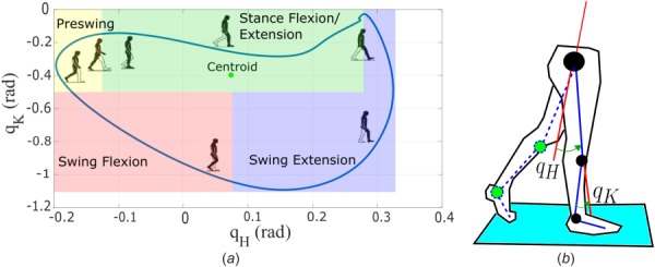
(a) Nominal human hip-knee path taken from Winter's normal cadence walking data [26], subdivided into four functional modes of stance flexion/extension, preswing, swing flexion, and swing extension and (b) the body diagram of the walking sagittal plane: $q_H$ and $q_K$ represent the hip and knee angles, respectively

Based on our preliminary work in Ref. [21], we propose employing the algebraic curve representation of nominal walking data for powered knee prosthesis controller design in this article. In order to take into account the variability that is observed during walking, we improve our earlier human-inspired algebraic curve generation algorithm in Ref. [21]. In particular, in order to take into account the fact that hip-knee walking profiles vary during walking, we employ variable geometric contraction and dilation factors, in contrast to constant values in our preliminary work. The variable contraction/dilation factor ensures that the level-sets of the generated implicit polynomials have sufficient distance from each other in a way that step-by-step variability does not significantly perturb the algebraic distance from the normal walking data. Having obtained a unified holonomic representation of walking data via algebraic curves, in the next step, we consider an impedance model of the knee joint motion driven by the hip angle signal. We then create a continuum of equilibria along the human-inspired algebraic curve using a variable impedance scheme. Our variable impedance-based control law, which is designed using the parameter-dependent Lyapunov function framework, realizes the coordinated hip-knee motion with a family of spring and damper behaviors that continuously change along the human-inspired algebraic curve. In order to accommodate the variability in user's hip motion, we propose a radial projection-based algorithm onto the human-inspired algebraic curve in the hip-knee plane. The algebraic curve representation makes the radial projection algorithm computationally efficient, with guaranteed convergence in a finite number of steps.

The rest of this paper is organized as follows: first, we briefly review preliminaries from algebraic curves and present the 3 L algorithm for fitting such curves to nominal hip-knee walking data in Sec. 2. Next, in Sec. 3, for an impedance model of the knee joint motion driven by the hip angle signal, we present our control problem formulation and demonstrate that the knee joint closed-loop dynamics take the form of a linear parameter varying (LPV) dynamical system, which is subject to disturbances that change continuously along the human-inspired algebraic curve and are dependent on the hip joint motion speed. Thereafter, in Sec. 4, we propose a parameter-dependent Lyapunov function approach for designing variable stiffness and damping gains along the human-inspired algebraic curve. Additionally, we present a radial projection-based algorithm in order to address variability in the user's hip motion and show the simulation results. In Sec. 5, we present our numerical results. Finally, we conclude this paper with final remarks and outline of possible future research directions in Sec. 6.

Notation: Given two vectors (matrices) a and b, we denote by [a; b] the vector (matrix) ${[a^{\mathrm{\top }},b^{\mathrm{\top }}]}^{\mathrm{\top }}$ where ${(·)}^{\mathrm{\top }}$ is the transpose operator. Given a square symmetric matrix X, we denote its maximum (minimum) eigenvalue by ${\lambda }_{\text{max}}(X)$ (${\lambda }_{\text{min}}(X)$).

2 3 L Algorithm for Fitting Human Data to Algebraic Curves

In this section, we review some preliminaries on algebraic curves and use the 3 L algorithm for fitting closed algebraic curves to human data. The 3 L algorithm presented in this section is an extension of the 3 L algorithm in our preliminary work in Ref. [21]. A comprehensive treatment of algebraic curves and their properties may be found in Refs. [24] and [25].

2.1 Algebraic Curves.

Algebraic curves are defined by means of bivariate IPs. Given a finite integer n, an IP

$$h(q_{\mathrm{H}},q_{\mathrm{K}})=\sum _{\mathit{ij}}{a}_{\mathit{ij}}{q}_{\mathrm{H}}^i{q}_{\mathrm{K}}^j,\hspace{1em}0\le i+j\le n$$ (1)

is a function of $q_{\mathrm{H}},\hspace{0.17em}{q}_{\mathrm{K}}$, where a_ij are real numbers. The degree of polynomial $h(q_{\mathrm{H}},q_{\mathrm{K}})$ in Eq. (1) is the maximal value of $i+j$ for which $a_{\mathit{ij}}\ne 0$. Here, we assume that IP h is of degree n. Every IP of degree n has $(n+1)(n+2)/2$ coefficients.

Given an IP $h(q_H,q_K)$ and a point $(q_{H_0},q_{K_0})$, value $h(q_{H_0},q_{K_0})$ is called the algebraic distance of the point $(q_{H_0},q_{K_0})$ to the zero set of $h(q_{H_0},q_{K_0})$. Moreover, the zero set of IP $h(q_{\mathrm{H}},q_{\mathrm{K}})$ given by Eq. (1) is defined to be

$$\mathcal{Z}(h):=\{(q_H,q_K)\in {ℝ}^2|h(q_H,q_K)=0\}$$ (2)

A real algebraic curve is the zero set of a nonzero real bivariate polynomial h. The degree of an algebraic curve is defined to be the degree of its associated bivariate implicit polynomial. Algebraic curves of degree 1, 2, 3, 4, $\dots$, are called lines, conics, cubics, quartics, $\cdots$, respectively.

Since we are interested in studying periodic human walking gait profiles, it is desirable to have closed and bounded algebraic curves. The following well-known lemma provides the necessary condition for having a closed and bounded algebraic curve.

Lemma 1. (see Ref. [25]) An algebraic curve is a closed and bounded plane curve only if it is of even degree.

2.2 3 L Algorithm for Fitting Algebraic Curves to Human Walking Data.

In this section, we fit algebraic curves to the data points obtained from a healthy gait according to Winter's normal cadence walking data [26]. Our fitting algorithm is taken from the pattern recognition literature and is known as the 3 L algorithm [20]. The 3 L algorithm presented in this section is a generalization of the algorithm in our preliminary work in Ref. [21].

2.2.1 Fitting Algebraic Curves to Human Datasets as a Quadratic Optimization Problem.

Consider an ordered, closed set, ${\mathcal{H}}_0$, of N₀ planar data points $(q_{{\mathrm{H}}_l},q_{{\mathrm{K}}_l})$. In the set ${\mathcal{H}}_0$, if $(q_{H_l},q_{K_l})$ corresponds to time instant t_l and $(q_{{\mathrm{H}}_{l+1}},q_{{\mathrm{K}}_{l+1}})$ corresponds to time instant $t_{l+1}$, then $t_l<t_{l+1}$. Here, the set ${\mathcal{H}}_0$ represents the path in the hip-knee plane, which is taken from the Winter's normal cadence walking data [26] (see Fig. 1). The set of ordered data points $(q_{{\mathrm{H}}_l},q_{{\mathrm{K}}_l}),\hspace{0.17em}1\le l\le N_0$, is the samples of the hip and knee normal cadence walking trajectories corresponding to increasing time instants during a given gait cycle. Since the walking gait profile is periodic, we have $(q_{H_1},q_{K_1})=(q_{H_{N_0}},q_{K_{N_0}})$. The geometric center or centroid of the dataset ${\mathcal{H}}_0$ is defined to be the point (see also Fig. 1)

$$p_c=[q_{\mathrm{HC}};q_{\mathrm{KC}}]:=\left[\frac{\sum _{l=1}^{N_0-1}{q}_{H_l}}{N_0-1};\frac{\sum _{l=1}^{N_0-1}{q}_{K_l}}{N_0-1}\right]$$ (3)

We would like to find an implicit bivariate polynomial $h(q_H,q_K)$ of even degree, i.e., $n=2p$ for some positive integer p, such that its zero set $\mathcal{Z}(h)$ approximates the set of human hip-knee data points ${\mathcal{H}}_0$. This approximation problem is equivalent to minimization of the error functional [20]

$$E=\sum _{(q_H,q_K)\in {\mathcal{H}}_0}{h}^2(q_H,q_K)$$ (4)

It is possible to describe the error functional E in Eq. (4) as a quadratic function of the coefficients of IP $h(q_H,q_K)$. In order to do so, we rewrite IP $h(q_H,q_K)=\sum _{\mathit{ij}}{a}_{\mathit{ij}}{q}_{\mathit{H}}^{\mathit{i}}{q}_{\mathit{K}}^{\mathit{j}}$, where $0\le i+j\le n$, using the inner-product

$$h(q_H,q_K)=m^{\mathrm{\top }}(q_H,q_K)a$$ (5)

where

$$\begin{array}{c}{m}^{\mathrm{\top }}(q_H,q_{\mathrm{K}}):=[1,\hspace{0.17em}{q}_H,\hspace{0.17em}{q}_K,\hspace{0.17em}{q}_H^2,\hspace{0.17em}{q}_H{q}_K,\hspace{0.17em}{q}_K^2,\hspace{0.17em}\cdots ,\hspace{0.17em}{q}_{\mathit{H}}^{\mathit{n}},\\ \hspace{0.17em}{q}_H^{(n-1)}{q}_K,\hspace{0.17em}{q}_H^{(n-2)}{q}_K^2,\hspace{0.17em}\cdots ,\hspace{0.17em}{q}_H{q}_K^{(n-1)},\hspace{0.17em}{q}_{\mathit{K}}^{\mathit{n}}]\end{array}$$ (6)

is a function of the two variables $q_H$ and $q_K$. Moreover

$$\begin{array}{c}a:=[a_{00},\hspace{0.17em}{a}_{10},\hspace{0.17em}{a}_{01},\hspace{0.17em}{a}_{20},\hspace{0.17em}{a}_{11},\hspace{0.17em}{a}_{02},\hspace{0.17em}\dots \\ a_{n0},\hspace{0.17em}{a}_{(n-1)1},\hspace{0.17em}{a}_{(n-2)2},\hspace{0.17em}\dots ,\hspace{0.17em}{a}_{1(n-1)},\hspace{0.17em}{a}_{0n}]\end{array}$$ (7)

is the vector of IP coefficients with

$$n_0:=(n+1)(n+2)/2$$ (8)

components. Next, using the data points $(q_{H_i},q_{K_i})\in {\mathcal{H}}_0,\hspace{0.17em}1\le i\le N_0$, we define the following matrix:

$$M_{{\mathcal{H}}_0}:=[m_1^{\mathrm{\top }};\hspace{0.17em}\cdots ;\hspace{0.17em}{m}_{N_0}^{\mathrm{\top }}]$$ (9)

where the row vectors $m_i^{\mathrm{\top }}$ are defined as $m_i^{\mathrm{\top }}:=m^{\mathrm{\top }}(q_{H_i},q_{K_i})$. It is shown in Ref. [20] that the functional E given by (4) is equal to

$$E=a^{\mathrm{\top }}{M}_{{\mathcal{H}}_0}^{\mathrm{\top }}{M}_{{\mathcal{H}}_0}a$$ (10)

Therefore, we would like to find the coefficient vector a such that the error functional E given by Eq. (10) is minimized. The direct minimization of E, which is known as the 1 L approach, often fails to generate an acceptable IP fit to a set of data points due to numerical instability problems and/or lack of physically meaningful solutions (see Refs. [20] and [27] for a detailed discussion).

2.2.2 Human Data 3L Fitting Algorithm.

Using the 3 L fitting algorithm developed in Ref. [20], we address the aforementioned numerical shortcomings of the 1 L minimization by introducing two additional datasets, which can be generated from the original human walking dataset ${\mathcal{H}}_0$. Being able to vary the two fictitious datasets on either side of the original normal cadence walking dataset ${\mathcal{H}}_0$, optimal fitting accuracies of algebraic curves to human walking data can be achieved. Furthermore, it can be shown that under suitable conditions, the algebraic curves generated by the 3 L fitting algorithm are nondegenerate [20,28,29].

Following the experimental results for pose estimation in computer graphics literature [20,25], we chose quartic algebraic curves, i.e., n = 4, to be fitted to the hip-knee normal walking data. However, there is no limitation on the degree of the algebraic curve that can be fitted to human walking datasets. The 3 L algorithm for fitting algebraic curves to human hip-knee walking data can be described in the following three steps.

2.2.2.1 Step 1: Generation of two fictitious datasets.

Given that the dataset ${\mathcal{H}}_0$, representing the nominal human walking gait in the hip-knee plane [26], introduces two fictitious datasets close to ${\mathcal{H}}_0$. The first set, which is denoted by ${\mathcal{H}}_{+}$ and is located outside the dataset ${\mathcal{H}}_0$, has $N_{+}$ points and corresponds to the algebraic distance c (see Sec. 2.1 for the definition of algebraic distance), where c is a design parameter to be chosen. The second fictitious dataset, which is denoted by ${\mathcal{H}}_{-}$ and is located inside the dataset ${\mathcal{H}}_0$, has $N_{-}$ points and corresponds to the algebraic distance—c. In this article, we have chosen the design parameter to be c = 1.

In order to generate the two fictitious datasets ${\mathcal{H}}_{+}$ and ${\mathcal{H}}_{-}$ in this article, we translated the centroid or the geometric center of the dataset ${\mathcal{H}}_0$ given by Eq. (3) to the origin of the $q_H-q_K$ plane. In particular, we translated the original dataset to obtain

$${\mathcal{H}}_0^t=\{\left[\begin{array}{c}{q}_H\\ q_K\end{array}\right]-\left[\begin{array}{c}{q}_{\mathrm{HC}}\\ q_{\mathrm{KC}}\end{array}\right]:\left[\begin{array}{c}{q}_H\\ q_K\end{array}\right]\in {\mathcal{H}}_0\}$$ (11)

where ${[q_{\mathrm{HC}},\hspace{0.17em}{q}_{\mathrm{KC}}]}^{\mathrm{\top }}$ is the centroid of the human dataset ${\mathcal{H}}_0$.

In our preliminary work in Ref. [21], we scaled the translated dataset ${\mathcal{H}}_0^t$ by constant scaling factors ${\alpha }_{+}>1$ and $0<{\alpha }_{-}<1$ to generate ${\mathcal{H}}_{+}$ and ${\mathcal{H}}_{-}$, respectively. The multiplication of the translated dataset ${\mathcal{H}}_0^t$ by ${\alpha }_{+}$ and ${\alpha }_{-}$ corresponds to geometric contraction and geometric dilation, respectively. For the presented results in Ref. [21], we chose ${\alpha }_{+}=1.02$ and ${\alpha }_{-}=0.98$.

In this article, we employ variable geometric contraction and dilation factors in order to take into account the fact that hip-knee walking profiles vary during walking. The variable contraction/dilation factor ensures that the level-sets of the generated IP $h^{\mathrm{\star }}(·)$ have sufficient distance from each other in a way that step-by-step variability does not significantly perturb the algebraic distance from the zero level-set of $h^{\mathrm{\star }}(·)$. In order to take into account the aforementioned variability, we have chosen the two radial basis functions (RBFs)

$${\alpha }_{\pm }\left(l\right)={\alpha }_{\pm }+\Delta {\alpha }_{1\pm }\hspace{0.17em}\text{exp}\left(\frac{-{\left(\frac{l-l_1}{N}\right)}^2}{{\beta }_1^2}\right)+\Delta {\alpha }_{2\pm }\hspace{0.17em}\text{exp}\left(\frac{-{\left(\frac{l-l_2}{N}\right)}^2}{{\beta }_2^2}\right)$$ (12)

as our geometric contraction/dilation factors. In Eq. (12), ${\alpha }_{\pm }$ are the constant factors used in Ref. [21], the samples l₁ and l₂ correspond to the walking data at 50% and 75% of the gait cycle, and $\Delta {\alpha }_{1\pm }$ and $\Delta {\alpha }_{2\pm }$ enlarge the distance between the two fictitious datasets with ${\mathcal{H}}_0$.

The end results of the first step are the two datasets

$${\mathcal{H}}_{\pm }=\left\{{\alpha }_{\pm }(l)\left(\left[\begin{array}{c}{q}_H(l)\\ q_K(l)\end{array}\right]-\left[\begin{array}{c}{q}_{\mathrm{HC}}\\ q_{\mathit{CC}}\end{array}\right]\right):\left[\begin{array}{c}{q}_H(l)\\ q_K(l)\end{array}\right]\in {\mathcal{H}}_0\right\}$$ (13)

Remark 1. In steps 2 and 3, we consider ${\mathcal{H}}_0^t$ and ${\mathcal{H}}_{\pm }$ in Eqs. (11) and (13), respectively, whose geometric centers are located at the origin of the $q_H-q_K$ plane. In the final step, the generated algebraic curve needs to be translated back to the geometric center of human dataset ${\mathcal{H}}_0$.

2.2.2.2 Step 2: Defining the three level-set matrix.

Define the three level-set (3L) matrix

$$M_{3L}:=\left[\begin{array}{c}{M}_{{\mathcal{H}}_{-}}\\ M_{{\mathcal{H}}_0^t}\\ M_{{\mathcal{H}}_{+}}\end{array}\right]\in {\Re }^{(N_{+}+N_0+N_{-})\times n_0}$$ (14)

where n₀ is the number of coefficients of IP h given by Eq. (8). In Eq. (14), the matrices $M_{{\mathcal{H}}_0^t}$, $M_{{\mathcal{H}}_{+}}$, and $M_{{\mathcal{H}}_{-}}$ are defined as

$$M_{{\mathcal{H}}_0^t}:=\left[\begin{array}{c}{m}^{\mathrm{\top }}(q_{H_1}^t,q_{K_1}^t)\\ \cdots \\ m^{\mathrm{\top }}(q_{H_{N_0}}^t,q_{K_{N_0}}^t)\end{array}\right],M_{{\mathcal{H}}_{\pm }}:=\left[\begin{array}{c}{m}^{\mathrm{\top }}(q_{H_1}^{\pm },q_{K_1}^{\pm })\\ \cdots \\ m^{\mathrm{\top }}(q_{H_{N_{\pm }}}^{\pm },q_{K_{N_{\pm }}}^{\pm })\end{array}\right]$$ (15)

where the points $(q_{H_l}^t,q_{K_l}^t),\hspace{0.17em}1\le l\le N_0$, belong to the dataset ${\mathcal{H}}_0^t$ given by Eq. (11). Similarly, the points $(q_{H_{l_{\pm }}}^{\pm },q_{K_{l_{\pm }}}^{\pm }),1\le l_{\pm }\le N_{\pm }$, belong to the two fictitious datasets in Eq. (13).

2.2.2.3 Step 3: Solving for the unknown implicit polynomials coefficients.

Define the $(N_{+}+N_0+N_{-})$ component column vector of algebraic distances

$$b:=[-c\hspace{0.17em}{1}_{N_{-}};\hspace{0.17em}01_{N_0};\hspace{0.17em}c\hspace{0.17em}{1}_{N_{+}}]$$ (16)

where ${\mathbb{1}}_k$, for a given integer k, is a column vector of ones belonging to ${ℝ}^k$. Consider equation $M_{3L}a=b$, with $M_{3L}$ given by Eq. (14) and b given by Eq. (16). Computing the pseudo-inverse solution for the coefficient vector a, we have

$$a^{\mathrm{\star }}={(M_{3L}^{\mathrm{\top }}{M}_{3L})}^{-1}{M}_{3L}^{\mathrm{\top }}b$$

The algebraic curve fitted to the human data is the zero set of

$$h^{\mathrm{\star }}(q_H,q_K)=m^{\mathrm{\top }}(q_H-q_{\mathrm{HC}},\hspace{0.17em}{q}_K-q_{\mathrm{KC}})a^{\mathrm{\star }}$$ (17)

where $m^{\mathrm{\top }}(·,·)$ is the function defined by Eq. (6) and $p_{\mathrm{c}}={[q_{\mathrm{HC}},\hspace{0.17em}{q}_{\mathrm{KC}}]}^{\mathrm{\top }}$ is the centroid of the human dataset ${\mathcal{H}}_0$. The translation in Eq. (17) corresponds to translation of the geometric center of the obtained algebraic curve from the origin to the human dataset centroid, as explained in Remark 1. The human-inspired IP $h^{\mathrm{\star }}(q_H,q_K)$ represents a desired implicit relationship between the human's hip angle and the wearable robot knee angle. As the human's hip angle $q_H(t)$ evolves with time, driving $h^{\mathrm{\star }}(q_H(t),q_K)$ to zero via feedback corresponds to coordinating the motion of the knee with the hip during level walking according to the human walking closed curve in Fig. 1. The algebraic curve given by IP $h^{\mathrm{\star }}(q_H,q_K)$ represents a holonomic relationship as it only depends on the joint angles $q_H$ and $q_K$, as opposed to the joint angle velocities.

2.2.3 Discussion of the Obtained Algebraic Curve Fits.

Using the 3 L algorithm with two different types of fictitious datasets, we obtained two quartic IPs whose zero level sets are depicted in Fig. 2. Figure 2(a) corresponds to choosing variable geometric factor functions while Fig. 2(b) corresponds to choosing a constant geometric factor coefficient in step 1 of our algorithm. As it can be seen from Fig. 2, the shape of the level sets and their values at different configurations differ from each other in Figs. 2(a) and 2(b). Moreover, the level sets in Fig. 2(a), which is based on the improvement over our preliminary work in Ref. [21], are further from each other during the stance to swing phase transition. Furthermore, if the hip-knee configurations are located further from the nominal Winter's walking data [30], the level set values in Fig. 2(a) in comparison with Fig. 2(b) do not grow very large.

Fig. 2.

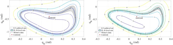
The quartic algebraic curves fitted to Winter's normal cadence walking data [26]. (a) and (b) correspond to the variable and constant dilation/contraction geometric factors, respectively. In both figures, the dashed curve represents the Winter's normal cadence walking. The level sets of IP $h^{\mathrm{\star }}(q_H,q_K)$ are labeled with their corresponding algebraic distance in the figure. The gray band around the zero set of IP $h^{\mathrm{\star }}(q_H,q_K)$ corresponds to the hip and knee configurations that belong to sublevel set $\{(q_H,q_K):|h^{\mathrm{\star }}(q_H,q_K)|\le c_0\}$, where $c_0=0.5$.

The largest deviation of the quartic algebraic curve fits from Winter's normal cadence walking data, for both of the fits, happens during the stance flexion/extension phase at around the configuration ${[0.2677\hspace{0.17em}\text{rad},-0.081\hspace{0.17em}\text{rad}]}^{\mathrm{\top }}$, where the knee angle deviates from the nominal value by around $0.04\hspace{0.17em}\text{rad}\approx 2.3\hspace{0.17em}\mathrm{deg}$ for both the cases. The gray band around the zero set of IP $h^{\mathrm{\star }}(q_H,q_K)$ corresponds to the hip and knee configurations that belong to the sublevel set $\{(q_H,q_K):|h^{\mathrm{\star }}(q_H,q_K)|\le c_0\}$ associated with the algebraic distance $c_0=0.5$. As it can be seen from Fig. 2, the level sets of the fitted IPs $h^{\mathrm{\star }}(q_H,q_K)$ do not intersect with each other, corresponding to the fact that the generated algebraic curves are nondegenerate. Furthermore, as the algebraic distances from the zero set $\mathcal{Z}(h^{\mathrm{\star }})$ change in a small manner, the joint angles do not deviate drastically from the nominal values. This continuity feature is desirable for controller design; since for small values of $|h^{\mathrm{\star }}(q_H,q_K)|$, the hip-knee configurations are still close to the fitted algebraic curve.

3 Control Problem Formulation

In this section, we consider an impedance model of the knee joint motion driven by the hip angle signal. Our control problem formulation is motivated by the approach in Refs. [1] and [6], where the impedance-based feedback control is employed to render the closed-loop dynamics of the powered prosthetic joints as a series of passive spring and damper behaviors. Due to the passive nature of the closed-loop dynamics under impedance-based control laws, the interaction between the powered prosthesis and the amputee will be inherently stable. However, we depart from the control framework in Refs. [1] and [6] by creating a continuum of equilibria along the human-inspired algebraic curve instead of having a series of isolated equilibria. As it will be shown in this section, the resulting closed-loop knee joint motion can be described by a LPV dynamical system.

We consider the impedance model

$$J_{\text{kn}}{\ddot{q}}_K+b_{\text{kn}}{\dot{q}}_K+k_{\text{kn}}{q}_K=u$$ (18)

for the knee joint motion, where u is the torque applied to the powered knee prosthesis. Furthermore, we let the polar representation of the human-inspired algebraic curve in Eq. (17) be

$$\left[\begin{array}{c}{q}_H^{*}(\sigma )\\ q_K^{*}(\sigma )\end{array}\right]=\left[\begin{array}{c}r(\sigma )\text{cos}(\sigma )+q_{\mathrm{HC}}\\ r(\sigma )\text{sin}(\sigma )+q_{\mathrm{KC}}\end{array}\right]$$ (19)

where the polar angle σ at each point $(q_H^{*},q_K^{*})$ on the human-inspired algebraic curve is given by

$$\sigma =\arctan 2(q_K^{*}-q_{\mathrm{KC}},\hspace{0.17em}{q}_H^{*}-q_{\mathrm{HC}})$$ (20)

Whenever the hip joint evolves according to the normal human walking gait, i.e., when $q_H(t)=q_H^{*}(\sigma (t))$, driving the output $h^{\mathrm{\star }}(q_H(t),q_K(t))$ to zero or sufficiently close to zero will coordinate the motion of the knee with the driving hip angle signal according to the human-inspired algebraic curve in Fig. 1. One way to achieve this objective is to make the knee tracking error

$$e(\sigma (t)):=q_K(t)-q_K^{*}(\sigma (t))$$ (21)

converge to zero or become sufficiently small along the algebraic curve. Furthermore, we would like that whenever the amputee stops moving his/her hip at $q_H=q_H^{*}(\sigma )$, the knee joint comes to rest at $q_K=q_K^{*}(\sigma )$. From the aforementioned discussion, we would like to create the following continuum of equilibria:

$$x_e(\sigma ):=\left[\begin{array}{c}{q}_K^{*}(\sigma )\\ 0\end{array}\right]$$ (22)

for the knee dynamics along the human-inspired algebraic curve. As it can be seen from Eq. (22), the continuum of equilibria is parameterized by the polar angle σ.

In order to derive the knee error dynamics along the continuum of equilibria $x_e(\sigma )$, where $x:={[q_K,\hspace{0.17em}{\dot{q}}_K]}^{\mathrm{\top }}$, we define

$$x_{\delta }(t):=x(t)-x_{\mathrm{e}}(\sigma (t))$$

and take its time derivative to obtain

$${\dot{x}}_{\delta }=A{x}_{\delta }+\mathit{Bu}+d_{\mathrm{e}}(\sigma ,\dot{\sigma })$$ (23)

where

$$A:=[0,\hspace{0.17em}\hspace{0.17em}1;\hspace{0.17em}\frac{-k_{\text{kn}}}{J_{\text{kn}}},\hspace{0.17em}\hspace{0.17em}\frac{-b_{\text{kn}}}{J_{\text{kn}}}],\hspace{1em}B:=[0;\hspace{0.17em}\frac{1}{J_{\text{kn}}}]$$ (24)

and

$$d_{\mathrm{e}}(\sigma ,\dot{\sigma }):=-\frac{\partial x_{\mathrm{e}}(\sigma )}{\partial \sigma }\dot{\sigma }$$ (25)

As the polar angle σ evolves along the human-inspired algebraic curve, we let our control input take the form

$$u(\sigma )=-u_{\delta }-u_e(\sigma )$$ (26)

where $u_{\mathrm{e}}(\sigma ):=(k_{\text{kn}}/J_{\text{kn}})q_K^{*}(\sigma )$. The control input $u_{\mathrm{e}}(\sigma )$ renders $x_e(\sigma )$ an equilibrium for the knee joint dynamics.

In order to completely determine the form of our feedback control scheme, we use the variable state feedback control law

$$u_{\delta }=K_{\mathrm{c}}(\sigma )x_{\delta }$$ (27)

Under the control law in Eqs. (26) and (27), the error dynamics of the prosthetic knee joint motion become

$${\dot{x}}_{\delta }=A_{\text{cl}}(\sigma )x_{\delta }+d_{\mathrm{e}}(\sigma ,\dot{\sigma })$$ (28)

where $A_{\text{cl}}(\sigma ):=A-B{K}_{\mathrm{c}}(\sigma ).$

Creating a continuum of equilibria via the feedback control law in Eqs. (26) and (27) along the human-inspired algebraic curve renders the knee closed-loop error dynamics a LPV system

$${\dot{x}}_{\delta }=A_{\text{cl}}(\sigma )x_{\delta }$$ (29)

subject to disturbances of the form $d_{\mathrm{e}}(\sigma ,\dot{\sigma })$ given by Eq. (25). Under the condition of frozen equilibria, i.e., whenever the hip comes to rest, we have $\dot{\sigma }=0$. Consequently, from Eq. (25), it follows that $d_{\mathrm{e}}(\sigma ,\dot{\sigma })=0$. Therefore, under the frozen equilibria condition, the knee closed-loop error dynamics take the LPV form given by Eq. (29).

Remark 2. The polar angle σ in Eq. (20), which is defined using the human-inspired algebraic curve, can be viewed as a gain scheduling variable (see, e.g., Ref. [31]) that parameterizes the continuum of equilibria for the powered knee prosthesis dynamics.

4 Variable Impedance Control Design

Having formulated our control problem in Sec. 3, we first provide a parameter-dependent Lyapunov function approach for designing variable impedance gains along the human-inspired algebraic curve in Sec. 4.1. The results in Sec. 4.1 are applicable when the human hip evolves according to a nominal gait profile on the algebraic curve. In order to address variability in the user's hip motion, we present a radial projection-based algorithm in Sec. 4.2.

4.1 Variable Impedance Control Design Using Parameter Dependent Lyapunov Functions.

In this section, we assume that the hip joint evolves, with a bounded rate of change, along the algebraic curve according to $q_H(t)=q_H^{*}(\sigma (t))$, where $q_H^{*}(\sigma )$ is given by the polar representation in Eq. (19). Under this assumption, we would like to make the tracking error in Eq. (21) practically stable [32]. Practical stability of the error dynamics means that the error can be made arbitrarily small via a proper choice of the state feedback gain $K_{\mathrm{c}}(\sigma )$.

We consider the impedance-based variable state feedback

$$K_c(\sigma )=[K_p(\sigma ),\hspace{0.17em}{K}_d(\sigma )]$$ (30)

where the variable stiffness $K_p(\sigma )$ and the variable damping $K_d(\sigma )$ are some smooth functions of σ, which continuously vary along the human-inspired algebraic curve.

Since the variable σ is an angular variable, the stiffness function $K_p(\sigma )$ and the damping function $K_d(\sigma )$ need to be $2\pi$-periodic functions of σ. In other words, we need to have

$$K_p(\sigma +2\pi )=K_p(\sigma ),\hspace{1em}\hspace{0.17em}{K}_d(\sigma +2\pi )=K_d(\sigma )$$ (31)

for all values of σ.

Under Eq. (30), the control law given by Eqs. (26) and (27) takes the form

$$u(\sigma )=K_p(\sigma )e(\sigma )+K_d(\sigma ){\dot{q}}_K-u_e(\sigma )$$ (32)

where $e(\sigma )$ is given by Eq. (21). The obtained control law $u(\sigma )$ in Eq. (32) is a variable impedance control law that does not depend on a reference velocity, e.g., on ${\dot{q}}_K^{*}(\sigma )$. Additionally, under the proposed control law in Eq. (32), the closed-loop state matrix takes the form

$$A_{\text{cl}}(\sigma )=[0,\hspace{0.17em}1;-a_p(\sigma ),-a_d(\sigma )]$$ (33)

where

$$a_p(\sigma ):=K_p(\sigma )+\frac{k_{\text{kn}}}{J_{\text{kn}}},\hspace{1em}{a}_d(\sigma ):=K_d(\sigma )+\frac{b_{\text{kn}}}{J_{\text{kn}}}$$

Since the stiffness $K_p(\sigma )$ and the damping $K_d(\sigma )$ functions are $2\pi$-periodic by design, it follows that the closed-loop state matrix $A_{\text{cl}}(\sigma )$ satisfies the periodicity condition $A_{\text{cl}}(\sigma +2\pi )=A_{\text{cl}}(\sigma )$, for all values of the angular variable σ.

In order to study the stability of the LPV closed-loop dynamics of the knee joint motion, we use a well-established class of Lyapunov functions, called the parameter-dependent Lyapunov functions [33]. In particular, we consider the following parameter-dependent Lyapunov candidate function:

$$V(x_{\delta },\sigma ):=x_{\delta }^{\mathrm{T}}X(\sigma )x_{\delta }$$ (34)

where $X(\sigma )$ is a symmetric and positive definite matrix, which is parameterized by the polar angle σ. Furthermore, since σ is an angular variable, the matrix $X(\sigma )$ should be chosen to satisfy the periodicity condition $X(\sigma +2\pi )=X(\sigma )$, for all values of σ.

As it can be seen from Eq. (34), the parameter-dependent Lyapunov function $V(x_{\delta },\sigma )$ is not only a function of the states of the powered prosthesis but also a periodic function of the polar angle variable σ, which determines where the knee joint should be located along the human-inspired algebraic curve. In order to proceed further, we take the derivative of $V(x_{\delta },\sigma )$ along the trajectories of Eq. (28) and obtain

$$\begin{array}{c}\dot{V}(x_{\delta },\sigma ):=x_{\delta }^{\mathrm{\top }}\{X(\sigma )A_{\text{cl}}(\sigma )+A_{\text{cl}}^{\mathrm{\top }}(\sigma )X(\sigma )+\dot{X}(\sigma )\}{x}_{\delta }+2x_{\delta }^{\mathrm{\top }}X(\sigma )d_{\mathrm{e}}(\sigma ,\dot{\sigma })\end{array}$$ (35)

From Eq. (20), it follows that $|\sigma (t)|\le 2\pi$, for all time instants t. We also assume that the rate of change of the polar angle satisfies

$$|\dot{\sigma }(t)|\le \mathrm{\rho }$$ (36)

for all time instants t, where ρ is a positive constant. Under the bounded rate of change condition in Eq. (36), the disturbance term given by Eq. (25) satisfies

$$\left|\right|d_e(\sigma ,\dot{\sigma })\left|\right|\le \mathrm{\rho }\left|\frac{d{q}_K^{*}(\sigma )}{d\sigma }\right|,\hspace{0.17em}\hspace{0.17em}\text{for}\hspace{0.17em}\text{all}\hspace{0.17em}\sigma$$ (37)

The values of $|d{q}_K^{*}(\sigma )/d\sigma |$, which will be used for designing the variable impedance gains later, are depicted versus the percentage of stride in Fig. 3.

Fig. 3.

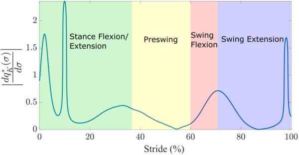
The values of $|d{q}_K^{*}(\sigma )/d\sigma |$ versus the percentage of stride

When the rate of change of the variable σ is bounded but an upper bound is not known a priori, the following proposition provides a stability condition, based on a Lyapunov matrix inequality.

Proposition 1. Consider the closed-loop dynamics in Eqs. (28) and (33) and assume that the matrix $X(\sigma )$ in Eq. (34) is equal to a symmetric and positive definite constant matrix X. Furthermore, assume that the rate of change of the variable σ is bounded by $|\dot{\sigma }(t)|\le \mathrm{\rho }$ for some unknown constant ρ. If the Lyapunov inequality

$$Q(\sigma ):=X{A}_{\text{cl}}(\sigma )+A_{\text{cl}}^{\mathrm{\top }}(\sigma )X<0$$ (38)

is satisfied for all σ, then,

• (i)the continuum of equilibria parameterized by σ in Eq. (22) is exponentially stable under $\dot{\sigma }=0$; and,
• (ii)
  when $\dot{\sigma }\ne 0$, the error $x_{\delta }(t)$ is bounded according to

  $$V\left(x_{\delta }\right(t),\sigma (t\left)\right)\le V\left(x_{\delta }\right(0),\sigma (0\left)\right)\text{exp}(-\zeta (\sigma \left)t\right)+\frac{{\left(d{q}_K^{*}\right(\sigma )/d\sigma )}^2}{\zeta (\sigma )}{\mathrm{\rho }}^2$$ (39)

  for all time instants t > 0, where $\zeta (\sigma ):=\frac{{\lambda }_{\text{min}}(Q(\sigma ))}{{\lambda }_{\text{max}}(X)}-{\lambda }_{\text{max}}(X)$.

Proof. We provide a sketch of the proof. From the inequality in Eq. (38) and since the matrix $X(\sigma )=X$ is constant, it follows that:

$$\dot{V}(x_{\delta },\sigma )\le -x_{\delta }^{\mathrm{\top }}Q{x}_{\delta }+2x_{\delta }^{\mathrm{\top }}X{d}_e(\sigma ,\dot{\sigma })$$

Therefore, since $d_e(\sigma ,\dot{\sigma })=0$ when $\dot{\sigma }=0$, (i) follows. Statement (ii) follows from a direct application of the comparison lemma [34] to the above inequality. $\mathrm{■}$

Proposition 1 provides conditions that can be used for designing the variable stiffness and damping gains along the human-inspired algebraic curve. From standard results in the nonlinear systems literature (see, e.g., Theorem 4.6 in Ref. [34]), the Lyapunov matrix inequality in Eq. (38) is satisfied if and only if for all σ the eigenvalues of the matrix $A_{\text{cl}}(\sigma )$ given by Eq. (33) are located in the open left-half complex plane. This objective will be achieved if and only if $a_p(\sigma )>0$ and $a_d(\sigma )>0$ for all values of σ. As it will be discussed in Sec. 5, attenuation of the disturbance $d_e(·)$ in Eq. (23), which exists due to continuous movement of the operating equilibrium point along the algebraic curve during walking, will be achieved if both impedance gains $K_p(\sigma )$ and $K_d(\sigma )$ change continuously with $\left|\right|d_e(·)\left|\right|$ along the algebraic curve.

In order to design the variable impedance gains, we also need to express them in a periodic basis function. Motivated by the fact that extensive numerical techniques for parameter-dependent Lyapunov functions have been developed using polynomials (see, e.g., Refs. [31] and [33]), we propose using periodic Bézier polynomials for parameterization of our variable stiffness and damping gains. We remark that Bézier polynomials have been extensively used for encoding the continuous periodic motion of underactuated mechanical systems as well as the stable walking gaits of autonomous bipedal robots that are subject to impulsive ground contact forces [35–37]. From the aforementioned discussion, we propose using the Bézier polynomial parameterizations

$$\begin{array}{c}{K}_p(\sigma )=\frac{1}{2\pi }\sum _{i=0}^{N_{\mathrm{p}}}{k}_{p,i}\left(\begin{array}{c}{N}_p\\ i\end{array}\right){\sigma }^i{(2\pi -\sigma )}^{(N_p-i)}\\ K_d(\sigma )=\frac{1}{2\pi }\sum _{i=0}^{N_{\mathrm{d}}}{k}_{d,i}\left(\begin{array}{c}{N}_d\\ i\end{array}\right){\sigma }^i{(2\pi -\sigma )}^{(N_d-i)}\end{array}$$ (40)

for the variable impedance gains. In Eq. (40), $N_p,\hspace{0.17em}{k}_{p,i}$, and $N_d,\hspace{0.17em}{k}_{d,i}$ are the degrees and coefficients of the Bézier polynomials, respectively. Due to the periodicity conditions in Eq. (31), it follows that the following equality constraints should be satisfied:

$$k_{p,0}=k_{p,N_p},\hspace{1em}{k}_{d,0}=k_{d,N_d}$$ (41)

4.2 Extension of Control Design Under Variability in the User's Hip Motion.

Under the nominal hip joint motion, i.e., when $q_H(t)=q_H^{*}(\sigma (t))$, the reference knee joint angle is given by $q_K(t)=q_K^{*}(\sigma (t))$ such that the pair $(q_H^{*}(\sigma (t)),q_K^{*}(\sigma (t)))$ belongs to the human inspired algebraic curve, i.e., $h^{\mathrm{\star }}(q_H^{*}(\sigma (t)),q_K^{*}(\sigma (t)))=0$. However, when the user's hip motion undergoes variability and is no longer given by the nominal function $q_H=q_H^{*}(\sigma )$, determining the reference knee joint angle for the variable impedance scheme will become nontrivial.

Under the hip motion variability, the pair $p(t):=(q_H(t),q_K(t))$ no longer belongs to the human-inspired algebraic curve. However, if p(t) evolves in a neighborhood of $\mathcal{Z}(h^{\mathrm{\star }})$, it is possible to project it onto the human-inspired algebraic curve and obtain the reference point

$$(q_H^{*}(t),q_K^{*}(t)):={\pi }_{\mathcal{Z}(h^{\mathrm{\star }})}(p(t))$$ (42)

where ${\pi }_{\mathcal{Z}(h^{\mathrm{\star }})}:{ℝ}^2\to \mathcal{Z}(h^{\mathrm{\star }})$ is a proper projection mapping, to be designed, onto the human-inspired algebraic curve.

A proper projection mapping ${\pi }_{\mathcal{Z}(h^{\mathrm{\star }})}$, which provides the reference points on the human-inspired algebraic curve during walking, should enjoy several properties: (i) for each complete revolution of the pair $p(t)=(q_H(t),q_K(t))$ on a closed curve in a neighborhood of the human-inspired algebraic curve, the projected point ${\pi }_{\mathcal{Z}(h^{\mathrm{\star }})}(p(t))$ should undergo a complete revolution on the human-inspired algebraic curve $\mathcal{Z}(h^{\mathrm{\star }})$; (ii) each point on the human-inspired algebraic curve should be mapped onto itself via the projection mapping, i.e., ${\pi }_{\mathcal{Z}(h^{\mathrm{\star }})}(p)=p$ for all $p\in \mathcal{Z}(h^{\mathrm{\star }})$; and (iii) the projection mapping computation should be fast enough for control implementation purposes.

Using the geometrical structure that is afforded by the human-inspired algebraic curve representation of the gait cycle, we propose a radial projection mapping candidate. In particular, given the point $p=(q_H,q_K)$ in a neighborhood of the human-inspired algebraic curve $\mathcal{Z}(h^{\mathrm{\star }})$, whose centroid is located at $p_c$, we define the projection mapping to be

$${\pi }_{\mathcal{Z}(h^{\mathrm{\star }})}(p):=\mathcal{R}(f_p(\tau ))$$ (43)

where $\mathcal{R}(f_p(\tau ))$ is the root with the smallest absolute value of the one-dimensional function

$$f_p(\tau ):=h^{\mathrm{\star }}(p+\tau \frac{p-p_c}{\left|\right|p-p_c\left|\right|})$$ (44)

In Eq. (44), the one-dimensional function $f_p(·)$ is defined via the line

$${\mathcal{L}}_p:=\{p+\tau \frac{p-p_c}{\left|\right|p-p_c\left|\right|}:\tau \in ℝ\}$$ (45)

which passes through the point p and the centroid of the human-inspired algebraic curve $\mathcal{Z}(h^{\mathrm{\star }})$. It is immediate to see that the projection mapping ${\pi }_{\mathcal{Z}(h^{\mathrm{\star }})}(·)$ in Eqs. (43) and (44) satisfies properties (i) and (ii). Figure 4 depicts the result of the proposed radial-based projection algorithm for a deviated walking stride onto the human-inspired algebraic curve.

Fig. 4.

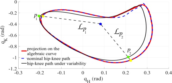
The result of the proposed radial-based projection algorithm for a deviated walking stride onto the human-inspired algebraic curve and its comparison to the normal walking data. The dotted point inside the curve represents the centroid of the algebraic curve. Two example radial lines ${\mathcal{L}}_{p_1}$ and ${\mathcal{L}}_{p_2}$ project points p₁ and p₂ onto the algebraic curve, respectively.

The following proposition states that if the point p belongs to a sufficiently small neighborhood of the algebraic curve, then the radial projection mapping can be efficiently computed using the classical bisection root finding algorithm [38].

Proposition 2. Consider the human-inspired algebraic curve and its centroid. Consider the projection mapping ${\pi }_{\mathcal{Z}(h^{\mathrm{\star }})}(·)$ in Eqs. (43) and (44). In a sufficiently small neighborhood of $\mathcal{Z}(h^{\mathrm{\star }})$, the projection mapping ${\pi }_{\mathcal{Z}(h^{\mathrm{\star }})}(·)$ is well-defined and can be computed via the bisection root finding algorithm.

Proof. Due to the geometry of the level-sets of the IP $h^{\mathrm{\star }}(q_H,q_K)$, the zero set of $h^{\mathrm{\star }}(·)$ is an isolated zero level set. In other words, there exists an open neighborhood of the closed curve $\mathcal{Z}(h^{\mathrm{\star }})$ denoted by $\mathcal{N}$ such that if $q\in \mathcal{N}$ and $h^{\mathrm{\star }}(q)=0$, then $q\in \mathcal{Z}(h^{\mathrm{\star }})$. Consider an arbitrary point $p\in \mathcal{N}$ and suppose that $f_p(0)\ne 0$. Without loss of generality, we assume that $f_p(0)>0$. In other words, p belongs to the exterior of $\mathcal{Z}(h^{\mathrm{\star }})$. Since $\mathcal{Z}(h^{\mathrm{\star }})$ is the only zero set of $h^{\mathrm{\star }}(·)$ in the neighborhood $\mathcal{N}$ and $p\in \mathcal{N}$, it follows that the line ${\ell }_p$ in Eq. (45), which passes through p and the centroid of the closed curve $\mathcal{Z}(h^{\mathrm{\star }})$, intersects the closed curve $\mathcal{Z}(h^{\mathrm{\star }})$ at a unique point $p_0^{*}$. Suppose that $p_0^{*}=p+{\tau }_0^{*}\frac{p-p_{\mathrm{c}}}{\left|\right|p-p_{\mathrm{c}}\left|\right|}$. It follows that $f_p({\tau }_0^{*})=0$. It is now possible to choose a point $p^{\prime }\in \mathcal{N}$ on line ${\ell }_p$, associated with the real number ${\tau }^{-}<0$, in the interior of $\mathcal{Z}(h^{\mathrm{\star }})$ such that $f_p({\tau }^{-})<0$.

Since $f_p(\tau )$ is a smooth function of τ, we have $f_p(0)>0,\hspace{0.17em}{f}_p({\tau }^{-})<0$. Furthermore, ${\tau }_0^{*}$ is the only root of the function $f_p(\tau )$ in the interval $[{\tau }^{-},0]$. From standard results in numerical analysis (see, e.g., Ref. [38]), the proof will be concluded.$\mathrm{■}$

5 Simulation Results

We implemented the impedance-based gait control strategy on an impedance model of the knee dynamics of a human subject. In particular, the impedance modeling of knee dynamics was based on the gait data of a healthy 75 kg subject, as derived from body-mass-normalized data from Winter [30]. Using a variable hip joint motion time profile, generated by the method proposed in Ref. [39], we investigated the effectiveness of our continuous impedance-based scheme and the radial-based projection algorithm in Sec. 4.2. In all of our results, we are working with the algebraic curve shown in Fig. 2(a), which is an improvement over our preliminary work in Ref. [21] shown in Fig. 2(b).

5.1 Algebraic Distances Under Hip-Knee Variability.

In order to study the variations of the generated IP level sets under hip-knee variability during human walking, we generated 100 walking strides using the methodology in Ref. [39]. These profiles are depicted in Fig. 5(a). The values of the IP $h^{\mathrm{\star }}(q_H,q_K)$ on the generated walking data are depicted in Fig. 5(b). As it can be seen from Fig. 5(b), the algebraic distances given by $h^{\mathrm{\star }}(·)$ on the walking strides located at one standard deviation above and below the normal walking data [30] are bounded by the maximum algebraic distance $c_0=4$, which happens during the stance to swing transition (around 60% of the walking stride). As it can be seen from Figs. 2(a) and 5(a), this algebraic distance corresponds to a geometric distance of around 5 deg to the nominal hip-knee configuration. Therefore, the generated IP is not overly sensitive to normal variability in human walking data.

Fig. 5.

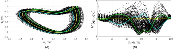
(a) 100 walking strides under hip-knee variability according to Ref. [39] and (b) algebraic distances given by $h^{\mathrm{\star }}(·)$, evaluated on the walking strides. In both figures, the solid curves correspond to one standard deviation above and below the human walking data, respectively.

5.2 Design of Variable Impedance Gains.

In order to design the variable stiffness and damping gains, we have used fourth and third order periodic Bézier polynomials in Eq. (40), respectively. Moreover, periodic variable stiffness gains will be achieved if the equality constraints given by Eq. (41) are satisfied. Furthermore, as implied by Proposition 1, higher values of stiffness to damping ratios, which will result in higher values of $\zeta (\sigma )$, are needed in order to attenuate larger values of the disturbance $\left|\right|d_e(\sigma ,\dot{\sigma })\left|\right|$ along the human-inspired algebraic curve. In order to change the proportional gain $K_p(\sigma )$ continuously along with $\left|\right|d_e(·)\left|\right|$ on the algebraic curve, the coefficients of the stiffness Bézier polynomial are obtained via constrained least-squares optimization to $\left|\frac{d{q}_K^{*}(\sigma )}{d\sigma }\right|$, which is equal to $\frac{\left|\right|d_e(\sigma ,\dot{\sigma })\left|\right|}{\left|\dot{\sigma }\right|}$. Motivated by the observation in Refs. [1] and [6] that the damping gain, during walking, assumes its lower (respectively, larger) values when the proportional gain assumes its larger (respectively, lower) values, the coefficients of the damping Bézier polynomial are obtained via constrained least-squares optimization to $\underset{\sigma }{\max }\frac{d{q}_K^{*}(\sigma )}{d\sigma }-\left|\frac{d{q}_K^{*}(\sigma )}{d\sigma }\right|$. In summary, we find the coefficients of the Bézier polynomials in Eq. (40) by solving the following two constrained optimization problems:

$$\begin{array}{c}\underset{k_{\mathrm{p},i}}{\text{minimize}}{\Vert K_p-\left|\frac{d{q}_{\mathrm{K}}^{*}}{d\sigma }\right|\hspace{0.17em}\Vert }_2^2\\ \text{subject}\hspace{0.17em}\text{to}\hspace{1em}{k}_{\mathrm{p},0}=k_{\mathrm{p},N_{\mathrm{p}}}\end{array}$$

and

$$\begin{array}{c}\underset{k_{\mathrm{d},i}}{\text{minimize}}{\Vert K_d-\left(\underset{\sigma }{\max }\frac{d{q}_{\mathrm{K}}^{*}}{d\sigma }-\left|\frac{d{q}_{\mathrm{K}}^{*}}{d\sigma }\right|\right)\Vert }_2^2\\ \text{subject}\hspace{0.17em}\text{to}\hspace{0.5em}{k}_{\mathrm{d},0}=k_{\mathrm{d},N_{\mathrm{d}}}\end{array}$$

where $\left|\right|·|{|}_2$ denotes the L₂-norm. Moreover, $N_p=4$ and N_d = 2.

Figure 6(a) depicts the normalized variable impedance gains by dividing them by ρ, which is the upper bound on the rate of change of the polar angle (see Eq. (36)), versus the percentage of normal walking stride. The stiffness to damping ratios in our continuous impedance-based scheme are the highest during the stance flexion/extension and swing extension phases of walking and are the lowest during the preswing and swing flexion phases. Interestingly, the stiffness to damping ratios in the conventional switched impedance-based schemes, first proposed in Refs. [1] and [6], also assume their highest and lowest values during the similar phases of walking.

Fig. 6.

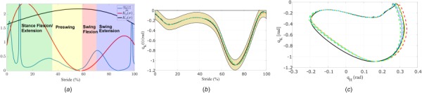
Implementation of the variable impedance-based scheme for five walking strides deviated from Winter's normal motion profile under human hip joint variability: (a) depicts the normalized values of optimized $K_p(\sigma )$ in N·m/deg and $K_d(\sigma )$ in N·ms/deg during a walking stride, (b) depicts the knee time-profiles and their comparison to the normal walking profile (the black curve), and (c) depicts the resulting traversed paths in the hip-knee plane

5.3 Implementation of the Variable Impedance-Based Scheme.

The block diagram of the overall scheme is depicted in Fig. 7. The projection mapping given by Eqs. (43)–(45) provides the variable impedance-based controller with the reference signal $q_K^{*}$ and the polar angle σ. In turn, the variable impedance controller, whose stiffness and damping gains are given by Eq. (40), drives the error $q_K-q_K^{*}(\sigma )$ toward zero, and by doing so, drives the algebraic curve distances to zero.

Fig. 7.

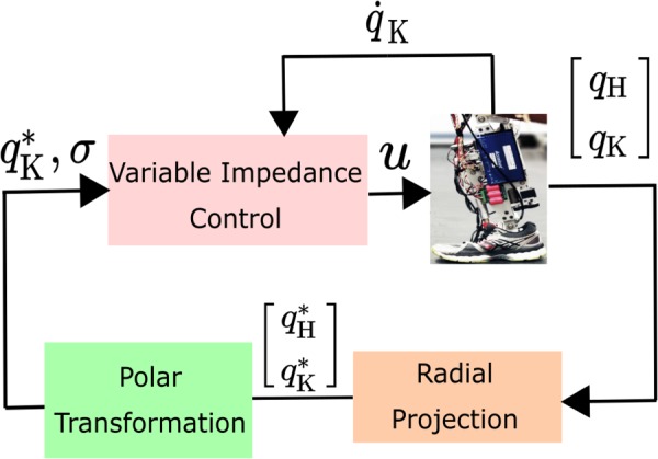
The block diagram of the proposed variable impedance-based scheme. The projection mapping given by Eqs. (43)–(45) provides the variable impedance-based controller given by Eqs.(32) and (40) with the proper reference point on the algebraic curve.

We tested our variable impedance-based scheme for five walking strides deviated from the Winter's normal motion profile under human hip joint variability. Figure 6(b) depicts the knee time-profiles and their comparison to the normal walking profile (the black curve). Figure 6(c) depicts the resulting traversed paths in the hip-knee plane.

6 Conclusions and Future Research Directions

In this article, we employed algebraic curves to represent human walking gait data and achieve coordinated motion between transfemoral amputee patients and powered prosthetic joints. For an impedance model of the knee joint motion driven by the hip angle signal, we proposed using a variable impedance scheme for creating a continuum of equilibria along the human-inspired algebraic curve. Our variable impedance-based control law, which is designed using the parameter-dependent Lyapunov function framework, realized the coordinated hip-knee motion with a family of spring and damper behaviors that continuously change along the human-inspired algebraic curve. Exploiting the geometrical structure of the level-sets of the human-inspired algebraic curve, we proposed a computationally efficient radial projection-based algorithm onto the algebraic curve in the hip-knee plane. We employed the radial projection-based algorithm to accommodate the variability in the human's hip motion in our variable impedance-based scheme. The presented material opens up some potential research directions.

From a theoretical perspective, the 3 L fitting algorithm or its extensions might be employed for fitting trivariate (of three variables) implicit polynomials to hip-knee-ankle human walking data. Moreover, the variable impedance-based scheme needs to consider the nonlinear dynamics of a powered knee-ankle prosthesis and use a proper projection algorithm in order to take into account the variability in human hip motion.

From a control system implementation perspective, the proposed methodology has the potential to be employed for nonrhythmic motions and thus overcome the limitations of existing unified gait control methods for powered prostheses. As the proposed radial projection algorithm can be implemented using a bisection root finding numerical method, it has the potential to be efficiently implemented on an embedded system in real time. Finally, we can fit the algebraic curve, using the same 3 L numerical algorithm, to a global hip measurement for implementation with an inertial measurement unit.

Funding Data

• National Institute of Child Health and Human Development (Grant Nos.: DP2HD080349 and R01HD094772; Funder ID: 10.13039/100000071).

• Burroughs Wellcome Fund (Funder ID: 10.13039/100000861).

References

- [1]. Sup, F. , Bohara, A. , and Goldfarb, M. , 2008, “ Design and Control of a Powered Transfemoral Prosthesis,” Int. J. Robot. Res., 27(2), pp. 263–273. 10.1177/0278364907084588 [DOI] [PMC free article] [PubMed] [Google Scholar]
- [2]. Liu, M. , Zhang, F. , Datseris, P. , and Huang, H. H. , 2014, “ Improving Finite State Impedance Control of Active-Transfemoral Prosthesis Using Dempster-Shafer Based State Transition Rules,” J. Intell. Robot. Syst., 76(3–4), pp. 461–474. 10.1007/s10846-013-9979-3 [DOI] [Google Scholar]
- [3]. Zhang, F. , Liu, M. , and Huang, H. , 2015, “ Investigation of Timing to Switch Control Mode in Powered Knee Prostheses During Task Transitions,” PLoS One, 10(7), p. e0133965. 10.1371/journal.pone.0133965 [DOI] [PMC free article] [PubMed] [Google Scholar]
- [4]. Zhang, F. , Liu, M. , and Huang, H. , 2015, “ Effects of Locomotion Mode Recognition Errors on Volitional Control of Powered Above-Knee Prostheses,” IEEE Trans. Neural Syst. Rehabil. Eng., 23(1), pp. 64–72. 10.1109/TNSRE.2014.2327230 [DOI] [PubMed] [Google Scholar]
- [5]. Simon, A. M. , Ingraham, K. A. , Fey, N. P. , Finucane, S. B. , Lipschutz, R. D. , Young, A. J. , and Hargrove, L. J. , 2014, “ Configuring a Powered Knee and Ankle Prosthesis for Transfemoral Amputees Within Five Specific Ambulation Modes,” PLoS One, 9(6), p. e99387. 10.1371/journal.pone.0099387 [DOI] [PMC free article] [PubMed] [Google Scholar]
- [6]. Fite, K. , Mitchell, J. , Sup, F. , and Goldfarb, M. , 2007, “ Design and Control of an Electrically Powered Knee Prosthesis,” IEEE Tenth International Conference on Rehabilitation Robotics (ICORR), Noordwijk, The Netherlands, June 13–15, pp. 902–905. 10.1109/ICORR.2007.4428531 [DOI] [Google Scholar]
- [7]. Huang, H. , Crouch, D. L. , Liu, M. , Sawicki, G. S. , and Wang, D. , 2016, “ A Cyber Expert System for Auto-Tuning Powered Prosthesis Impedance Control Parameters,” Annals Biomed. Eng., 44(5), pp. 1613–1624. 10.1007/s10439-015-1464-7 [DOI] [PubMed] [Google Scholar]
- [8]. Wen, Y. , Liu, M. , Si, J. , and Huang, H. H. , 2016, “ Adaptive Control of Powered Transfemoral Prostheses Based on Adaptive Dynamic Programming,” IEEE 38th Annual International Conference Engineering Medicine Biology Society (EMBC), Orlando, FL, Aug. 16–20, pp. 5071–5074. 10.1109/EMBC.2016.7591867 [DOI] [PubMed] [Google Scholar]
- [9]. Gregg, R. D. , Lenzi, T. , Hargrove, L. J. , and Sensinger, J. W. , 2014, “ Virtual Constraint Control of a Powered Prosthetic Leg: From Simulation to Experiments With Transfemoral Amputees,” IEEE Trans. Robot., 30(6), pp. 1455–1471. 10.1109/TRO.2014.2361937 [DOI] [PMC free article] [PubMed] [Google Scholar]
- [10]. Villarreal, D. J. , Poonawala, H. A. , and Gregg, R. D. , 2017, “ A Robust Parameterization of Human Gait Patterns Across Phase-Shifting Perturbations,” IEEE Trans. Neural Syst. Rehabil. Eng., 25(3), pp. 265–278. 10.1109/TNSRE.2016.2569019 [DOI] [PMC free article] [PubMed] [Google Scholar]
- [11]. Holgate, M. A. , Sugar, T. G. , and Bohler, A. W. , 2009, “ A Novel Control Algorithm for Wearable Robotics Using Phase Plane Invariants,” IEEE International Conference on Robotics and Automation (ROBOT), Kobe, Japan, May 12–17, pp. 3845–3850. 10.1109/ROBOT.2009.5152565 [DOI] [Google Scholar]
- [12]. Quintero, D. , Villarreal, D. J. , Lambert, D. J. , Kapp, S. , and Gregg, R. D. , 2018, “ Continuous-Phase Control of a Powered Knee–Ankle Prosthesis: Amputee Experiments Across Speeds and Inclines,” IEEE Trans. Robot., 34(3), pp. 686–701. 10.1109/TRO.2018.2794536 [DOI] [PMC free article] [PubMed] [Google Scholar]
- [13]. Quintero, D. , Villarreal, D. J. , and Gregg, R. D. , 2016, “ Preliminary Experiments With a Unified Controller for a Powered Knee-Ankle Prosthetic Leg Across Walking Speeds,” IEEE/RSJ International Conference on Intelligent Robots and Systems (IROS), Daejeon, South Korea, Oct. 9–14, pp. 5427–5433. 10.1109/IROS.2016.7759798 [DOI] [PMC free article] [PubMed] [Google Scholar]
- [14]. Shultz, A. H. , and Goldfarb, M. , 2018, “ A Unified Controller for Walking on Even and Uneven Terrain With a Powered Ankle Prosthesis,” IEEE Trans. Neural Syst. Rehabil. Eng., 26(4), pp. 788–797. 10.1109/TNSRE.2018.2810165 [DOI] [PubMed] [Google Scholar]
- [15]. Quintero, D. , Martin, A. E. , and Gregg, R. D. , 2018, “ Toward Unified Control of a Powered Prosthetic Leg: A Simulation Study,” IEEE Trans. Control Syst. Technol., 26(1), pp. 305–312. 10.1109/TCST.2016.2643566 [DOI] [PMC free article] [PubMed] [Google Scholar]
- [16]. Villarreal, D. J. , Quintero, D. , and Gregg, R. D. , 2017, “ Piecewise and Unified Phase Variables in the Control of a Powered Prosthetic Leg,” IEEE International Conference on Rehabilitation Robotics (ICORR), London, UK, July 17–20, pp. 1425–1430. 10.1109/ICORR.2017.8009448 [DOI] [PMC free article] [PubMed] [Google Scholar]
- [17]. Martin, A. E. , and Gregg, R. D. , 2017, “ Stable, Robust Hybrid Zero Dynamics Control of Powered Lower-Limb Prostheses,” IEEE Trans. Autom. Control, 62(8), pp. 3930–3942. 10.1109/TAC.2017.2648040 [DOI] [PMC free article] [PubMed] [Google Scholar]
- [18]. Quintero, D. , Lambert, D. J. , Villarreal, D. J. , and Gregg, R. D. , 2017, “ Real-Time Continuous Gait Phase and Speed Estimation From a Single Sensor,” IEEE Conference on Control Technology and Applications (CCTA), Mauna Lani, HI, Aug. 27–30, pp. 847–852. 10.1109/CCTA.2017.8062565 [DOI] [PMC free article] [PubMed] [Google Scholar]
- [19]. Kumar, S. , Mohammadi, A. , Gans, N. , and Gregg, R. D. , 2017, “ Automatic Tuning of Virtual Constraint-Based Control Algorithms for Powered Knee-Ankle Prostheses,” IEEE Conference on Control Technology and Applications, Mauna Lani, HI, Aug. 27–30, pp. 812–818. 10.1109/CCTA.2017.8062560 [DOI] [PMC free article] [PubMed] [Google Scholar]
- [20]. Blane, M. M. , Lei, Z. , Çivi, H. , and Cooper, D. B. , 2000, “ The 3 L Algorithm for Fitting Implicit Polynomial Curves and Surfaces to Data,” IEEE Trans. Pattern Anal. Mach. Intell., 22(3), pp. 298–313. 10.1109/34.841760 [DOI] [Google Scholar]
- [21]. Mohammadi, A. , and Gregg, R. D. , 2018, “ Human-Inspired Algebraic Curves for Wearable Robot Control,” ASME Paper No. DSCC2018-9061. 10.1115/DSCC2018-9061 [DOI] [PMC free article] [PubMed] [Google Scholar]
- [22]. Martínez, A. , Lawson, B. , and Goldfarb, M. , 2018, “ A Controller for Guiding Leg Movement During Overground Walking With a Lower Limb Exoskeleton,” IEEE Trans. Robot., 34(1), pp. 183–193. 10.1109/TRO.2017.2768035 [DOI] [PubMed] [Google Scholar]
- [23]. Mohammadi, A. , Horn, J. , and Gregg, R. D. , 2017, “ Removing Phase Variables From Biped Robot Parametric Gaits,” IEEE Conference on Control Technology and Applications (CCTA), Mauna Lani, HI, Aug. 27–30, pp. 834–840. 10.1109/CCTA.2017.8062563 [DOI] [PMC free article] [PubMed] [Google Scholar]
- [24]. Silverman, J. H. , 2009, The Arithmetic of Elliptic Curves, Vol. 106, Springer Science and Business Media, Dordrecht, The Netherlands. [Google Scholar]
- [25]. Unel, M. , and Wolovich, W. A. , 2000, “ On the Construction of Complete Sets of Geometric Invariants for Algebraic Curves,” Adv. Appl. Math., 24(1), pp. 65–87. 10.1006/aama.1999.0679 [DOI] [Google Scholar]
- [26]. Winter, D. A. , 1991, Biomechanics and Motor Control of Human Gait: Normal, Elderly and Pathological, 2nd ed., University of Waterloo Press, Waterloo, ON, Canada. [Google Scholar]
- [27]. Lei, Z. , Blane, M. M. , and Cooper, D. B. , 1996, “ 3 L Fitting of Higher Degree Implicit Polynomials,” Third IEEE Workshop Applications Computer Vision (ACV), Sarasota, FL, Dec. 2–4, pp. 148–153. 10.1109/ACV.1996.572044 [DOI] [Google Scholar]
- [28]. Wolovich, W. , Albakri, H. , and Yalcin, H. , 2002, “ The Precise Measurement of Free-Form Surfaces,” ASME J. Manuf. Sci. Eng., 124(2), pp. 326–332. 10.1115/1.1430677 [DOI] [Google Scholar]
- [29]. Wolovich, W. A. , 2001, “ On the Structure of Algebraic Curves and Their Relation to Dynamical Systems,” IFAC Proc., 34(13), pp. 13–19. 10.1016/S1474-6670(17)38961-9 [DOI] [Google Scholar]
- [30]. Winter, D. A. , 2009, Biomechanics and Motor Control of Human Movement, Wiley, New York. [Google Scholar]
- [31]. Rugh, W. J. , and Shamma, J. S. , 2000, “ Research on Gain Scheduling,” Automatica, 36(10), pp. 1401–1425. 10.1016/S0005-1098(00)00058-3 [DOI] [Google Scholar]
- [32]. Teel, A. , and Praly, L. , 1995, “ Tools for Semiglobal Stabilization by Partial State and Output Feedback,” SIAM J. Control Optim., 33(5), pp. 1443–1488. 10.1137/S0363012992241430 [DOI] [Google Scholar]
- [33]. Gahinet, P. , Apkarian, P. , and Chilali, M. , 1996, “ Affine Parameter-Dependent Lyapunov Functions and Real Parametric Uncertainty,” IEEE Trans. Autom. Control, 41(3), pp. 436–442. 10.1109/9.486646 [DOI] [Google Scholar]
- [34]. Khalil, H. K. , 2002, Nonlinear Systems, Prentice Hall, Upper Saddle River, NJ. [Google Scholar]
- [35]. Mohammadi, A. , 2016, “ Virtual Holonomic Constraints for Euler-Lagrange Control Systems,” Ph.D. thesis, University of Toronto, Toronto, ON, Canada. [Google Scholar]
- [36]. Westervelt, E. R. , Chevallereau, C. , Choi, J. H. , Morris, B. , and Grizzle, J. W. , 2007, Feedback Control of Dynamic Bipedal Robot Locomotion, CRC Press, Boca Raton, FL. [Google Scholar]
- [37]. Westervelt, E. R. , Grizzle, J. W. , and Koditschek, D. E. , 2003, “ Hybrid Zero Dynamics of Planar Biped Walkers,” IEEE Trans. Autom. Control, 48(1), pp. 42–56. 10.1109/TAC.2002.806653 [DOI] [Google Scholar]
- [38]. Atkinson, K. E. , 2008, An Introduction to Numerical Analysis, Wiley, New York. [Google Scholar]
- [39]. Martin, A. E. , Villarreal, D. J. , and Gregg, R. D. , 2016, “ Characterizing and Modeling the Joint-Level Variability in Human Walking,” J. Biomech., 49(14), pp. 3298–3305. 10.1016/j.jbiomech.2016.08.015 [DOI] [PMC free article] [PubMed] [Google Scholar]