Abstract
The problem of the asymptotic dynamics of a quarantine/isolation model with time delay is considered, subject to two incidence functions, namely standard incidence and the Holling type II (saturated) incidence function. Rigorous qualitative analysis of the model shows that it exhibits essentially the same (equilibrium) dynamics regardless of which of the two incidence functions is used. In particular, for each of the two incidence functions, the model has a globally asymptotically stable disease-free equilibrium whenever the associated reproduction threshold quantity is less than unity. Further, it has a unique endemic equilibrium when the threshold quantity exceeds unity. For the case with the Holling type II incidence function, it is shown that the unique endemic equilibrium of the model is globally asymptotically stable for a special case. The permanence of the disease is also established for the model with the Holling type II incidence function. Furthermore, it is shown that adding time delay to and/or replacing the standard incidence function with the Holling type II incidence function in the corresponding autonomous quarantine/isolation model with standard incidence (considered in Safi and Gumel (2010) [10]) does not alter the qualitative dynamics of the autonomous system (with respect to the elimination or persistence of the disease). Finally, numerical simulations of the model with standard incidence show that the disease burden decreases with increasing time delay (incubation period). Furthermore, models with time delay seem to be more suitable for modeling the 2003 SARS outbreaks than those without time delay.
Keywords: Isolation, Quarantine, Time delay, Non-linear incidence, Stability, Equilibria
1. Introduction
The aim of this study is to assess the roles of time delay (to model the incubation period of a disease) and the choice of incidence function in the transmission dynamics of a communicable disease in the presence of quarantine (of exposed individuals) and isolation (of individuals with disease symptoms). Quarantine and isolation measures have been widely used, over the decades, to control the spread of diseases such as yellow fever, smallpox, measles, ebola, pandemic influenza, diphtheria, plague, cholera, and, more recently, severe acute respiratory syndrome (SARS) [1], [2], [3], [4], [5], [6], [7], [8], [9]. To achieve the main objective of this study, the autonomous quarantine/isolation presented in [10] will be extended to incorporate time delay and two different incidence functions. The functional forms of the incidence functions to be considered are derived on the basis of the framework described below.
Let and denote the number of susceptible individuals, the number of infectious individuals and the total size of the population at time , respectively. Further, let be the average number of contacts sufficient for transmitting infection (effective contact rate). Then, the force of infection, given by , represents the average number of contacts that a susceptible individual makes with infectious individuals per unit time. If (i.e., the contact rate depends on the total population, ), then the incidence function is called mass action incidence. If (a constant), then the incidence function is called standard incidence [11], [12]. These two functions are widely used in the modeling the transmission dynamics of the human diseases [13], [14]. Another widely used incidence function is the Holling type II incidence function, given by , with , [15], [16], [17], [18]. The non-linear incidence function of type was first introduced by Capasso and Serio [15], in their study of the cholera epidemic in Bari, Italy. The main justification for using such a functional form of the incidence function stems from the fact that the number of effective contacts between infective individuals and susceptible individuals may saturate at high infective levels due to crowding of infective individuals, or due to the preventive measures taken by (and behavioral changes of) the susceptible individuals in response to the severity of the disease [16], [17], [18].
The paper is organized as follows. The model with standard incidence is formulated in Section 2. The existence and global asymptotic stability of its disease-free equilibrium (DFE), as well as the existence of its endemic equilibrium point (EEP), are established in Section 3. The model with the Holling type II incidence function is formulated and analyzed in Section 4. The permanence of the disease is also established for this model.
2. Model formulation: standard incidence
The model to be considered in this study is that for the transmission dynamics of an infectious disease, in the presence of quarantine of exposed individuals and isolation of infected individuals with disease symptoms, and is given by the following delayed system of integro-differential equations:
| (1) |
where denote the populations of susceptible, exposed, infectious, quarantined, hospitalized and recovered individuals at time , respectively.
Thus, the total human population at time , denoted by , is given by
The initial data for the model (1) is given by
| (2) |
where such that for , and denotes the Banach space of continuous functions mapping the interval into , equipped with the uniform norm defined by . Furthermore, it is assumed that (for ).
In (1), the parameter represents the rate of recruitment into the population, and is the effective contact rate. The delay parameter represents the associated incubation period [19] (see Table 1 for a list of some communicable diseases and their respective incubation periods). Exposed individuals are quarantined at a rate . Quarantined and infectious individuals are hospitalized at the rates and , respectively. The parameters and represent the recovery rates of infectious and hospitalized individuals, respectively, while is the natural death rate. Finally, and are the disease-induced death rates for infectious and hospitalized individuals, respectively. A flow diagram of the model (1) is given in Fig. 1, and the associated variables and parameters are described and estimated in Table 2, Table 3 . It should be stated that the parameter values in Table 3 are relevant to the transmission dynamics of SARS [1], [20], [21], [22].
Table 1.
| Disease | Incubation period (days) |
|---|---|
| Chicken pox | 14–16 |
| Ebola | 2–21 |
| Influenza | 1–3 |
| Measles | 9–12 |
| SARS | Up to 10 |
| Smallpox | 7–17 |
Fig. 1.
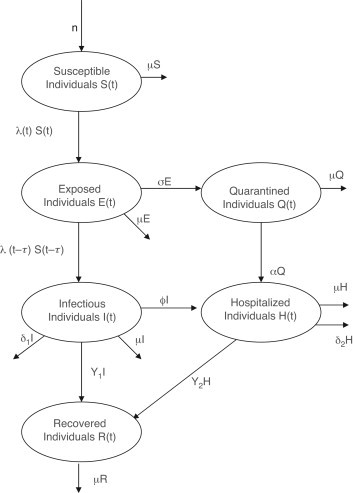
Flow diagram of the delayed model (3).
Table 2.
Description of variables and parameters of the model (3).
| Variable | Description |
|---|---|
| Population of susceptible individuals | |
| Population of exposed individuals | |
| Population of infectious individuals | |
| Population of quarantined individuals | |
| Population of hospitalized individuals | |
| Population of recovered individuals | |
| Parameter | Description |
| Recruitment rate into the community | |
| Natural death rate | |
| Effective contact rate | |
| Incubation period | |
| Parameter for measuring psychological or inhibitory effect | |
| Quarantine rate for exposed individuals | |
| Hospitalization rate for quarantined individuals | |
| Hospitalization rate for infectious individuals | |
| Rate of loss of infection-acquired immunity | |
| Recovery rate for infectious individuals | |
| Recovery rate for hospitalized individuals | |
| Disease-induced death rate for infectious individuals | |
| Disease-induced death rate for hospitalized individuals | |
Table 3.
Estimated values of the parameters of the model (3).
The delayed model (1) is an extension of the autonomous quarantine/isolation model presented in [10] by incorporating a time delay (), but with the assumption of loss of infection-acquired immunity relaxed (i.e., that recovered individuals do not become susceptible again) and the assumption that hospitalized individuals do not transmit infection. One of the main aims of this study is to determine whether or not incorporating time delay (for the incubation period) alters the qualitative dynamics of the autonomous quarantine/isolation model considered in [10]. Another major objective is to determine whether replacing the standard incidence function in the model (1) with the Holling type II incidence function will introduce new (or different) dynamical features for the delayed model (1).
2.1. Basic properties
Using the generalized Leibnitz rule of differentiation [25], the model (1) can be rewritten as a system of delayed differential difference equation given by
| (3) |
The basic qualitative properties of the model (3) will now be investigated.
Lemma 1
The solution of the system (3) , with the initial data (2) , exists for all and is unique. Furthermore, , and for all .
Proof
System (3) can be written as (where a dot represents differentiation with respect to )
where . Since is continuous and Lipschitz in , it follows, by the Fundamental Theory of Functional Differential Equations [26], that the system (3) has a unique solution satisfying the initial data (2).
It is clear from the first equation of the model (3) that
and so
Similarly, it follows from the third equation of the system (3) that for all . Since the second equation of (3) is equivalent to the second equation of (1), it follows (by using the fact that and for all , together with the fact that all the parameters of the model are positive) that
Furthermore, using the same approach as for above, it can be shown that and for all . □
Lemma 2
The closed set
is positively invariant.
Proof
Adding all the equations of the model (3) gives
(4) Since , it follows that if . Thus,
In particular, if . Hence, the region is positively invariant. Further, if , then either the solution enters in finite time, or approaches asymptotically. Hence, the region attracts all solutions in . □
3. Global stability of the DFE
The DFE of the system (3), obtained by setting the derivatives in the model (3) to zero, is given by
| (5) |
The global asymptotic stability property of will be explored using the methodology given in [25], [27]. It is convenient to define
The quantity is known as the basic reproduction number of the delayed model (3). It measures the average number of new infections generated by a single infectious individual in a completely susceptible population. It is worth noting that is a decreasing function of (and for all ).
Theorem 1
The DFE of the model (3) , given by (5) , is GAS in whenever .
Proof
Let . Furthermore, let be any positive solution of the system (3) with the initial data (2). The third equation of the system (3) can be rewritten as
(6) It follows, by using the substitution in (6), that
(7) Taking the of both sides of (7), and noting that [25], gives
(8) Since , it follows that . This is a contradiction, unless . Thus, for any sufficiently small, there exists a such that if , then .
Using and , for , in the second equation of (3) gives
Furthermore, by the comparison theorem [28],
Since is arbitrary, it follows (by setting ) that
Hence, for small, there exists a such that if , then . Using , for , in the fourth equation of (3) gives
and so
Hence,
In a similar way, it can be shown that
Finally, it follows from the first equation of (3), for , that
and so
(9) Hence, by letting in (9),
Additionally, since , it follows that
Thus,
□
This result (Theorem 1) is consistent with that given for the non-delayed quarantine/isolation model in [10] (for the case where recovered individuals do not lose their infection-acquired immunity and hospitalized individuals do not transmit infection for the DFE of the model considered in [10]). That is, this result shows that adding time delay to the non-delayed (autonomous) quarantine/isolation model in [10] does not alter the global asymptomatic stability property of the DFE () of the corresponding non-delayed model given in [10]. The epidemiological implication of Theorem 1 is that the combined use of quarantine and isolation can lead to disease elimination from the community if the two interventions can bring (and keep) the threshold quantity, , to a value less than unity (i.e., for the delayed model (3), the condition is necessary and sufficient for disease elimination).
By solving for the delay parameter () from the equation (and noting Theorem 1), the following result can be obtained.
Lemma 3
The DFE of the model (3) , given by (5) , is GAS in whenever
In other words, Lemma 3 shows that the disease will be eliminated from the community if and only if . Furthermore, it follows from Lemma 3 that the longer infected individuals remain in the exposed class (), the higher the likelihood of disease elimination from the community. Fig. 2 depicts the numerical results obtained by simulating the model (3) using the parameter values in Table 3, and various initial conditions, for the case when . It is evident from this figure that all solutions converged to the DFE, (in line with Theorem 1 and Lemma 3).
Fig. 2.
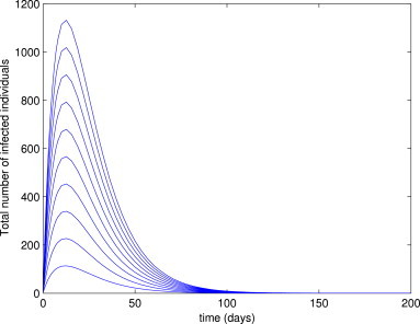
Simulations of the delayed model (3), showing the total number of infected individuals as a function of time. Parameter values used are as given in Table 3, with and (so and ).
3.1. The existence of an EEP
In this section, the possible existence and stability of endemic (positive) equilibria of the model (3) will be explored.
Let represent any arbitrary endemic equilibrium point of the model (3), so . Solving the equations of the model (3) at the steady state gives
| (10) |
where
| (11) |
For computational convenience, the expressions in (10) are rewritten in terms of as below:
| (12) |
where
Substituting the expressions in (12) into (11) gives
| (13) |
Dividing each term in (13) by (and noting that, at the endemic steady state, ) gives
| (14) |
Since
it follows from (14) that
| (15) |
The components of the endemic equilibrium, , can then be obtained by substituting the unique value of , given in (15), into the expressions in (10). Thus, the following result is established.
Lemma 4
The model (3) has a unique endemic (positive) equilibrium, given by , whenever .
Although not proven here, numerical simulations of the model (3) suggest that the EEP () of the model (3) is asymptotically stable for (Fig. 3 ). It should be mentioned, however, that the solutions depicted in Fig. 3 did not converge to zero, as they appear to (see Fig. 4 for a blow up of the tail end of Fig. 3). In other words, Fig. 3, Fig. 4 show convergence of the solutions to the unique EEP, , of the model (3) for the case . The following conjecture is suggested:
Conjecture 1
The unique EEP, , of the model (3) is LAS whenever .
Fig. 3.
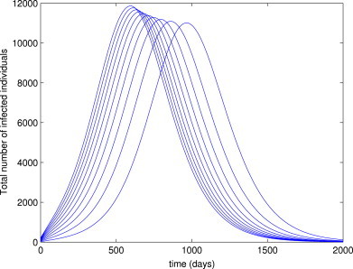
Simulations of the delayed model (3), showing the total number of infected individuals as a function of time. Parameter values used are as given in Table 3, with and (so and ).
Fig. 4.
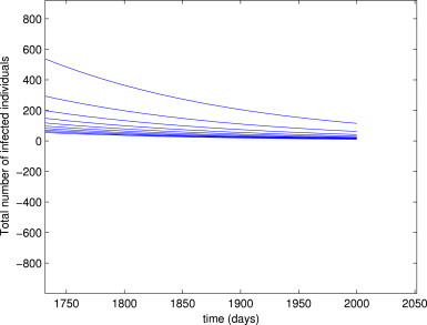
Blow up of the tail end of Fig. 3.
In summary, the model (3) has a globally asymptotic stable disease-free equilibrium whenever , and it has a unique endemic equilibrium whenever . These results are consistent with those reported for the corresponding autonomous (non-delayed) quarantine/isolation model in [10]. In other words, adding time delay to the non-delayed quarantine/isolation model in [10] does not alter its qualitative (equilibrium) dynamics. The next task is to determine whether or not the dynamics of the non-delayed quarantine/isolation model in [10] is affected by the combined use of time delay and the substitution of the standard incidence function with the Holling type II incidence function. This is considered below.
4. The model with Holling type II incidence
In this section, the delayed model (3) will be analyzed subject to the use of the Holling type II incidence function, given by (with ), in place of the standard incidence function. The delayed model (3), with the standard incidence function replaced by , is given by
| (16) |
4.1. Global stability of the DFE
The delayed system (16) has the same DFE, , as the system (3). Further, the invariant region, , holds for system (16) as well. The GAS property of the DFE of the system (16) will be explored using the methodology given in [29]. Define
The proof is based on using the following result.
Lemma 5 [29] —
Consider the following delay differential equation:
(17) where and are positive constants, ; then:
Theorem 2
The DFE of the model (16) , given by (5) , is GAS in whenever .
Proof
Let . Furthermore, let be any positive solution of the system (16) with the initial data (2). Since , it is clear that
(18) Since in for all , it follows from the second equation of (16) that
(19) Consider, next, the auxiliary (with equality) equation associated with the inequality (19) (where is a dummy variable)
(20) Using Item (i) of Lemma 5, together with Eq. (18), in (20) gives
Thus, it follows from (19), using the comparison theorem [28], that
Thus, for any sufficiently small, there exists a such that if , then . Using in and , for , in the second equation of (16) (note that is monotone increasing) gives
Furthermore, by the comparison theorem,
Since is arbitrary, it follows (by setting ) that
Hence, for small, there exists a such that if , then . Using , for , in the fourth equation of (16) gives
and so
Hence,
In a similar way, it can be shown that
Finally, it follows from the first equation of (16), for , that
so, using the comparison theorem,
Hence (by letting )
Additionally, since in it follows that
Thus,
□
The epidemiological implication of the above result (Theorem 2) is that the combined use of quarantine and isolation can lead to disease elimination if the two interventions can bring (and keep) the threshold quantity, , to a value less than unity (i.e., the condition is necessary and sufficient for disease elimination).
By solving for from the equation (and noting Theorem 2), the following result can be obtained.
Lemma 6
The DFE of the model (16) , given by (5) , is GAS in whenever .
In other words, like in the case of system (3), the disease will be eliminated from the community if and only if . Fig. 5 depicts the numerical results obtained by simulating the model (16) using the parameter values in Table 3 and various initial conditions for the case . It is evident from this figure that all solutions converged to the DFE, (in line with Theorem 2 and Lemma 6).
Fig. 5.
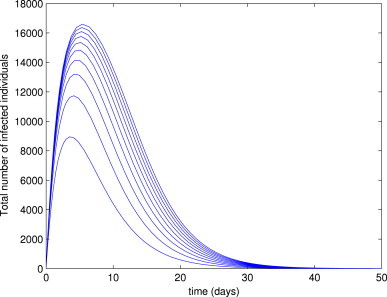
Simulations of the delayed model (16), showing the total number of infected individuals as a function of time. Parameter values used are as given in Table 3, with and (so and ).
4.2. The existence of an EEP and disease permanence
In this section, the possible existence of endemic (positive) equilibria of the model (16), and the permanence of the disease, will be explored.
4.2.1. The existence of an EEP
Let represent any arbitrary endemic equilibrium of the model (16). Solving the equations of the model (16) at the steady state gives
| (21) |
Equating the first and third equations of (21), and solving for in terms , gives
| (22) |
Substituting for from (22) into the first equation of (21) gives
| (23) |
It follows from (21) (noting from (22) and (23) that both and are positive if ) that whenever . Thus, the following result is established.
Lemma 7
The model (16) has a unique endemic (positive) equilibrium, given by , whenever .
4.2.2. Permanence of the disease
The permanence of the disease will now be explored in the context of the model (16). That is, the objective is to determine whether or not the number of infectious cases in the population will persist above a certain positive number for a long time period (for the case when ).
Theorem 3
If , then for any solution of (16) with the initial data (2) , there exists a positive number , such that .
Proof
The proof of Theorem 3 is based on using the approach given in [30], [31], [32], [33]. It should be noted, first of all, that the second equation of (16) can be rewritten as
(24) Consider the following function:
Clearly, is bounded (since the variables and are bounded). Furthermore, it follows, using (24), that
(25) Since, at the endemic steady state, is given by whenever , it is clear that for any , where . Hence, there exists a number such that .
The next task is to show that for all . Suppose, by contradiction, that for all . It then follows, from the first equation of (16), for , that
Hence,
and so, for ,
(26) Since , it follows from (25), for , that
(27) Let . It can be claimed that for all . Suppose the claim does not hold. Then there exists a constant such that for for with and (see Fig. 6 ). However, it follows from the third equation of (16), when , that
This contradicts the fact that . Hence, for . Thus, it follows from (27) that
Hence, , which contradicts the fact that is bounded. Finally, to complete the proof, we need to show that for sufficiently large .
Let be sufficiently large and . Consider the following interval, . It follows, from the second equation of (16), that
Hence,
(28) It is clear from (28) that if , then . For the other case (where ), it is easy to see that the inequity also holds for . We claim that (28) also holds for . If not, then there exists a constant such that for , with for and . Here, too, it follows from the third equation of (16), when , that
This contradicts the fact that . Hence, for . Since this interval and the parameter are chosen arbitrarily, it is concluded that . Thus, . □
Fig. 6.
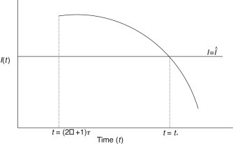
Plot for .
The epidemiological implication of Theorem 3 is that the number of infectious cases will persist in the population (as ) above a certain positive number () whenever .
4.3. Global stability of the EEP
Here, the global stability of the EEP, , of the model (16) will be explored. It is convenient to define
Theorem 4
The unique endemic equilibrium of the model (16) , given by (21) , is GAS in if and .
Proof
The proof of Theorem 4 is based on using a comparison argument and an iteration technique, as given in [29], [34].
Let be any solution of (16) with initial conditions given by (2). Further, let
The goal is to show that
It follows from the first equation of (16) that
and so, by the comparison theorem,
Let . Thus, for sufficiently small , there exists a such that for . It follows from the third equation of (16) that, for ,
(29) Consider the auxiliary equation of (29):
(30) Since , it follows that, for sufficiently small . Hence, by Item (ii) of Lemma 5 and (30),
Thus, by the comparison theorem,
and so
Similarly, let
Then, for sufficiently small , there exists a such that for . It follows from the first equation of (16), for , that
and so, by the comparison theorem,
Hence, , where . In other words, for sufficiently small , there exists a such that for . It follows from the third equation of (16), for , that
and so (by considering the auxiliary equation)
Hence, it follows from Item (ii) of Lemma 5 (since ) that
and the comparison theorem gives
Hence, for sufficiently small , there exists a such that for , where
Using , and in the second equation of (16), for , gives
Hence, by the comparison theorem,
Therefore, for sufficiently small , there exists a such that for , where
Similarly, by using and in the second equation of (16), for , we have
and so
Hence, for sufficiently small , there exists a such that for , where
Using in the fourth equation of (16), for , gives
and so
Thus, for sufficiently small , there exists a such that for , where .
Similarly, by using in the fourth equation of (16), for , we have
and
Thus, for sufficiently small , there exists a such that for , where . Using and in the fifth equation of (16), for , gives
and
Thus, for sufficiently small , there exists a such that , for , where . Similarly, it follows by using and in the fifth equation of (16), for , that
and so
Hence, for sufficiently small , there exists a such that for , where .
Using and in the last equation of (16), for , gives
Hence,
Thus, , where . Using and in the last equation of (16), for , gives
and so (by the comparison theorem)
Hence, , where .
Continuing in this manner leads to the following sequences:
(31) Finally, since , and , the proof is concluded by showing that
Using the first four sequences of (31), it is easy to see that the sequence can be written in terms of as
(32) where . Furthermore, it can be shown that whenever , the sequence is monotone as follows:
Since , it follows that
Thus, exists.
Let . Then, it follows from (32) that
and so
Taking the limit as of both sides of the third sequence of (31) gives
Similarly, taking the limits of both sides of the remaining sequences in (31), and using the previous results, gives
Hence, . □
Theorem 4 shows that the disease will persist in the population whenever . Here, too, by solving for from , the following result can be shown.
Lemma 8
The unique endemic equilibrium of the model (16) , given by (21) , is GAS in if and .
Theorem 4 shows that the disease will persist in the population provided that and . Thus, Lemma 6, Lemma 8 suggest that is a sharp epidemiological threshold that governs the persistence () and elimination () of the disease in the population. Fig. 7 shows a time series plot of the total number of infected individuals for various initial conditions. This figure clearly shows convergence of the solutions to the EEP for the case (in line with Theorem 4 and Lemma 8). Fig. 8 depicts of the total number of cases as a function of time for various values of . This figure shows a decreasing number of cases with increasing values of delay parameter . That is, the longer individuals stay in the exposed class, the lower the disease burden.
Fig. 7.
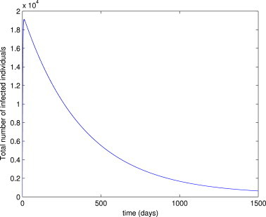
Simulations of the delayed model (16), showing the total number of infected individuals as a function of time. Parameter values used are as given in Table 3, with and (so and ).
Fig. 8.
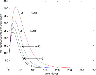
Simulations of the delayed model (16), showing the total number of infected individuals for various values of . Parameter values used are as given in Table 3, with .
To assess the impact of using time delay to model the incubation period on the suitability of the model (3) for realistically capturing the observed SARS data (cumulative probable cases) for the Greater Toronto Area (GTA) of Canada, the model (3) is simulated in the presence and absence of time delay. It should be stated that the GTA recorded about 250 probable cases of SARS during the 2003 outbreaks [21]. The simulation results obtained, depicted in Fig. 9 , show that while the model without time delay (considered in [10]) underestimated the observed cumulative number of probable cases (about 170 cases), the model with time delay (i.e., model (3)) gave a good estimate of the observed data (about 220 cases). Thus, this study suggests that the model (3), with time delay, is more appropriate for modeling the SARS outbreaks in the GTA than the corresponding model without time delay (given in [10]). Similar simulation results were obtained for the case of the model with Holling type II function (16) (see Fig. 10 ).
Fig. 9.
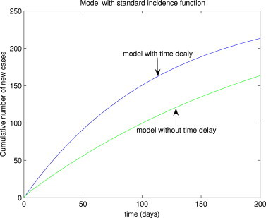
Numerical simulations of the standard incidence delayed model (3), showing the cumulative number of probable SARS cases for the GTA, in the presence and absence of time delay.
Fig. 10.
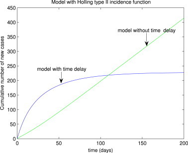
Numerical simulations of the Holling type II delayed model (16), showing the cumulative number of probable SARS cases for the GTA, in the presence and absence of time delay.
5. Conclusions
A deterministic quarantine/isolation model with time delay is considered, subject to two incidence functions, namely standard incidence and the Holling type II incidence function. The main findings of this study are summarized below:
-
(i)
The model with standard incidence function, given by (3), has a globally asymptotically stable disease-free solution whenever a certain epidemiological threshold quantity () is less than unity (Theorem 1). Furthermore, this model has a unique positive endemic equilibrium whenever the threshold quantity () exceeds unity (Lemma 4).
-
(ii)
The model with Holling type II incidence function, given by (16), has a globally asymptotically stable disease-free solution whenever its associated epidemiological threshold quantity () is less than unity (Theorem 2). This model has a unique positive endemic equilibrium whenever the threshold quantity () exceeds unity (Lemma 7). Furthermore, the model system is permanent whenever (Theorem 3). The unique endemic equilibrium of the model (16) is globally asymptotically stable under certain conditions (Theorem 4).
In summary, the theoretical analyses in this study show that adding time delay to and/or replacing the standard incidence function by a Holling type II incidence function in the autonomous (non-delayed) quarantine/isolation model in [10] does not alter the qualitative dynamics (as regards the elimination or persistence of the disease) of the non-delayed model considered in [10]. In other words, the theoretical results in this study show that the quarantine/isolation model with time delay () and standard or non-linear incidence function of Holling type II has essentially the same qualitative (equilibrium) dynamics as the corresponding autonomous quarantine/isolation model () with the standard incidence function considered in [10].
Numerical simulations of the delayed model with the standard incidence function show that the associated disease burden decreases with increasing time delay (). Furthermore, models with time delay seem to be more appropriate for modeling the SARS epidemic than those without time delay (regardless of which of the incidence functions is used).
Acknowledgements
ABG acknowledges, with thanks, the partial support of the Natural Science and Engineering Research Council (NSERC) and Mathematics of Information Technology and Complex Systems (MITACS) of Canada. MAS gratefully acknowledges the support of the University of Manitoba Graduate Fellowship. The authors are grateful to the anonymous reviewers for their constructive comments.
References
- 1.Chowell G., Hengartner N.W., Castillo-Chavez C., Fenimore P.W., Hyman J.M. The basic reproductive number of ebola and the effects of public health measures: the cases of Congo and Uganda. Journal of Theoretical Biology. 2004;1:119–126. doi: 10.1016/j.jtbi.2004.03.006. [DOI] [PubMed] [Google Scholar]
- 2.Hethcote H.W., Ma Zhien, Liao Shengbing. Effects of quarantine in six endemic models for infectious diseases. Mathematical Biosciences. 2002;180:141–160. doi: 10.1016/s0025-5564(02)00111-6. [DOI] [PubMed] [Google Scholar]
- 3.Lipsitch M. Transmission dynamics and control of severe acute respiratory syndrome. Science. 2003;300:1966–1970. doi: 10.1126/science.1086616. [DOI] [PMC free article] [PubMed] [Google Scholar]
- 4.Lloyd-Smith J.O., Galvani A.P., Getz W.M. Curtailing transmission of severe acute respiratory syndrome within a community and its hospital. Proceedings of the Royal Society of London, Series B. 2003;170:1979–1989. doi: 10.1098/rspb.2003.2481. [DOI] [PMC free article] [PubMed] [Google Scholar]
- 5.McLeod R.G., Brewster J.F., Gumel A.B., Slonowsky D.A. Sensitivity and uncertainty analyses for a SARS model with time-varying inputs and outputs. Mathematical Biosciences and Engineering. 2006;3:527–544. doi: 10.3934/mbe.2006.3.527. [DOI] [PubMed] [Google Scholar]
- 6.Riley S. Transmission dynamics of etiological agent of SARS in Hong Kong: the impact of public health interventions. Science. 2003;300:1961–1966. doi: 10.1126/science.1086478. [DOI] [PubMed] [Google Scholar]
- 7.Wang W., Ruan S. Simulating the SARS outbreak in Beijing with limited data. Journal of Theoretical Biology. 2004;227:369–379. doi: 10.1016/j.jtbi.2003.11.014. [DOI] [PMC free article] [PubMed] [Google Scholar]
- 8.Webb G.F., Blaser M.J., Zhu H., Ardal S., Wu J. Critical role of nosocomial transmission in the Toronto SARS outbreak. Mathematical Biosciences and Engineering. 2004;1:1–13. doi: 10.3934/mbe.2004.1.1. [DOI] [PubMed] [Google Scholar]
- 9.Yan X., Zou Y. Optimal and sub-optimal quarantine and isolation control in SARS epidemics. Mathematical and Computer Modelling. 2008;47:235–245. doi: 10.1016/j.mcm.2007.04.003. [DOI] [PMC free article] [PubMed] [Google Scholar]
- 10.Safi M.A., Gumel A.B. Global asymptotic dynamics of a model for quarantine and isolation. Discrete and Continuous Dynamical Systems. Series B. 2010;14:209–231. [Google Scholar]
- 11.Hethcote H.W. The mathematics of infectious diseases. SIAM Review. 2000;42:599–653. [Google Scholar]
- 12.Sharomi O. Role of incidence function in vaccine-induced backward bifurcation in some HIV models. Mathematical Biosciences. 2007;210:436–463. doi: 10.1016/j.mbs.2007.05.012. [DOI] [PubMed] [Google Scholar]
- 13.Anderson R.M., May R.M. Springer-Verlag; Berlin, Heidelberg, New York: 1982. Population Biology of Infectious Diseases. [Google Scholar]
- 14.R.M. Anderson, R.M. May, Infectious Diseases of Humans: Dynamics and Control, Oxford University, London, New York, 1991.
- 15.Capasso V., Serio G. A generalization of the Kermack–McKendrick deterministic epidemic model. Mathematical Biosciences. 1978;42:43–61. [Google Scholar]
- 16.Hou J., Teng Z. Continuous and impulsive vaccination of SEIR epidemic models with saturation incidence rates. Mathematics and Computers in Simulation. 2009;79:3038–3054. [Google Scholar]
- 17.Liu W., Levin S., Iwasa Y. Influence of nonlinear incidence rates upon the behavior of SIRS epidemiological models. Journal of Mathematical Biology. 1986;23:187–204. doi: 10.1007/BF00276956. [DOI] [PubMed] [Google Scholar]
- 18.Ruan S., Wang W. Dynamical behavior of an epidemic model with a nonlinear incidence rate. Journal of Differential Equations. 2003;188:135–163. [Google Scholar]
- 19.Cooke K.L., van den Driessche P. Analysis of an SEIRS epidemic model with two delays. Journal of Mathematical Biology. 1996;35:240–260. doi: 10.1007/s002850050051. [DOI] [PubMed] [Google Scholar]
- 20.Donnelly C. Epidemiological determinants of spread of a causal agent of severe acute respiratory syndrome in Hong Kong. Lancet. 2003;361:1761–1766. doi: 10.1016/S0140-6736(03)13410-1. [DOI] [PMC free article] [PubMed] [Google Scholar]
- 21.Gumel A.B. Modelling strategies for controlling SARS outbreaks. Proceedings of the Royal Society of London, Series B. 2004;271:2223–2232. doi: 10.1098/rspb.2004.2800. [DOI] [PMC free article] [PubMed] [Google Scholar]
- 22.Leung G. The epidemiology of severe acute respiratory syndrome in the 2003 Hong Kong epidemic: an analysis of all 1755 patients. Annals of Internal Medicine. 2004;9:662–673. doi: 10.7326/0003-4819-141-9-200411020-00006. [DOI] [PubMed] [Google Scholar]
- 23.Wikipedia, Incubation Period. www.en.wikipedia.org (accessed May 2010).
- 24.Chowell G., Castillo-Chavez C., Fenimore P.W., Kribs-Zaleta C.M., Arriola L., Hyman J.M. Model parameters and outbreak control for SARS. EID. 2004;10:1258–1263. doi: 10.3201/eid1007.030647. [DOI] [PMC free article] [PubMed] [Google Scholar]
- 25.Kribs-Zaleta C., Velasco-Hernandez J. A simple vaccination model with multiple endemic states. Mathematical Biosciences. 2000;164:183–201. doi: 10.1016/s0025-5564(00)00003-1. [DOI] [PubMed] [Google Scholar]
- 26.Hale J. Springer-Verlag; Heidelberg: 1977. Theory of Functional Differential Equations. [Google Scholar]
- 27.Mukandavire Z., Chiyaka C., Garira W., Musuka G. Mathematical analysis of a sex-structured HIV/AIDS model with a discrete time delay. Nonlinear Analysis. 2009;71:1082–1093. [Google Scholar]
- 28.Smith H.L., Waltman P. Cambridge University Press; 1995. The Theory of the Chemostat. [Google Scholar]
- 29.Xu R., Ma Z. Global stability of a SIR epidemic model with nonlinear incidence rate and time delay. Nonlinear Analysis: Real World Applications. 2009;10:3175–3189. [Google Scholar]
- 30.Gao Shujing, Chenc Lansun, Teng Zhidong. Pulse vaccination of an SEIR epidemic model with time delay. Nonlinear Analysis: Real World Applications. 2008;9:599–607. [Google Scholar]
- 31.Ma W., Song M., Takeuchi Y. Global stability of an SIR epidemic model with time delay. Applied Mathematics Letters. 2004;17:1141–1145. [Google Scholar]
- 32.Wang W. Global behavior of an SEIRS epidemic model with time delays. Applied Mathematics Letters. 2002;15:423–428. [Google Scholar]
- 33.Zhang T., Teng Z. Extinction and permanence for a pulse vaccination delayed SEIRS epidemic model. Chaos, Solitons and Fractals. 2009;39:2411–2425. [Google Scholar]
- 34.Xu R., Ma Z. Stability of a delayed SIRS epidemic model with a nonlinear incidence rate. Chaos, Solitons and Fractals. 2009;41:2319–2325. [Google Scholar]


