Pattern transitions in spatial epidemics: Mechanisms and emergent properties

Abstract

Infectious diseases are a threat to human health and a hindrance to societal development. Consequently, the spread of diseases in both time and space has been widely studied, revealing the different types of spatial patterns. Transitions between patterns are an emergent property in spatial epidemics that can serve as a potential trend indicator of disease spread. Despite the usefulness of such an indicator, attempts to systematize the topic of pattern transitions have been few and far between. We present a mini-review on pattern transitions in spatial epidemics, describing the types of transitions and their underlying mechanisms. We show that pattern transitions relate to the complexity of spatial epidemics by, for example, being accompanied with phenomena such as coherence resonance and cyclic evolution. The results presented herein provide valuable insights into disease prevention and control, and may even be applicable outside epidemiology, including other branches of medical science, ecology, quantitative finance, and elsewhere.

Highlights

• •Transitions between patterns are emergent properties in spatial epidemics.
• •Two types of pattern transitions in infectious diseases are shown.
• •We provide possible mechanisms of pattern transition in spatial epidemics.
• •Pattern transition promotes complexity in spatial epidemics.
• •The results are applicable in medical science, ecology, quantitative finance and so on.

1. Introduction

Despite advances in their prevention and control, infectious diseases are still a threat to human health. In 2009, for example, influenza A(H1N1) outbroke in Mexico and spread throughout the world, ultimately reaching 214 countries and regions, and resulting in about 18,500 deaths [1]. In 2013, a new type of avian influenza, H7N9, appeared in Mainland China and subsequently caused considerable economic losses alongside public health risks [2]. In 2014, Ebola virus disease emerged in West Africa and infected more than 10,000 people [3], [4]. Another new virus—Middle East Respiratory Syndrome coronavirus (MERS-CoV)—had emerged in 2012 and by mid 2015 caused 1,379 human infections with a death toll of 531 people from 26 countries [5]. A particularly instructive case of MERS-CoV outbreak happened in South Korea where 164 infections and 23 deaths were traced back to an individual traveling from the Middle East. These examples illustrate the dangers associated with infectious diseases and the origins of motivation for modeling their transmission dynamics.

Mathematical models have a long tradition in epidemiology and represent a useful tool for revealing the transmission dynamics of infectious diseases. Starting in 1760, Bernoulli was the first to investigate the effectiveness of smallpox vaccination by means of mathematical techniques [6]. In 1906, Hamer resorted to the law of mass action to find the causes of the repeated outbreaks of measles [7]. In 1911, a Nobel Prize winner Ronald Ross used a differential equation to describe the transmission of malaria between humans and mosquitoes [8]. In 1927, Kermack and McKendrick put forth a mathematical framework for compartmental models in epidemiology [9] that has been in use ever since. At about the same time, Reed and Frost developed a chain binomial model with the recognizable susceptible–infectious–recovered (SIR) structure, but their work remained unpublished until exposed by others [10].

If only temporal (as opposed to spatial) dynamics is considered, the basic reproduction number—defined as “the average number of secondary cases caused by an infectious individual in a completely susceptible population” [11]—is the key quantity for determining the fate of epidemics. When this number is less than unity, a pathogen goes extinct regardless of the initial conditions; otherwise, the pathogen persists and the number of infections increases through time [11], [12], [13], [14], [15]. Although studies on the temporal dynamics of diseases proved insightful, observations that pathogens (like substances) diffuse from high to low density regions of space enticed the development of spatially explicit models capable of discerning, for example, disease transmission hotspots. Incorporating space explicitly into epidemiological models revealed that a pathogen may go extinct even if the basic reproduction number is greater than unity [16]. Spatial dynamics occasionally induced chaos [17] and displayed various emergent properties [18]. The overwhelming conclusion was that the role of space in epidemic spread is non-negligible and therefore warrants further study of spatial dynamics in the context of disease transmission.

Spatially explicit models in epidemiology display two properties of interest: traveling wave solutions [19], [20], [21], [22] and pattern formation [23], [24], [25], [26], [27], [28]. Traveling waves characterize the transition between the different equilibrium states, whereas pattern formation is representative of the distribution of individuals in both time and space. Because we are interested primarily in the distribution and the transmission of infectious diseases in space, this review focuses on spatial patterns, the underlying mechanisms, and related emergent properties.

1.1. Epidemiological models without spatial dynamics

A population with an active pathogenic agent is often divided into three compartments. Healthy individuals are susceptible to an infection (S), infectious individuals carry and transmit the pathogen regardless of whether they exhibit symptoms (I), and recovered individuals remain unaffected by the disease (R). These recovered individuals are assumed to either have natural immunity or immunity attained by recuperating from the infection [11], [12], [13]. Sometimes individuals lost to the disease are mixed with those who have recovered in which case R stands for removed. Based on the described compartmentalization, the classical Susceptible–Infectious–Removed (SIR) model without spatial dynamics has the following form:

$$\begin{array}{cc}\hfill & \frac{dS}{dt}=-\beta SI,\hfill \\ \hfill & \frac{dI}{dt}=\beta SI-\gamma I,\hfill \\ \hfill & \frac{dR}{dt}=\gamma I,\hfill \end{array}$$ (1)

where β and γ are infection and recovery (removal) rates, respectively. The basic reproductive number of system (1) is $R_0=\beta S_0/\gamma$, where $S_0$ is the initial number of susceptible individuals. If $R_0<1$, the number of infectious individuals is a decreasing function of time and the disease disappears after a while; otherwise, the disease eventually outbreaks.

1.2. Spatial dynamics in epidemiology by means of reaction–diffusion equations and cellular automata

Reaction–diffusion equations and cellular automata are the common mathematical tools in the studies on the spatially explicit transmission dynamics of infectious diseases. The former tool implies that space is a continuum of points in which the movement of individuals is random. Reaction–diffusion equations are applicable to environments of almost any size and shape, account for the typical rates of motion through space, and reveal the consequent temporal and spatial formation and variation of the distribution of individuals. A reaction–diffusion-based Susceptible–Infected–Susceptible (SIS) model is given by the following equations:

$$\begin{array}{cc}\hfill & \frac{\partial S}{\partial t}=F(S,I)+D_1{\mathrm{\nabla }}^{2}S,\hfill \\ \hfill & \frac{\partial I}{\partial t}=G(S,I)+D_2{\mathrm{\nabla }}^{2}I,\hfill \end{array}$$ (2)

where $F(S,I)$ and $G(S,I)$ are reaction terms describing interactions between the different individuals, and ${\mathrm{\nabla }}^{2}S$ and ${\mathrm{\nabla }}^{2}I$ are diffusion terms representing the spatial motion of susceptible and infectious individuals, respectively (a derivation of ${\mathrm{\nabla }}^2$ is found in Appendix A.1).

Unlike reaction–diffusion equations, the representation of a dynamical system by means of cellular automata is discrete in space, time, and state. The evolution of the system is dependent on the state of a cell and the interactions between cells. More precisely, if cellular automata are to be used in modeling the transmission dynamics of infectious diseases, five elements are essential: (i) a lattice determining the arrangement of cells along with the definition of a cell's neighborhood, (ii) initial and boundary conditions, (iii) the classification of possible states, (iv) disease transmission rules, and (v) parameter values. A simple example of how cellular automata represent the spread of a disease is shown in Fig. 1 . In this example, two events occur simultaneously; infection, whereby the state of a cell changes from susceptible to infectious and recovery, whereby the state of a cell changes from infectious to susceptible. With cellular automata, it is relatively straightforward to enrich the transmission dynamics of infectious diseases with a number of different phenomena like birth, death, migration, etc. [29], [30], [31].

Fig. 1.

Representation of epidemics in a 2-D regular lattice using cellular automata. (a) von Neumann (left) and Moore (right) neighborhoods. (b) An infectious neighbor infects a susceptible individual at a rate β, whereas an infectious individual turns susceptible on its own at a rate γ. (c) The same as (b) except that an infectious individuals recovers permanently on its own.

1.2.1. An example of a hantavirus epidemics model based on reaction–diffusion equations

Hantaviruses of Bunyaviridae family are usually carried by rodents and may infect humans through exposure to saliva, urine, or feces [32], [33]. We consider the transmission dynamics of hantaviruses within a rodent population. This population contains M individuals divided into two classes, susceptible and infectious with $M_S$ and $M_I$ individuals, respectively. Transmission dynamics of hantaviruses in a rodent population is determined by four main factors which include births, deaths, competition, and infections [28], [34], [35], [36].

• Births. All individuals reproduce with birth rate b, implying that the number of newborns per unit of time is $bM=b(M_S+M_I)$. Newborns are treated as being susceptible.

• Deaths. Susceptible and infectious individuals die with mortality rates $c_S$ and $c_I$, respectively. The number of deaths per unit of time is thus $c_S{M}_S+c_I{M}_I$.

• Competition. Due to limited resources, individuals compete with each other. This competition gives rise to the concept of carrying capacity, K, which acts to suppress the population growth as M approaches K. Accordingly, competition causes an additional number of deaths given by the term $M_{S}M/K$ and $M_{I}M/K$ for susceptible and infectious individuals, respectively.

• Infections. An infection is possible if a susceptible and an infectious individual meet and stay in contact for the sufficient amount of time. This possibility is reflected in the contact and transmission rate, β, which gives the probability of an infection per unit of time spent in contact. The probability of meeting an infectious individual is simply given by the fraction of such individuals in the whole population, i.e. $M_I/M$. The number of new infections is therefore $\beta M_S{M}_I/M$. An implicit assumption in the last expression, called the standard incidence rate, is that one susceptible individual meets only one other individual per unit of time who may be infectious with the probability $M_I/M$ and susceptible with the remaining probability $1-M_I/M$. However, one readily envisions a situation in which a large population allows a susceptible individual to make several contacts per unit of time. To account for this possibility, the so-called contact frequency, $C(M)$, can be introduced as a function of the population size. Two functional forms are found in the literature [11], [12], [13]. First, $C(M)=\gamma M$ leads to an interaction term of the form ${\beta }^{\prime }{M}_S{M}_I$ (where ${\beta }^{\prime }=\beta \gamma$ is a new parameter) called the bilinear incidence rate. In this case, the larger the population, the more contacts a susceptible individual makes. Second, $C(M)=M/(\gamma +\delta M)$ results in the infection term ${\beta }^{\prime }{M}_S{M}_I/(1+{\delta }^{\prime }M)$ (where ${\beta }^{\prime }=\beta /\gamma$ and ${\delta }^{\prime }=\delta /\gamma$ are constants) named the saturated incidence rate. This rate is similar to the bilinear incidence rate if the population is small, but mimics the standard incidence rate (with parameter $\beta ={\beta }^{\prime }/{\delta }^{\prime }$) when the population becomes large.

The considerations so far and the corresponding transmission flow in Fig. 2 yield the following hantavirus infection model based on reaction–diffusion equations:

$$\begin{array}{cc}\hfill & \frac{\partial M_S}{\partial t}=b(M_S+M_I)-c_S{M}_S-M_S\frac{M}{K}-\beta C(M)M_S\frac{M_I}{M}+D{\mathrm{\nabla }}^2{M}_S,\hfill \\ \hfill & \frac{\partial M_I}{\partial t}=-c_I{M}_I-M_I\frac{M}{K}+\beta C(M)M_S\frac{M_I}{M}+D{\mathrm{\nabla }}^2{M}_I.\hfill \end{array}$$ (3)

The total population size obeys the standard Fisher equation [37] obtained here by summing the above reaction–diffusion equations and assuming $c_S=c_I=c$:

$$\frac{\partial M}{\partial t}=bM-cM-\frac{M^2}{K}+D{\mathrm{\nabla }}^{2}M.$$ (4)

Fig. 2.

The transmission flow diagram of hantavirus epidemics in a rodent population. Biological interpretation of the parameters is given in the text.

1.3. Pattern formation and spatial dynamics in epidemiology

Spatial patterns characterize the spread of diseases in a manner that may predict transmission dynamics in space. For example, spatial patterns are indicative of the large scale trends of epidemics or of the rates of spread through space, which in turn may guide policy decisions. The types of patterns found in epidemiological studies include stationary patterns [38], [39], [40], [41], [42], wave patterns [43], [44], [45], [46], [47], patch invasion [48], and others [49], [50], [51], [52].

Pattern formation is more than just a theoretical concept. Spatial patterns have been observed empirically, thus confirming the practical value of modeling the transmission dynamics of diseases in space. For example, Grassly et al. [39] showed evidence of pattern formation in the case of poliovirus in India between 2000 and 2005. The results identified a “hot area” for poliovirus (see Fig. 3 (a)) and, more importantly, helped explain the underlying causes of such a phenomenon. Another good example [53] is the predicted distribution of hantavirus pulmonary syndrome in southwestern USA during the 1990s (see Fig. 3(b)). In this case, the results indicated a transition between stationary patterns due to the changes in local environmental conditions.

Fig. 3.

Spatial patterns and empirical evidence. (a) The distribution of poliovirus in India indicating a “hot area” of the virus persistence towards the north. The figure is reproduced from [39]. (b) Location of hantavirus pulmonary syndrome in southwestern USA with risk represented on an arbitrary scale from low (dark blue) to medium (yellow) to high (red). The figure is reproduced from [53]. (For interpretation of the references to color in this figure legend, the reader is referred to the web version of this article.)

1.4. Organization of this review

Although pattern formation and the accompanying transitions have received considerable attention in spatial epidemiology, these phenomena are far from being fully understood. In particular, the underlying causes of pattern transitions and the role these transitions play in the spread of diseases have only recently become a major concern for epidemiological studies. We therefore systematically review the topic of pattern transitions in spatial epidemiology focusing mainly on the following three aspects: (i) the emergence and types of pattern transitions, (ii) the mechanisms causing pattern transitions, and (iii) the epidemiological role of pattern transitions.

The rest of this review is organized as follows. In Section 2, we present the two contrasting types of pattern transitions. First are the transitions between stationary spatial patterns. Second are the transitions between spatio-temporal patterns. Section 3 covers the underlying mechanisms of pattern transitions. In Section 4, we show the three major ways of how pattern transitions contribute to the complexity in spatial epidemics. In the final section, we draw the main conclusions and discuss the potential for future developments.

2. Emergence and types of pattern transitions

Among the main concerns in relation to the spread of infectious diseases are the identification of transmission modalities and the effectiveness of control strategies [54], [55], [56]. Models considering spatial dynamics reveal the consequences of the former issue and suggest new approaches to the latter one. Specifically, a given transmission modality may lead to a recognizable spatial pattern, which then may serve as a basis for planning a control strategy. In this context, two main types of spatial patterns are often mentioned in the literature. Stationary patterns remain unchanged in time and often exhibit intermittent areas of high density of infectious individuals that may favor the persistence of diseases [38], [39], [40]. By contrast, spatio-temporal patterns change over time, either as (i) quasi-periodic or oscillatory waves, (ii) temporal or spatio-temporal chaos, or even (iii) turbulence [57], [58], [59], [60], [61], [62], [63]. In accordance with the two types of spatial patterns, we are interested in two types of transitions. These two types are transitions between stationary patterns, on the one hand, and spatio-temporal patterns, on the other hand.

2.1. Transitions between stationary patterns

The spread of diseases among humans may persist in a stable state (endemic) such that the densities of susceptible, infectious, and/or recovered individuals form striking, self-organized spatial patterns [53], [64]. We proceed to construct two epidemic models, one based on the reaction–diffusion (R-D) equation and the other on cellular automata (CA), to illustrate the emergence of transition between the different types of stationary patterns.

We assume that a population is comprised of three types of individuals. Healthy individuals are susceptible to an infection (S), infectious individuals carry and transmit the disease although they may not exhibit the symptoms yet (I), and removed individuals neither contract nor transmit the disease (R) because they may have natural immunity, may be immune after a recovery, or may have been placed in isolation [11], [12], [65]. Having introduced these three types, we can construct an SIR reaction–diffusion model in the spirit of Eqs. (2) as follows [42]:

$$\begin{array}{cc}\hfill & \frac{\partial S}{\partial t}=A-dS-\beta S^p{I}^q+D_1{\mathrm{\nabla }}^{2}S,\hfill \\ \hfill & \frac{\partial I}{\partial t}=\beta S^p{I}^q-(d+\mu +\gamma )I+D_2{\mathrm{\nabla }}^{2}I,\hfill \\ \hfill & \frac{\partial R}{\partial t}=\gamma I-dR+D_3{\mathrm{\nabla }}^{2}R,\hfill \end{array}$$ (5)

where A is the population's recruitment rate, d is the natural mortality rate, μ is the disease-related mortality rate of infectious individuals, and γ is their recovery rate. The nonlinear incidence rate, $\beta S^p{I}^q$, is due to saturation or multiple exposures before an infection occurs, where p and q are phenomenological constants [66], [67]. ${\mathrm{\nabla }}^2=\frac{{\partial }^2}{\partial X^2}+\frac{{\partial }^2}{\partial Y^2}$ is the usual Laplacian operator in two-dimensional space. This type of SIR models is appropriate for the transmission dynamics of infectious disease to which permanent immunity normally develops, such as smallpox [68], [69] and mumps [70], [71]. The transmission processes are demonstrated in the flowchart (see Fig. 4 ).

Fig. 4.

The transmission flow diagram of the R-D SIR model. S, I, and R in this order represent susceptible, infectious, and recovered individuals. Biological interpretation of the parameters is given in the text.

A particularly famous type of stationary patterns produced by R-D models are due to mathematician Alan Turing [72]. Turing's instability requires that the stable, homogeneous steady state is driven unstable by the interplay of reaction and diffusion terms [73]. By assuming the constant total population size, the system (5) becomes two dimensional. Consequently, we consider just the first two equations. For this reduced system, we are interested in the positive equilibrium dented by $E^{⁎}=(S^{⁎},I^{⁎})$. We make the following nonuniform perturbations from equilibrium $E^{⁎}$

$$\left(\begin{array}{c}\hfill S\hfill \\ \hfill I\hfill \end{array}\right)=\left(\begin{array}{c}\hfill S^{⁎}\hfill \\ \hfill I^{⁎}\hfill \end{array}\right)+\epsilon \left(\begin{array}{c}\hfill S_{\kappa }\hfill \\ \hfill I_{\kappa }\hfill \end{array}\right)e^{\lambda t+i\overrightarrow{\kappa }\overrightarrow{r}}+c.c.+O({\epsilon }^2),$$ (6)

where λ is the growth rate of perturbations over time (t), i is imaginary unit, $\overrightarrow{\kappa }$ is the wave vector, $\overrightarrow{r}=(X,Y)$ is a two-dimensional radius vector in the complex conjugate plane, and c.c. stands for the complex conjugate. After substituting equation (6) into the reduced system, we obtain that stability is dependent on the determinant of matrix A, where

$$\mathbf{A}=\left(\begin{array}{cc}\hfill a_{11}-D_1{\kappa }^2-\lambda \hfill & \hfill a_{12}\hfill \\ \hfill a_{21}\hfill & \hfill a_{22}-D_2{\kappa }^2-\lambda \hfill \end{array}\right),$$

with $a_{ij}$ ($i,j=1,2$) being the elements of the Jacobian matrix corresponding to the positive equilibrium $E^{⁎}$.

To analyze the stability of the reduced system, we calculate the eigenvalues of matrix A from the following equation

$${\lambda }^2+M_{\kappa }\lambda +N_{\kappa }=0,$$ (7)

where

$$M_{\kappa }=(D_1+D_2){\kappa }^2-(a_{11}+a_{22}),$$ (8a)

$$N_{\kappa }=D_1{D}_2{\kappa }^4-(D_2{a}_{11}+D_1{a}_{22}){\kappa }^2+a_{11}{a}_{22}-a_{12}{a}_{21}.$$ (8b)

Eigenvalues ${\lambda }_{\kappa }$ are:

$${\lambda }_{\kappa }=\frac{-M_{\kappa }\pm \sqrt{{(M_{\kappa })}^2-4N_{\kappa }}}{2}.$$ (9)

Turing patterns emerge from Eqs. (5) if $Re({\lambda }_{{\kappa }^2=0})<0$ and $Re({\lambda }_{{\kappa }^2>0})>0$ for some ${\kappa }^2>0$. Mathematically, these conditions are equivalent to

$$\begin{array}{c}{a}_{11}+a_{22}<0,\hfill \\ a_{11}{a}_{22}-a_{12}{a}_{21}>0,\hfill \\ D_1{a}_{22}+D_2{a}_{11}>0,\hfill \\ {(D_2{a}_{11}+D_1{a}_{22})}^2>4D_1{D}_2(a_{11}{a}_{22}-a_{12}{a}_{21}).\hfill \end{array}$$

Furthermore, based on the standard multiple scale analysis [73], [74], [75], [76], [77], [78], whereby a model solution is constructed using a series expansion in terms of a small independent variable (see Appendix A.2 for details), it is possible to exactly delineate the regions of the phase space in which different patterns arise. As illustrated in Fig. 5 , we find that as the force of infection (β) increases, a transition emerges from spotted to striped patterns. If β increases even further, the striped pattern turns into another spotted pattern. The difference between the spotted patterns in Figs. 5(a) and 5(c) is that in the former, spots indicate regions of low infection density, whereas in the latter, the opposite is true.

Fig. 5.

Spatial patterns exhibited by infectious individuals under the increasing force of infection in Eqs. (5). Parameters are: A = 1, μ = 0.8, γ = 1, d = 1, D₁ = 6, D₂ = 1, and D₃ = 4 with (a) β = 31, (b) β = 40, (c) β = 42. The figure is reproduced from [42].

On occasion, models in epidemiology are made more realistic by abandoning a deterministic approach and introducing random noise [79], [80], [81]. For example, an additive noise term in space and time, $\eta (r,t)$, can be added to Eqs. (5), such that the equation for infectious individuals becomes [82]:

$$\frac{\partial I}{\partial t}=\beta S^p{I}^q-(d+\gamma +\mu )I+D_2{\mathrm{\nabla }}^{2}I+\eta (r,t).$$ (10)

Noise $\eta (r,t)$ is an Ornstein–Uhlenbech process that obeys the following stochastic partial differential equation:

$$\frac{\partial \eta (r,t)}{\partial t}=-\frac{1}{\tau }\eta (r,t)+\frac{1}{\tau }\xi (r,t),$$ (11)

where $\xi (r,t)$ is a Gaussian white noise with mean and correlation given by,

$$〈\xi (r,t)〉=0,$$ (12a)

$$〈\xi (r,t)\xi (r^{\prime },t^{\prime })〉=2\epsilon \delta (r-r^{\prime })\delta (t-t^{\prime }).$$ (12b)

To show the influence of noise on the pattern transition, the number of spots and stripes over a wide range of noise intensities and temporal correlations is displayed in Fig. 6 . It is found that relatively small noise intensity favors the appearance of the spotted pattern, where the number of spots reaches a maximum as the noise increases. Increasing the noise even further causes the striped pattern to appear and partly replace the spotted pattern. Somewhat similarly, the number of spots is an increasing function of the temporal correlation until a maximum is reached. Thereafter, spots gradually give way to stipes. Numerical simulations thus indicate that when noise intensity and temporal correlation are both large enough, the stochastic model given by Eq. (10) exhibits a noise-controlled transition from a spotted to a striped pattern. This phenomenon can also be found in other fields, e.g. chemistry [83], biology [84], and physics [85].

Fig. 6.

The number of spots and stripes in space at t = 300 as a function of (a) noise intensity and (b) temporal correlation produced by the stochastic model with Eq. (10). Diffusion parameters are Δx = Δy = 1.25. Grid size is 400 × 400. Here, dots and triangles stand for spots and stripes, respectively. We refer to [82], from where this figure has been adapted, for further details.

Cellular automata (CA) can mimic various interactions encountered in the real-world and subsequently reveal the evolution of systems in which these interactions take place. With such a general character, it is of little surprise that CA models come in many different flavors and that CA-based applications exist in many areas of science, including the transmission of infectious diseases [86], [87]. In an epidemiological CA model, space is represented by a network of sites, while the state of each site is updated through probabilistic rules representing stochastic demographic events [47], [88], [89], [90]. Here, we focus on a particular CA model designed to mimic the behavior of an R-D system of equations with susceptible–infectious (SI) interactions [90], [91], thus describing the transmission of infectious diseases from which one cannot recover such as HIV or HBV [92], [93], [94], [95].

We assume that each individual of a given population resides on one site of a regular lattice. Each lattice site is occupied by a maximum of M susceptible (S) and M infectious (I) individuals. There are no empty sites because at least one susceptible and one infectious individual is present. Two basic rules in this CA-SI model are:

• • Reactive interaction rule. If the number of susceptible individuals is higher than the number of infectious individuals at given lattice site n, then these infectives turn susceptible with probability ${\rho }_a$ such that site n becomes occupied by at most M susceptibles. This lattice site stays unchanged with remaining probability $1-{\rho }_a$. If the opposite is true and the number of the infectives is higher than the number of the susceptibles, then susceptible individuals turn infectious with probability ${\rho }_d$ such that the lattice site has at most M infectives. Again, this site stays unchanged with remaining probability $1-{\rho }_d$.
• • Diffusion rule. Diffusion of susceptible and infectious individuals is modeled using random walk, whereby each type of individuals moves independently from the other type. This independent movement is achieved in two distinct stages. First, at each lattice site, all individuals are assigned a random velocity direction, except for one susceptible and one infectious individual who remain stationary, thus guaranteeing that a site never gets empty. Second, all individuals on a lattice move in the direction of their velocities, where the number of steps is given by natural numbers $m_a$ and $m_d$ for susceptible and infectious individuals, respectively. These numbers are analogous to diffusion rates in R-D models.

With these rules, in every time moment, each lattice site has at least one susceptible and one infectious individual. The maximum number of both the susceptibles and the infectives per lattice site is M.

By means of numerical simulations, we find that a vast variety of stationary patterns is obtainable by making small adjustments to the parameter values. In fact, these patterns are qualitatively identical to Turing patterns commonly generated by R-D systems with different diffusion rates [90]; intuitively, the difference in diffusion rates arises in epidemiology because susceptible and infectious individuals may exhibit various mobility preferences (e.g. the susceptibles may choose to stay at home to avoid unnecessary exposure to the disease). In our CA model, furthermore, the form of the lattice also affects the dynamics when the parameter values are held fixed. Fig. 7 thus shows a spontaneous transition from striped pattern in a periodic square lattice to a labyrinthine pattern in a periodic hexagonal lattice.

Fig. 7.

Stationary patterns of infectious individuals in a CA-SI model using two separate types of lattices. These patterns are qualitatively identical to Turing patterns produced by R-D systems with different diffusion rates. Parameters are ρ_a = 0.3, ρ_d = 0.3, m_a = 1, and m_d = 5. (a) Periodic square lattice; (b) periodic hexagonal lattice. This figure is reproduced from [90].

Interestingly, transitions between stationary patterns are also found in vegetation systems [96], [97], [98], [99], [100] and predator–prey systems [84]. Similar behavior of widely different systems indicates that the results presented here may be transcending the bounds of a single research area such as epidemiology.

2.2. Transitions between spatio-temporal patterns

Aside from stationary patterns considered above, empirical data on the propagation of infectious diseases such as measles [57], hantavirus [101], influenza [102], [103], [104], and chronic hepatitis C [105] also exhibit spatio-temporal patterns. Theoretical investigations of the transitions between these patterns often involve constructing susceptible–infected–recovered–susceptible (SIRS) models. For example, van Ballegooijen and Boerlijst [43] use a grid-structured contact network to examine the relationship between transmission and clearance by assuming an infectious dynamical process consisting of the following reactions:

$$S+I\stackrel{\beta }{⟶}2I,$$ (13a)

$$I\stackrel{{\tau }_I}{⟶}R,$$ (13b)

$$R\stackrel{{\tau }_R}{⟶}S,$$ (13c)

where ${\tau }_I$ (${\tau }_R$) is a time period during which an individual remains infectious (resistant). More precisely, reactions (13a), (13b), (13c) state that (i) a susceptible individual can be infected by infectious individuals in their neighborhood; (ii) infectious individuals remain so for a fixed time ${\tau }_I$ and then recover; (iii) recovered individuals remain so for a fixed time ${\tau }_R$ and then turn susceptible once again.

Implementing the described model using cellular automata gives rise to turbulence or regular waves (see Fig. 8 ). Whether turbulent or regular wave patterns appear depends on the relationship between the infection rate (β) and the infection period (${\tau }_I$) [43]. Furthermore, the transition from turbulent to regular wave patterns is accompanied by a regime shift from the extinction domain to the persistence domain, provided that individuals are sufficiently mobile [45]. The same type of pattern transitions is found in many epidemiological systems including those that account for evolutionary dynamics [106], [107], cross immunity [108], demographic factors [47], and adaptive behavior [109], [110], [111].

Fig. 8.

Snapshots of spatio-temporal patterns generated by the SIRS model of van Ballegooijen and Boerlijst with the different values of parameters β and τ_I. Gray, red, and blue colors indicates susceptible, infectious, and resistant individuals, respectively. (a) Turbulence, (b) transition between turbulence and regular waves, and (c) regular waves. We refer to [43], from where this figure has been adapted, for further details. (For interpretation of the references to color in this figure, the reader is referred to the web version of this article.)

In an epidemic, the initial state of the infected population may play an important role in the dynamics of the disease [112], [113]. Based on epidemiological models formulated in terms of reaction–diffusion equations, it is shown that changing the initial conditions induces the transition from a spiral wave to a target wave (Fig. 9 ). Moreover, the breakup of such waves may exhibit chaotic behavior in some points of space as proven by means of the dominant Lyapunov exponent [46].

Fig. 9.

Dependence on the initial state. (a) Spiral and (b) target waves appearing in a reaction–diffusion-based epidemiological model under the different initial conditions. This figure is reproduced from [46].

3. Mechanisms of pattern transitions

A number of mechanisms—e.g. spatial heterogeneity, seasonality and noise, human behavior, etc.—affect the occurrence of regular patterns in spatial epidemics [114], [115]. These mechanisms have been investigated in epidemiological or ecological contexts, including the studies of childhood diseases, the evolution of parasite virulence, endemic persistence, and others. In this section, we systematically survey the role of mechanisms behind pattern transitions in epidemiology.

3.1. Spatial heterogeneity

Amongst the models describing unstructured populations, the most sophisticated and commonly used are the compartmental models [9], consisting of several ordinary differential equations (ODEs). At the heart of these models is a simple hypothesis that the whole population is homogeneously mixed—individuals interact with everyone else with the same probability. Such a simplifying assumption, however, proves to be overly restrictive in many situations because human interactions are generally heterogeneous. Individuals differ in the number of contacts, age, mobility, and many other characteristics. Spatial heterogeneity in particular exerts a profound effect on the disease persistence and resolves many deficiencies of the simplified, compartmental models.

Spatial heterogeneity is in the existing literature mainly treated in two different ways [116]: using discrete patchy models or continuous reaction–diffusion models. These models account for the directed movement between patches or random spatial dispersal, respectively. In discrete patchy (alternatively, meta-population) models, the whole population is divided into n subpopulations. To mimic the movement of individuals between patches [116], [117], either a migration term is added or cross-infections take place such that infectious individuals from one patch infect susceptible individuals from another patch [118]. An example of a multi-patch SIR model with directed movement of individuals is [119]:

$$\frac{d{S}_i}{dt}={\mathrm{\Lambda }}_i-{\beta }_i{S}_i{I}_i-d_i^S{S}_i+\sum _{j=1}^n{a}_{ij}{S}_j-S_i\sum _{j=1}^n{a}_{ji},$$ (14a)

$$\frac{d{I}_i}{dt}={\beta }_i{S}_i{I}_i-(d_i^I+{\gamma }_i)S_i+\sum _{j=1}^n{b}_{ij}{I}_j-I_i\sum _{j=1}^n{b}_{ji},$$ (14b)

$$\frac{d{R}_i}{dt}={\gamma }_i{I}_i-d_i^R{R}_i+\sum _{j=1}^n{c}_{ij}{R}_j-R_i\sum _{j=1}^n{c}_{ji},$$ (14c)

where $S_i$ ($I_i$, $R_i$) denotes the number of susceptible (infectious, removed) individuals in the i-th patch; ${\mathrm{\Lambda }}_i$ and ${\beta }_i$ are the recruitment rate and the transmission coefficient in the i-th patch, respectively; $d_i^S$ ($d_i^I$, $d_i^R$) is the mortality rate of S (I, R) individuals in the i-th patch; and ${\gamma }_i$ represents the recovery rate of infectious individuals in this patch. The directed movement of susceptible, infectious, and removed individuals from j-th patch to i-th patch is given by mobility matrices $A=(a_{ij})$, $B=(b_{ij})$, and $C=(c_{ij})$, respectively.

A question that arises naturally in the context of patchy discrete models is how migration or the coupling between patches affects the persistence and the dynamics of an epidemic. Especially interesting are synchrony and asynchrony, both of which arise as perturbations of the spatially homogeneous (i.e. “flat”), endemic solutions of the model. Synchrony implies a diminishing role of heterogeneity, whereas asynchrony represents a necessary condition for global persistence of a disease even if this disease dies out locally [47], [118], [120], [121], [122]. In this context Hagenaars et al. [120] studied the relationship between spatial heterogeneity and the persistence of an infectious disease in a stochastic SIR meta-population model. This relationship is explained in terms of (i) within-patch persistence, (ii) between-patch transmissions, and (iii) between-patch coherence, whereby if (iii) is negligible, (i) and (ii) constitute what is called the “rescue effects” theory. A general finding is that in a symmetric meta-population—usually the one with constant contact rate β within patches and another, smaller, contact rate ϵβ between each pair of distinct patches, where $0\le ϵ\le 1$ is the coupling strength—increasing the level of spatial heterogeneity shortens disease persistence. Rescue effects largely explain persistence patterns if spatial coupling is weak (i.e. spatial heterogeneity is strong). With non-negligible spatial coupling (i.e. intermediate or weak heterogeneity), coherence and synchronization effects decide the fate of the disease.

Lloyd and May [118] designed a patchy discrete (i.e. meta-population) S(E)IR model to study the conditions under which spatial heterogeneity causes synchronization between patches. Fig. 10 features the effects of coupling parameter ϵ on the number of infections in a deterministic SIR (left panels) and a stochastic SEIR (right panels) model with $n=2$ patches. In the deterministic SIR model, the stronger the coupling, the easier to establish synchronization (Fig. 10a, b). In the stochastic SEIR model, by contrast, weak coupling is overpowered by the stochastic effects (Fig. 10c), causing the patches to drift in and out of phase. Stronger coupling, however, cancels out the random effects and forces the system to synchronize (Fig. 10d). Because synchronized systems are equivalent to spatially homogeneous ones, it is important to understand what mechanisms maintain the phase difference between patches. It turns out that seasonal forcing is one such mechanism, whereby in the simplest possible configuration ($ϵ\to 0$), the system ends up with either (i) two in-phase patches or (ii) two out-of-phase patches with a one year phase difference. As ϵ increases, the basin of attraction for the in-phase solution expands at the expense of the same basin for the out-of-phase solution. Relatively high values of ϵ also have the potential to generate chaotic solutions such that the number of infectious individual in both patches exhibits oscillatory behavior with different periodicities and time-dependent amplitudes.

Fig. 10.

How coupling parameter ϵ affects the number of infections (plotted in logarithmic scale) in a two-patch S(E)IR model. Left panels show the numerical results of the deterministic SIR model with (a) ϵ = 0.01 and (b) ϵ = 0.001. Right panels display the analogous results of the stochastic SEIR model with (c) ϵ = 0.002 and (d) ϵ = 0.02. We refer to [118], from where this figure has been adapted, for further details.

Lloyd and Jansen [121] extended the above analyses to $n\ge 2$ patches with k different classes of individuals and non-linear spatial coupling terms. In an application to childhood diseases, the authors decomposed the dynamical behavior of a symmetric SIR model into spatial modes in the vicinity of an endemic equilibrium. Eigenvalues corresponding to an in-phase and the remaining out-of-phase modes indicated that the former is the dominant mode of the system. The in-phase mode, therefore, decays much slower than all the other out-of-phase modes for a broad range of coupling strengths, thus providing a mechanistic explanation of synchrony observed in the data on outbreaks of childhood diseases.

Sun et al. [47] use a cellular automata model with birth, death, and migration processes to consider the linked dynamics of two patches. The authors set to answer three questions. Can migration sustain the disease for those parameter values that guarantee extinction in a one-patch model? How important for the disease progression is the migration rate relative to the initial condition in the second patch? Can migration cause the extinction of the disease for those parameter values that guarantee persistence in the one-patch model? To answer these questions, the authors examine four situations illustrated in Fig. 11 ; (i) small vs. (ii) high migration rate, both with zero initial density of the infectives in the second patch; (iii) small vs. (iv) high migration rate, both with large initial density of the infectives in the second patch. The results show that the migration rate plays a much more important role for the persistence of the disease than the initial condition in the second patch (Fig. 11). Moreover, it turns out that migration sometimes causes extinction in the regime that otherwise ensures the persistence of the disease in a one-patch model, the reason for this outcome being spontaneous anti-phase synchrony of the patches (not shown).

Fig. 11.

Time series of the density of infectious individuals in two linked patches (A) and (B). Transmission, birth, and death rates in that order are β = 0.3, b = 0.5, and d = 0.5. (a) Small (0.2) vs. (b) high (0.8) migration rate with zero-initial density of the infectives in the second patch. (c) Small (0.2) vs. (d) high (0.8) migration rate with large initial density of the infectives (0.1) in the second patch. The figure is reproduced from [47].

In spite of the outlined progress, the role of spatial heterogeneity in epidemiology is far from fully explored. An example in this context is the evolution of virulence in host–parasite systems, wherein the distribution of individuals in space may be responsible for the evolution of moderate transmission rates. As Johnson and Boerlijst [123] explain, if selection takes place both at the individual level and the community level, then individual-level selection promotes ever higher transmission rates over a certain region of space, but as these rates approach a critical threshold, the host population becomes overwhelmed and dies out locally, leading also to the local extinction of parasites. The result of the described mechanism is that the landscape self-organizes into patches within which individual-level selection acts to push transmission rates up, yet between which community-level selection operates to keep transmission rates in check. Self-organization disappears with the increased mixing that makes the population more homogeneous.

Except for patchy discrete models, spatial heterogeneity is captured by reaction–diffusion models based on partial differential equations (PDEs). These latter models exhibit dynamic phenomena such as epidemic wavefronts that potentially correspond to the real-world observations [57]. Although various types of waves are dynamically possible, substantiating these possibilities with empirical evidence is extremely difficult because of the lack of spatio-temporal data with sufficient resolution.

3.2. Seasonality and noise

Classic mean-field models in epidemiology are often characterized by a nonlinearity that originates from the interaction of susceptible and infectious individuals. Such mean-field characterization is appropriate if the population is sufficiently large, with an added benefit of greatly simplifying the mathematical analysis of models [124]. However, the same characterization is overly restrictive in some cases, especially when considering childhood diseases such as measles, rubella, and whooping cough [125], [126], which is evidenced by the discrepancies between the empirical data and the model predictions. Using the realistic parameter values, for example, the classic models predict annually recurring whooping cough epidemics, whereas the data in Fig. 12 show variable inter-epidemic periods. Accordingly, a question that arises in this context is how to improve the classic models to obtain a better agreement between data and predictions.

Fig. 12.

Square-rooted weekly case notifications of whooping cough in London from 1946 to 1974. The dashed vertical line indicates the onset of the National Immunisation Programme in 1957. We refer to [126], from where this figure has been adapted, for further details.

To narrow the gap between data and predictions, a number of studies investigated the disease spread by incorporating periodic forcing into the existing models [44], [125], [126], [127], [128]. To account for the increased mixing during school terms in a study of childhood diseases, Keeling et al. [125] considered an SIR model with a time-varying contact rate of the form $\beta (t)={\beta }_0{(1+{\beta }_1)}^{\mathrm{Term}(t)}$, where ${\beta }_0$ is the basic contact rate, ${\beta }_1$ is a seasonal correction, and $\mathrm{Term}(t)$ is an “indicator” function taking value 1 during school terms and −1 during school holidays. The resulting dynamics due to this “dual” nature of the forcing can be understood as switching between two fixed-point spiral sinks (Fig. 13 ), one arising during terms (when β is high) and the other during holidays (when β is low). This model is capable of producing recurring epidemics with varying periodicity and outbreak amplitude, in accordance with the empirical evidence.

Fig. 13.

Long-term attracting orbits of (a) measles and (b) whooping cough (traced anti-clockwise) with abrupt changes in direction as a result of switching between an increased contact rate during school terms and a decreased contact rate during holidays. Solid curves are the deterministic attractors of the forced system, gray curves are the continuations of orbits if there was no switching, ‘x’ marks the fixed point of the term-time attractor, and ‘o’ marks the fixed point of the unforced system. Note that the holiday-time fixed point is outside of the covered scale as is the term-time attractor in the case of whooping cough. We refer to [125], from where this figure has been adapted, for further details.

Introducing the temporal modulation of parameter values as described above is bound to produce resonances. Accordingly, subsequent developments showed that seasonality in contact rates need not be large to cause disproportionately large oscillations in disease incidence. Dushoff et al. [127], seeking an explanation for the seasonality of influenza, attributed this disproportionate response to dynamical resonance. To that end, the authors studied a relatively simple SIRS epidemic model with the following structure:

$$\frac{dS}{dt}=\frac{N-S-I}{L}-\beta (t)\frac{IS}{N},$$ (15a)

$$\frac{dI}{dt}=\beta (t)\frac{IS}{N}-\frac{I}{D},$$ (15b)

where N is the total population size (thus $N-S-I$ gives the number of recovered/immune individuals), L is the average duration of immunity, D is the mean infectious period, and $\beta (t)={\beta }_0(1+{\beta }_1\cos (2\pi t))$ is the sinusoidally varying contact rate. Fig. 14 shows the effect of seasonal forcing on oscillating influenza incidence with and without demographic stochasticity. A surprising result here is that large oscillations in incidence, arising due to the dynamical resonance, are sparked by undetectably small seasonal changes in the influenza transmission rate. Indeed, the ratio of the basic contact rate, ${\beta }_0$, and the amplitude of the seasonal correction, ${\beta }_1$, used in Fig. 14 is as high as 20000:1.

Fig. 14.

The effect of seasonal forcing on oscillating influenza incidence in the case of (a) weak resonance and (b) strong resonance. Blue (red) curve includes (omits) demographic stochasticity. Oscillations in the contact rate (black) are almost invisible due to ratio β₀/β₁ = 2 ⋅ 10⁴. We refer to [127], from where this figure has been adapted, for further details. (For interpretation of the references to color in this figure, the reader is referred to the web version of this article.)

In an attempt to extend the above-mentioned findings and examine the role of seasonality in spatial dynamics, Liu et al. [44] combined a cellular automata-based SEIR model with a seasonally varying contact rate of the form $\beta (t)={\beta }_0(1+{\beta }_1\sin (2\pi t))$, where $0\le {\beta }_1<1$. If ${\beta }_1$ is sufficiently small, initial oscillations in the results decay as the model approaches its stationary state, i.e. a fixed point corresponding to a persistent endemic infection. Increasing ${\beta }_1$ beyond a certain threshold changes the model behavior. The number of susceptible, exposed, and infectious individuals develops self-sustained two-year periodic oscillations, the amplitude of which increases with the value of parameter ${\beta }_1$. Even higher values of this parameter lead to chaotic behavior and the appearance of irregular spiral waves. This particular spatial pattern (i.e. spiral waves) grows stably, turning more and more prominent over time. Spiral waves are also recurrent and insensitive to changes in the amplitude (${\beta }_1$) of the seasonal correction.

Given that theoretical studies emphasize the role of seasonal changes in the transmission rate of a disease, it is interesting to single out a data-driven study that attempted to estimate the seasonal transmission potential using the principles of spatial epidemiology. Balcan et al. [128] thus applied a global structured metapopulation model with integrated mobility and transportation data in conjunction with the data on the novel influenza A(H1N1). Using their approach, the authors were able to not only assess the basic reproductive number of influenza A ($R_0=1.75$ with 95% confidence interval 1.60–1.88), but also offer plausible scenarios for the future unfolding of the pandemic, as well as peaks in the activity thereof.

Turning to stochasticity as a factor in shaping the fate of a disease, three important motivational issues quickly arise. First, environmental factors that affect daily lives in a rather obvious manner, such as temperature and precipitation, often exhibit seasonal patterns. It is, therefore, only natural that models with seasonal forcings play a prominent role in epidemiological studies. However, the environment is immensely complex and thus more often than not appears random to a researcher who is powerless to account for this complexity. A relatively simple solution allowing the inclusion of environmental randomness (in the broadest sense) into epidemiological models is to resort to stochastic forcing variables. For example, in models of sexually transmitted diseases, a stochastic forcing variable could be the number of sexual partners during a given time interval. A separate issue is that diseases sometimes affect relatively small populations. In these populations, if the population size is below the critical level, non-zoonotic infections cannot persist and eventually die out due to random effects [129], [130]. Finally, it is known that exclusively deterministic approaches sometimes fail to produce even a qualitative fit to the empirical evidence. A good example of such failure is whooping cough in England and Wales [81].

A well-known early study highlighting the effects of randomness on disease dynamics is due to Bartlett [129] who explained the concept of the critical population size for disease extinction. In dynamical terms, Bartlett's concept is an example of stochastic dynamics in the presence of an absorbing barrier (here, zero population size). One way to emphasize the importance of such a barrier is to consider that deterministic dynamical systems converge towards stable equilibrium points or attractors, whereas stochasticity may compel trajectories away from these attractors. If stochasticity is sufficiently strong, it may cause trajectories to touch the absorbing barrier, giving rise to an extinction probability even if a population is otherwise viable. Therefore, a key issue in shaping the disease dynamics becomes the accurate balance between determinism and stochasticity [81].

Multiple studies explore the effects of random noise on the disease case reports that cannot be satisfactorily explained by deterministic approaches alone [81], [89], [126], [131], [132], [133]. Coulson et al. [131], for example, suggested that whooping cough is an epidemic characterized by “active” noise, whereby stochasticity interacts with nonlinearity in the deterministic framework to generate patterns that neither factor can generate on its own. Nguyen and Rohani [126], however, reach a somewhat different conclusion upon using household data on incubation times to better parametrize distributions of the latent and infectious periods. These authors give a more “passive” account of noise, stating that stochasticity influences the transitions between a multitude of deterministic states. Alonso et al. [132] offer yet another perspective on the epidemiology of childhood diseases, ascribing the dynamics to the amplitude of the contact rate seasonal correction and the tendency of dynamical resonance to amplify fluctuations. Especially, childhood diseases turned out to habituate the regions of parameter space in which noise amplification is high. Simões et al. [133] make another step forward by relaxing the random mixing assumption and placing the host population into a “small-world” network of contacts. The authors find that predominantly local connectedness (i.e. spatial correlation) considerably enhances the amplitude and the coherence of the resonant stochastic fluctuations, the implication being that, if a disease spreads through local infectious contacts, then seasonal forcing is unnecessary to cause large epidemic outbreaks with well-defined periodicity (i.e. internal noise alone is sufficient).

In summary, (i) seasonality manifested as changes in the average contact rate, (ii) demographic and environmental stochasticity, and (iii) their interaction with nonlinearities arising from the mixing of susceptible and infectious individuals are the key underlying mechanisms that appear in studies on the dynamics of infectious diseases [125], [126], [132]. Systems based on these three mechanisms are not only dynamically rich, but also compare favorably with data, providing a deeper understanding of real-world epidemics. It is important to recognize that ample space for progress still exists, which is evidenced, among else, by multiple accounts of the same phenomena sometimes found in the literature [126].

3.3. Human behavior

Ample evidence nowadays points to the critical role of human behavior in disease dynamics, especially in situations in which immunization options are available [134]. Examples of behavioral responses vary in range and scope; during the SARS outbreak in 2003, for instance, people reduced movement and wore facial masks out of fear of infection [135]. Similarly, the outbreak of influenza A(H1N1) in 2009 saw not only the implementation of public measures, but also responses at a personal level such as the increased use of sanitizers and the avoidance of major gathering spots [136], [137], [138]. Much attention among the general public was given to the availability of vaccine and the decision whether to get vaccinated or not [139]. Irrespective of the detailed responses to any particular disease, it is important that human behavior has the potential to directly affect the dynamics of an epidemic, including its incidence, prevalence, and ultimately fate [134], [135], [140].

Several theoretically oriented contributions to behavioral epidemiology (i.e. the study of coupled disease-behavior dynamics) focused on the effects of adaptive changes in the network of contacts as the susceptibles try to avoid the infectives [109], [110], [141]. An immediate consequence of these adaptive changes is that network topology evolves over time in response to the state of the disease. Using the terminology of network science, the specific mechanism in this context is that susceptible agents prune links with their infectious counterparts and with a certain probability rewire with other susceptible or recovered agents. Introducing such a mechanism causes assortative degree mixing as a topological phenomenon and oscillations, hysteresis, and first-order phase transitions as the dynamical phenomena (Fig. 15 ).

Fig. 15.

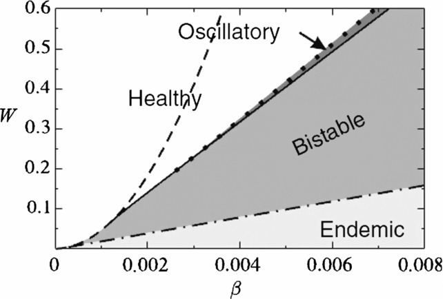
Phase diagram of a coupled disease-behavior dynamical model with an underlying network of contacts. Parameters are the rewiring rate, W, and the infection probability, β. White and light gray regions have a single attractor each, representing healthy and endemic states, respectively. Medium gray region marked “bistable” is where both of these states exhibit simultaneous stability. In the narrow dark gray region, by contrast, a stable healthy state coexists with a stable epidemic cycle. We refer to [109], from where this figure has been adapted, for further details.

An aspect of behavioral epidemiology that has received a lot of attention and more strongly relied on empirical evidence—e.g. the data on the global air transportation network [142]—is individual mobility [143], [144], [145], [146], [147], [148], [149]. Belik et al. [148], for instance, consider bidirectional motion between an origin and a destination in “individual mobility networks”. These networks capture the fact that most individuals, even if their mobility is high, frequently visit just a limited number of places, as exemplified by commuting from home to work and back. In the model, the authors embed individual mobility networks into larger networks of metapopulations, thus obtaining the results that greatly differ from those of reaction–diffusion (R-D) models. Interesting is that a propagating epidemic front exhibits saturating velocity with an increasing traveling rate, which is in sharp contrast to R-D systems. Merler et al. [146] perform a quantitative analysis of how (i) the spatial structure of the population and (ii) human mobility patterns would influence the spread of a pandemic influenza in Europe. The authors find that the high mobility of the EU population would cause an early importation of the disease from abroad, as well as synchronized local epidemics, further suggesting that the EU should be prepared for a rapid diffusion of an influenza pandemic. Sun et al. [145] resort in their analysis to a more traditional R-D approach in which a cross-diffusion term is introduced to represent the movement of the susceptibles in the direction of lower concentration of the infectives. The results show that the introduced cross-diffusion creates striped, the coexistence of striped and spotted, or just spotted patterns depending on the value of the cross-diffusion coefficient. These patterns are missing when cross-diffusion is zero, indicating that a rudimentary response of the susceptibles to the threat of infection considerably affects the disease dynamics. In addition to individual mobility, some of the most recent works focus on the heterogeneities of contact rates, for which the data from social networks (e.g. Twitter) can arguably be used as a proxy [150], [151], [152], [153]. In the context of future progress, Tizzoni et al. [153] state that an exhaustive framework for simultaneously dealing with the heterogeneities in mobility flows and contact rates is missing. Perhaps an earlier work of Eubank et al. [154] can serve as a basis for new developments in this direction.

Aside from the disease spread itself, human behavior also affects disease prevention—mainly vaccination and several non-pharmaceutical measures [155], [156], [157], [158], [159], [160], [161], [162]. Vaccination is a primary public health measure with the potential to prevent the transmission of infectious diseases, and hence reduce morbidity and mortality from infections [163], [164], [165], [166]. In most instances, vaccination is dependent on voluntary adoption rather than being enforced on the population at risk [165], [167], [168], [169], [170], [171], [172], [173], [174]. Incorporating voluntary adoption into the models of disease dynamics completes a feedback loop as illustrated in Fig. 16 . Because one feedback in this loop is positive and the other is negative, the overall dynamics may exhibit cycles, which is exactly the case when vaccination-related decision making is represented by, say, game theory or other related constructs [175], [176], [177], [178]. As vaccination coverage increases, herd immunity emerges and effectively prevents the propagation of the disease. Yet, as a consequence of the low disease prevalence, vaccination enthusiasm decreases and the high risk of infection resurfaces. The described phenomenon has been empirically observed and quantitatively verified [175]. Furthermore, if voluntary vaccination is implemented in network populations, a somewhat counterintuitive result [179], [180], [181], [182] is that heterogeneity acts to inhibit the disease outbreak. This result is due to the fact that large-degree nodes have a disproportional effect in attracting neighboring nodes to adopt vaccination [183]. Finally, vaccination can be treated in the context of an opinion formation process, which happens to impede the attainment of full herd immunity [184]. Unvaccinated clusters may emerge and dramatically increases the disease outbreak probability even if the vaccination level is generally high.

Fig. 16.

Schematic illustration of the disease-behavior dynamics forming a feedback loop. Feedback from disease to behavioral dynamics is positive (+) because an increase in disease prevalence causes an increase in perceived risk and subsequently preventive behavior. Feedback from behavioral to disease dynamics is negative (−) because an increase in preventive behavior (e.g. vaccination or other non-pharmaceutical measures) suppresses disease prevalence. The figure is reproduced from [140].

Human behavior with respect to non-pharmaceutical preventive measures—e.g. wearing face masks, frequently washing hands, distancing from the usual social circles etc.—is particularly useful in suppressing disease incidence before adequate vaccines become widely available [185]. In this context, Valdez et al. [186] consider intermittent social distancing as the primary preventive measure in a network population. Based only on local information, a susceptible agent is able to prune a link with an infectious individual with probability δ and restore it afterwards such that the underlying interaction topology remains unchanged. With the help of percolation theory, the authors find a cutoff threshold, ${\delta }_c$, directly controlling the eradication of the disease. As for the adoption of non-pharmaceutical measures, an important aspect seems to be the awareness of the current state of an infection and the associated dangers [135], [187]. The spread of awareness strengthens the behavioral response, which in turn affects the trajectory of the infection and the outbreak likelihood [188]. Finally, because non-pharmaceutical measures and vaccines go hand in hand, some recent studies consider the effectiveness of integrated frameworks that combine both of these types of prevention [157], [189]. As a concluding remark, we emphasize that coupled disease-behavior models exhibit dynamics rich with surprising phenomena, yet this richness comes at a price—models are complex and difficult to relate to the available data. Future studies should, therefore, utilize modern technologies to quantify behavioral parameters [190] and analyze the data on real-world human behavior in epidemiological contexts.

4. Pattern transitions and complexity in spatial epidemics

Pattern transitions are ubiquitous in epidemiology, yet their implications for the fate of a disease are still unclear. Here, we focus on the epidemiological role of pattern transitions in the following sense: i) if a pattern transition occurs, will the disease outbreak or die out?; and ii) if the disease outbreaks, what sort of propagation is to be expected?

4.1. Early warnings for the outbreak of infectious diseases

A stationary pattern seen in the spatial distribution of a disease implies a stable state regardless of the initial conditions [77], [78], [143]. Such a state is usually accompanied by areas in which the density of the disease is high and hence difficult to get rid off. Accordingly, transitions from one stationary pattern to another indicate that the areas of high disease density may expand or otherwise shift, meaning that the disease is about to outbreak. However, one instance in which the opposite is true is the transition from a stationary pattern to patch invasion, in which case the disease is likely to die out.

Transitions between spatio-temporal patterns can also be an early warning indicator of an imminent outbreak. Namely, spatio-temporal patterns often manifest themselves in the form of spatial chaos, which is a phenomenon predicted theoretically and observed experimentally [17], [46]. The emergence of spatial chaos, furthermore, suggests that the disease is difficult to eliminate and will persist as an endemic [17], [46].

If a mathematical model for a given disease exists, analytical methods provide the critical point(s) of the model and show when to expect sudden shift(s) towards a contrasting dynamical regime [191], [192], [193], [194], [195] (see Appendix A.3). This regime shifting is of considerable interest in other fields, including ecosystem management, population ecology, financial risk assessment, etc. [99], [196], [197], [198]. In ecosystems, for instance, a change in the skewness of control parameters proved to be a potential early warning signal for catastrophic regime shifts [198]. In Mediterranean arid ecosystems, the vegetation patch-size distribution obeys a power law, yet deviations from such a power law occur only at the onset of desertification, thus providing a potentially useful early warning indicator [99]. Despite their usefulness in many situations, non-linear methods may sometimes be an unnecessarily complicated tool, which is why a deep understanding of such methods is needed before they can be put to good use [197].

4.2. Coherence resonance

Coherence resonance is a phenomenon similar to stochastic resonance, yet requires no outside forcing for some intermediate level of the noise amplitude to maximize the “regularity” of a dynamical system at hand [199]. We use system (13a), (13b), (13c) to exemplify this phenomenon. Specifically, we add Gaussian noise to all of the system's parameters such that after addition $P=p+\xi$, where $p\in \{\beta ,{\tau }_I,{\tau }_R\}$. Random variable ξ is normally distributed dynamical noise with zero mean, standard deviation σ, and correlation function

$$〈{\xi }_i(h){\xi }_j(l)〉={\sigma }^2{\delta }_{ij}{\delta }_{hl},$$ (16)

where subscripts i and j mark two locations on a lattice, and h and l denote two time moments. This functional form guarantees that noise is neither correlated in space nor in time. The effect of an increasing σ is shown in Fig. 17 . Strikingly, in the no-noise model (i.e. $\sigma =0$), the system is in a disease-free state, whereas with noise, the disease is allowed to persist.

Fig. 17.

Noise as a cause of coherence resonance. (a) Density of infectious individuals is shown as a function of the standard deviation of noise σ. In the no-noise model, used parameter values yield a disease-free state, yet when noise is taken into account coherence resonance occurs. (b)–(d) Illustration of spatial patterns formed by the susceptibles (white), the infectives (red), and the recoverers (black) for β = 0.3. From (b) to (d), the value of σ is 0.15, 0.3, and 0.5, respectively. Other parameters are τ_I = 0.4 and τ_R = 1. The figure is reproduced from [89]. (For interpretation of the references to color in this figure legend, the reader is referred to the web version of this article.)

Although a pattern transition from the disease-free state to an endemic state is induced by the noise term, the fraction of infectious individuals is not a monotonic function of σ. This function is, in fact, concave, implying that an intermediate level of additive noise maximizes the infectious fraction (Fig. 17a). If noise is increased beyond this intermediate level, infectious individuals diminish in number and eventually disappear altogether. A visual confirmation of the described phenomenon using the accompanying spatial patterns is shown in Fig. 17b-d. Noise, therefore, has a dual role, i.e. to induce both the appearance and the disappearance of the disease, thus revealing that we are truly dealing with a manifestation of coherence resonance.

4.3. Cyclic evolution

Using SIRS system (13a), (13b), (13c), Boerlijst and Ballegooijen [200] devise a model in which pathogen strains with different infectious periods co-evolve and compete for susceptible hosts. Namely, this co-evolution and competition is achieved by assuming a mutating pathogen such that a certain fraction of new infections (determined by the mutation rate) leads with equal probability to an increase or a decrease in the infectious period. The authors investigate the potential impact of a changing mutation rate on spatial pattern transitions and show that the infectious period indefinitely keeps evolving up and down in a cyclic fashion. These cycles in the selection are caused by a change in the spatial patterns from epidemic waves to irregular local outbreaks (Fig. 18 ).

Fig. 18.

Rock-scissor-paper-type cyclic evolution of three pathogen genotypes differing in infectious period. Green, yellow, and orange color indicate genotypes with the shortest, medium, and the longest infectious period, respectively. Black and blue colors indicate susceptible and recovered individuals, respectively. (a) After 50 time steps, the green genotype is winning against the yellow one. (b) Also after 50 time steps, the yellow genotype is winning against the orange one. (c) A large difference between the two genotypes leads to a qualitatively different outcome as after 250 time steps, the orange genotype is winning against the green one. (d) The spatial pattern of the infectious period after 400 time steps. The regions of irregular outbreaks (reddish hues) have partly invaded the epidemic wave regions causing the genotype with longer infectious period to dominate, whereas in other regions (greenish hues) the genotype with shorter infectious period is still prevailing. We refer to [200], from where this figure has been adapted, for further details. (For interpretation of the references to color in this figure legend, the reader is referred to the web version of this article.)

The mechanism underlying the described phenomenon of cyclic evolution is twofold. On the one hand, if the infectious period is relatively short, epidemic waves cause local extinctions of the disease by wiping out the host (susceptible) population. Among co-occurring genotypes at such a location, after a local extinction event, the genotype that is faster in causing the disease outbreak re-invades first and increases its domain of dominance. On the other hand, if the difference in the infectious period between co-occurring genotypes is too big, epidemic waves caused by the fast genotype are broken off by the slow genotype. As a consequence, the host (susceptible) population is prevented from going extinct and outbreaks become irregular. Selection then favors the genotype with a longer infectious period because this genotype is capable of causing more secondary infections.

There is evidence that cyclic evolution is a general phenomenon in spatial epidemiology. For example, cyclic evolution is found in SEIRS models [45] and epidemiological systems with noise [201]. These examples outline the elements of a more detailed mathematical framework with which the ubiquity of cyclic evolution in spatial epidemiology could be confirmed.

5. Conclusion and future prospects

This review systematically surveys three aspects of pattern transitions in spatial epidemiology. First are discussed the examples of transitions between the two common types of patterns, spatial and spatio-temporal. Then the focus is put on the underlying causes of such pattern transitions, including spatial heterogeneity, seasonality and noise, and human behavior. Finally, potential interpretations are offered to put pattern transitions into the context of early warning indicators and other complexities arising in spatially explicit settings. We saw that stationary patterns correspond to the stable solutions of model equations, whereas spatio-temporal patterns represent either (i) quasi-periodic or oscillatory waves, (ii) temporal or spatio-temporal chaos, or even (iii) turbulence.

Although our focus is on epidemiology, the reviewed results may be useful in other realms, such as medical science, ecology, and economics. Taking cardiac disease as an example, the two frequently observed patterns in the heart are target and spiral waves [202], [203], [204]. If a target wave pattern changes to the spiral wave one, the heart rate of patients suffering from cardiac disease notably increases, causing potentially dangerous fibrillation. The evidence of transitions between spatio-temporal patterns in heart disease patients, therefore, make certain aspects of the reviewed results transferable from an epidemiological domain to the study of cardiac disease.

One weakness identifiable in many (but not all) of the reviewed results is that they are based on the following assumptions: (i) space is homogeneous and (ii) the motion of individuals is random and isotropic. However, the real-world environments are heterogeneous and heterogeneity affects human motion. In the context of the transmission dynamics, spatial heterogeneity is important because it typically decreases the invasion threshold and induces the outbreak of a disease [205]. Accordingly, with the increasing availability of individual-level high-resolution data, incorporating inhomogeneities into the models of disease spreading is becoming a priority [206]. Generic reaction–diffusion models are mainly concerned with the horizontal and possibly the vertical transmission of diseases [207], corresponding mostly to the expansion and contagious diffusion in the classification of Cromley and McLafferty [208]. Future models, however, need to consider mixed diffusion modes; in addition to the contagious diffusion thorough direct contacts, HIV is an example of a disease that spreads by means of the hierarchical diffusion from large urban areas to smaller communities, as well as the network diffusion driven by social and transportation networks. These alternative diffusion modes are especially needed if the models are to assimilate newly available data such as the data from geographic information systems, nowadays better known as simply GIS.

The additional diffusion modes mentioned above lead to geographically distant (i.e. non-local) dispersal of diseases. The hierarchical diffusion, for example, means that a disease like HIV may spread between large cities sooner than from a large city of origin to its more rural surroundings [208]. The same holds for the network diffusion as well. Such distant dispersals are difficult, if not impossible, to capture using reaction–diffusion and cellular automata models on which we focused herein. For this reason, we did mention some of the most important results in epidemiology obtained from network models, yet there is much potential for further development in this direction [209], [210], [211], [212], [213], [214], [215], [216]. Moreover, dispersal kernel functions [217], [218] offer another way to quantify the distance traveled by either susceptible or infectious individuals. To capture long-distance dispersal in particular, using leptokurtic (i.e. fat-tailed) distributions may be necessary. However, estimating the parameters of these distributions from the data is a challenging task warranting some caution [219], [220].

Throughout the paper, we described the most well-known stationary and spatio-temporal patterns and the transitions thereof that appear in epidemiology. As of lately, however, some novel types of transitions can be found in the literature. In the presence of the Allee effect, for example, transitions from stationary patterns to patch invasion are being uncovered [48]. Furthermore, transitions from stationary patterns to wave patterns may be induced by time delays or equal diffusion coefficients for susceptible, infectious, and recovered compartments [46], [221], [222]. Given that pattern transitions may serve as an early warning signal for disease outbreaks, it is of utmost importance to check the universality of these transitions for a wide variety of infections, e.g. seasonal influenza and the slew of emerging infectious diseases. Checking such universality is a formidable task, one that must be based on ample empirical evidence and in-depth interdisciplinary collaborations.

Speaking of the empirical evidence and interdisciplinary research, data science and in particular the “big data” paradigm may offer new ways to track, understand, and control infectious diseases [223], [224], [225]. One example in this context would be applying GIS to store, analyze, and process the spatial information on the propagation of an infectious disease [226], [227]. In this manner, it may be relatively easy to capture both temporal and spatial changes in the disease transmission dynamics. The ultimate goal would be to devise early warning systems based on the dynamical models capable of assimilating GIS (and other) data such that predicting the future course of the disease and recommending the effective control measures finally becomes a reality.

Communicated by V.M. Kenkre

Appendix A.

A.1. Derivation of the Laplacian operator, ${\mathrm{\nabla }}^2$

Random movements of individuals in space can be described using the Laplacian operator. Limiting ourselves to one-dimensional space, random walk assumes that, at each moment △t, an individual moves one step △x to their left or right side along a line. If initially ($t_0$) the individual is located at $x_0$, then after one time step (i.e. $t_0+△t$), the individual will move to either $x_0-△x$ or $x_0+△x$ with equal probability. Define $P(t,x)$ as the number (or the density) of individuals at time t and location x. We have

$$P(t+△t,x)=\frac{1}{2}P(t,x-△x)+\frac{1}{2}P(t,x+△x).$$ (17)

Taylor expansion gives

$$P(t+△t,x)=P(t,x)+\frac{\partial P}{\partial t}(t,x)△t+\frac{1}{2}\frac{{\partial }^{2}P}{\partial t^2}(t,x){(△t)}^2+...,$$ (18a)

$$P(t,x-△x)=P(t,x)+\frac{\partial P}{\partial x}(t,x)(-△x)+\frac{1}{2}\frac{{\partial }^{2}P}{\partial x^2}(t,x){(-△x)}^2+...,$$ (18b)

$$P(t,x+△x)=P(t,x)+\frac{\partial P}{\partial x}(t,x)(△x)+\frac{1}{2}\frac{{\partial }^{2}P}{\partial x^2}(t,x){(△x)}^2+...,$$ (18c)

which yields

$$\frac{\partial P}{\partial t}(t,x)△t+...=\frac{1}{2}\frac{{\partial }^{2}P}{\partial x^2}(t,x){(△x)}^2+....$$ (19)

Because △t and △x are small, the higher order terms are very close to zero. Consequently,

$$\frac{\partial P}{\partial t}(t,x)△t=\frac{1}{2}\frac{{\partial }^{2}P}{\partial x^2}(t,x){(△x)}^2.$$ (20)

Under the assumptions

$$△t\to 0,△x\to 0,\frac{{(△x)}^2}{2△t}\to D,$$ (21)

we obtain

$$\frac{\partial P}{\partial t}(t,x)=D\frac{{\partial }^{2}P}{\partial x^2}(t,x).$$ (22)

The derivation in two-dimensional space is completely analogous.

A.2. Standard multiple scale analysis of Eqs. (5)

By assuming the constant total population size, system (5) becomes two dimensional and we just need to consider the first two equations. Without diffusion, the positive equilibrium of Eqs. (5) is

$$\begin{array}{cc}\hfill E^{⁎}(S^{⁎},I^{⁎})=(& \frac{A\beta -\sqrt{A^2{\beta }^2-4d^3\beta -8d^2\beta (\mu +\gamma )-4d\beta {(\mu +\gamma )}^2}}{2d\beta },\hfill \\ \hfill & \frac{2d(d+\mu +\gamma )}{A\beta -\sqrt{A^2{\beta }^2-4d^3\beta -8d^2\beta (\mu +\gamma )-4d\beta {(\mu +\gamma )}^2}}).\hfill \end{array}$$

Close to the Turing threshold ($\beta ={\beta }_T$), the eigenvalues associated with the critical modes are approximately zero. These modes are slowly varying, implying that we only need to consider perturbations κ around ${\kappa }_T$. To deduce the amplitude equation, we first write the linearized form of Eqs. (5) at the equilibrium $E^{⁎}$

$$\frac{\partial u}{dt}=a_{11}u+a_{12}v-2\beta I^{⁎}uv-\beta S^{⁎}{v}^2-\beta u{v}^2+D_1{\mathrm{\Delta }}^{2}u,$$ (23a)

$$\frac{\partial v}{dt}=a_{21}u+a_{22}v+2\beta I^{⁎}uv+\beta S^{⁎}{v}^2+\beta u{v}^2+D_2{\mathrm{\Delta }}^{2}v.$$ (23b)

Close to $\beta ={\beta }_T$, the solution of the above model can be expanded as

$$\mathit{U}={\mathit{U}}_S+\sum _{j=1}^3{\mathit{U}}_0[A_j\exp (i{\overrightarrow{\kappa }}_j\cdot \overrightarrow{r})+\overline{A_j}\exp (-i{\overrightarrow{\kappa }}_j\cdot \overrightarrow{r})],$$ (24)

where $A_j$ and the conjugate $\overline{A_j}$ are the amplitudes associated with modes ${\overrightarrow{\kappa }}_j$ and $-{\overrightarrow{\kappa }}_j$, respectively. Using the standard multiple-scale analysis, the evolution of amplitudes in time and space is given by

$${\tau }_0\frac{\partial A_1}{dt}=\xi A_1+h{A}_2{A}_3-(g_1|A_1{|}^2+g_2(|A_2{|}^2+|A_3{|}^2))A_1,$$ (25a)

$${\tau }_0\frac{\partial A_2}{dt}=\xi A_2+h{A}_1{A}_3-(g_1|A_2{|}^2+g_2(|A_1{|}^2+|A_3{|}^2))A_2,$$ (25b)

$${\tau }_0\frac{\partial A_3}{dt}=\xi A_3+h{A}_1{A}_2-(g_1|A_3{|}^2+g_2(|A_1{|}^2+|A_2{|}^2))A_3,$$ (25c)

where $\xi =({\beta }_T-\beta )/{\beta }_T$ is a normalized distance and ${\tau }_0$ is a typical relaxation time. In what follows, we focus on the calculations of coefficients ${\tau }_0$, h, $g_1$ and $g_2$.

Setting $\mathit{X}={(u,v)}^T$, $\mathit{N}=(N_1,N_2)$, system (23a), (23b) is converted to

$$\frac{\partial \mathit{X}}{\partial t}=\mathit{L}\mathit{X}+\mathit{N},$$ (26)

where

$$\begin{array}{c}\mathit{L}=\left(\begin{array}{cc}\hfill a_{11}+D_1{\mathrm{\nabla }}^2\hfill & \hfill a_{12}\hfill \\ \hfill a_{21}\hfill & \hfill a_{22}+D_2{\mathrm{\nabla }}^2\hfill \end{array}\right),\hfill \\ \mathit{N}=\left(\begin{array}{c}\hfill -2\beta I^{⁎}uv-\beta S^{⁎}{v}^2-\beta u{v}^2\hfill \\ \hfill 2\beta I^{⁎}uv+\beta S^{⁎}{v}^2+\beta u{v}^2\hfill \end{array}\right).\hfill \end{array}$$

We are just interested in the dynamics when $\beta ={\beta }_T$. To that end, we expand β as

$${\beta }_T-\beta =\epsilon {\beta }_1+{\epsilon }^2{\beta }_2+{\epsilon }^3{\beta }_3+O({\epsilon }^4),$$ (27)

where ε is a small parameter. Further expanding X and the nonlinear term, N, into series around ε

$$\mathit{X}=\left(\begin{array}{c}\hfill u\hfill \\ \hfill v\hfill \end{array}\right)=\epsilon \left(\begin{array}{c}\hfill u_1\hfill \\ \hfill v_1\hfill \end{array}\right)+{\epsilon }^2\left(\begin{array}{c}\hfill u_2\hfill \\ \hfill v_2\hfill \end{array}\right)+{\epsilon }^3\left(\begin{array}{c}\hfill u_3\hfill \\ \hfill v_3\hfill \end{array}\right)+O({\epsilon }^4),$$ (28)

$$\mathit{N}={\epsilon }^2{\mathit{h}}^2+{\epsilon }^3{\mathit{h}}^3+O({\epsilon }^4),$$ (29)

where ${\mathit{h}}^2$ and ${\mathit{h}}^3$ correspond to the second and the third order of ε in the expansion of nonlinear term N. Linear operator L can be expanded as follows

$$\mathit{L}={\mathit{L}}_T+({\beta }_T-\beta )\mathit{M},$$ (30)

with

$${\mathit{L}}_T=\left(\begin{array}{cc}\hfill a_{11}^{⁎}+D_1{\mathrm{\nabla }}^2\hfill & \hfill a_{12}^{⁎}\hfill \\ \hfill a_{21}^{⁎}\hfill & \hfill a_{22}^{⁎}+D_2{\mathrm{\nabla }}^2\hfill \end{array}\right),\mathit{M}=\left(\begin{array}{cc}\hfill b_{11}\hfill & \hfill b_{12}\hfill \\ \hfill b_{21}\hfill & \hfill b_{22}\hfill \end{array}\right).$$

The core of the standard multiple-scale analysis is to separate the dynamical behavior of the system according to different temporal and spatial scales. We need to separate the time scales for system (26) (i.e. $T_0=t$, $T_1=\epsilon t$ and $T_2={\epsilon }^{2}t$). Each time scale $T_i$ can be considered as an independent variable so that the derivative of $T_i$ (with respect to time) turns into

$$\frac{\partial }{\partial t}=\frac{\partial }{\partial T_0}+\epsilon \frac{\partial }{\partial T_1}+{\epsilon }^2\frac{\partial }{\partial T_2}+O({\epsilon }^3).$$ (31)

Because the variation of the amplitude A is slow, the derivative with respect to time $\frac{\partial }{\partial T_0}$ almost has no effect on the amplitude A. Correspondingly, the above equation becomes

$$\frac{\partial A}{\partial t}=\epsilon \frac{\partial A}{\partial T_1}+{\epsilon }^2\frac{\partial A}{\partial T_2}+O({\epsilon }^3).$$ (32)

Substituting the equations (28), (29), (30), and (31) into system (26), we obtain three equations as follows.

The first order in ε:

$${\mathit{L}}_T\left(\begin{array}{c}\hfill u_1\hfill \\ \hfill v_1\hfill \end{array}\right)=0;$$

The second order in ε:

$${\mathit{L}}_T\left(\begin{array}{c}\hfill u_2\hfill \\ \hfill v_2\hfill \end{array}\right)=\frac{\partial }{\partial T_1}\left(\begin{array}{c}\hfill u_1\hfill \\ \hfill v_1\hfill \end{array}\right)-{\beta }_1\mathit{M}\left(\begin{array}{c}\hfill u_1\hfill \\ \hfill v_1\hfill \end{array}\right)-\left(\begin{array}{c}\hfill -2\beta I^{⁎}{u}_1{v}_1-\beta S^{⁎}{v}_1^2\hfill \\ \hfill 2\beta I^{⁎}{u}_1{v}_1+\beta S^{⁎}{v}_1^2\hfill \end{array}\right);$$

The third order in ε:

$$\begin{array}{c}\hfill {\mathit{L}}_T\left(\begin{array}{c}\hfill u_3\hfill \\ \hfill v_3\hfill \end{array}\right)=\frac{\partial }{\partial T_1}\left(\begin{array}{c}\hfill u_2\hfill \\ \hfill v_2\hfill \end{array}\right)+\frac{\partial }{\partial T_2}\left(\begin{array}{c}\hfill u_1\hfill \\ \hfill v_1\hfill \end{array}\right)-{\beta }_1\mathit{M}\left(\begin{array}{c}\hfill u_2\hfill \\ \hfill v_2\hfill \end{array}\right)-{\beta }_2\mathit{M}\left(\begin{array}{c}\hfill u_1\hfill \\ \hfill v_1\hfill \end{array}\right)-P,\end{array}$$ (33)

where

$$P=\left(\begin{array}{c}\hfill -2\beta I^{⁎}(u_1{v}_2+v_1{u}_2)-2\beta S^{⁎}{v}_1{v}_2-\beta u_1{v}_1^2\hfill \\ \hfill 2\beta I^{⁎}(u_1{v}_2+v_1{u}_2)+2\beta S^{⁎}{v}_1{v}_2+\beta u_1{v}_1^2\hfill \end{array}\right).$$

For the first order in ε, because ${\mathit{L}}_T$ is the linear operator of the reduced system close to the initial point, vector ${(u_1,v_1)}^T$ is a linear combination of the eigenvectors corresponding to the eigenvalue 0. We therefore obtain

$$\left(\begin{array}{c}\hfill u_1\hfill \\ \hfill v_1\hfill \end{array}\right)=\left(\begin{array}{c}\hfill \frac{a_{11}^{⁎}{D}_2-a_{22}^{⁎}{D}_1}{2a_{21}^{⁎}{D}_1}\hfill \\ \hfill 1\hfill \end{array}\right)(W_1\exp (i{\overrightarrow{\kappa }}_1\overrightarrow{r})+W_2\exp (i{\overrightarrow{\kappa }}_2\overrightarrow{r})+W_3\exp (i{\overrightarrow{\kappa }}_3\overrightarrow{r}))+c.c.,$$ (34)

where $|{\overrightarrow{\kappa }}_j|={\kappa }_T^{⁎}$ and $W_j$ is the unknown modulus of $\exp (i{\overrightarrow{\kappa }}_j\overrightarrow{r})$ under the first order perturbation. The form of $W_j$ is determined by higher order perturbations.

For the second-order differential equation in ε, we assume

$$\begin{array}{cccc}\hfill {\mathit{L}}_T\left(\begin{array}{c}\hfill u_2\hfill \\ \hfill v_2\hfill \end{array}\right)=& \frac{\partial }{\partial T_1}\left(\begin{array}{c}\hfill u_1\hfill \\ \hfill v_1\hfill \end{array}\right)-{\beta }_{1}M\left(\begin{array}{c}\hfill u_1\hfill \\ \hfill v_1\hfill \end{array}\right)\hfill & \hfill -\left(\begin{array}{c}\hfill -2\beta I^{⁎}{u}_1{v}_1-\beta S^{⁎}{v}_1^2\hfill \\ \hfill 2\beta I^{⁎}{u}_1{v}_1+\beta S^{⁎}{v}_1^2\hfill \end{array}\right)=& \left(\begin{array}{c}\hfill F_u\hfill \\ \hfill F_v\hfill \end{array}\right).\hfill \end{array}$$ (35)

To ensure a nontrivial solution, the vector function on the right hand of equation (35) must be orthogonal with the zero eigenvectors of operator ${\mathit{L}}_c^{+}$. ${\mathit{L}}_c^{+}$ is the adjoint operator of ${\mathit{L}}_c$. In this system, the zero eigenvectors of operator ${\mathit{L}}_c^{+}$ are

$$\left(\begin{array}{c}\hfill 1\hfill \\ \hfill -\frac{a_{11}^{⁎}{D}_2-a_{22}^{⁎}{D}_1}{2a_{21}^{⁎}{D}_2}\hfill \end{array}\right)\exp (-i{\overrightarrow{\kappa }}_j\overrightarrow{r})+c.c.(j=1,2,3).$$ (36)

From the orthogonality condition, we get

$$(1,-\frac{a_{11}^{⁎}{D}_2-a_{22}^{⁎}{D}_1}{2a_{21}^{⁎}{D}_2})\left(\begin{array}{c}\hfill F_u^i\hfill \\ \hfill F_v^i\hfill \end{array}\right)=0,$$ (37)

where $F_u^i$ and $F_v^i$ represent the coefficients corresponding to $\exp (i{\overrightarrow{\kappa }}_j\overrightarrow{r})$ in $F_u$ and $F_v$. Taking $\exp (i{\overrightarrow{\kappa }}_1\overrightarrow{r})$ for example, we have

$$(1-\frac{D_1}{D_2})\frac{\partial W_1}{\partial T_1}={\beta }_1(l{b}_{11}+b_{12}-\frac{\partial D_1}{\partial D_2}l(b_{21}+b_{22}))W_1-(1+\frac{D_1}{D_2}l)(4l{\beta }_T{I}^{⁎}+2l{\beta }_T{S}^{⁎}){\overline{W}}_2{\overline{W}}_3.$$ (38)

Based on the Fredholm solubility condition, we further get

$$\begin{array}{cc}\hfill \frac{D_2-D_1}{D_2}l\frac{\partial W_1}{\partial T_1}+\frac{D_2-D_1}{D_2}l\frac{\partial Y_1}{\partial T_2}& ={\beta }_2(l{b}_{11}+b_{12}-\frac{D_1}{D_2}l(l{b}_{21}+b_{22}))W_1\hfill \\ \hfill & +{\beta }_1(l{b}_{11}+b_{12}-\frac{D_1}{D_2}l(l{b}_{21}+b_{22}))Y_1\hfill \\ \hfill & +(1+\frac{D_1}{D_2}l)(4{\beta }_T{I}^{⁎}+2{\beta }_T{S}^{⁎})({\overline{W}}_3{\overline{Y}}_2+{\overline{W}}_2{\overline{Y}}_3)\hfill \\ \hfill & -(G_1|W_1{|}^2+G_2(|W_2{|}^2+|W_3{|}^2))W_1.\hfill \end{array}$$ (39)

In a similar way, other two missing equations can be obtained, meaning that amplitudes $A_i$ can be expanded as

$$A_i=\epsilon W_i+{\epsilon }^2{V}_i+O({\epsilon }^3).$$ (40)

Using Eqs. (38) and (39), multiplying by ${\epsilon }^2$ and ${\epsilon }^3$, and combining with Eqs. (32) and (40), we see that the system (25a), (25b), (25c) is indeed recovered.

A.3. Mathematical analysis of critical transitions

To exemplify the analysis of critical transitions, we take a typical SIS model [228]

$$\begin{array}{cc}\hfill & \frac{dS}{dt}=B-dS-h(v)S,\hfill \\ \hfill & \frac{dI}{dt}=h(v)S-(d+\theta )I,\hfill \\ \hfill & \frac{dv}{dt}=\delta I-\mu v,\hfill \end{array}$$ (41)

where S, I, and v represent susceptible hosts, infectious hosts, and free parasites, respectively. B is the birth rate of the susceptibles, d is the natural death rate of hosts, θ is the per capita infection-related death rate, δ is the release rate of free virus from an infected host, and a sigmoidal function, $h(v)$, is the rate of infection per host such that

$$h(v)=\frac{{(v/m_0)}^k}{1+{(v/m_1)}^k},k>1.$$ (42)

Based on the quasi-steady-state assumption, $\frac{dv}{dt}=0$, system (41) simplifies to

$$\begin{array}{cc}\hfill & \frac{dS}{dt}=B-dS-\frac{\beta I^k}{1+\alpha I^k}S,\hfill \\ \hfill & \frac{dI}{dt}=\frac{\beta I^k}{1+\alpha I^k}S-(d+\theta )I,\hfill \end{array}$$ (43)

where $\alpha ={[\delta /(\mu m_1)]}^k$ and $\beta ={[\delta /(\mu m_0)]}^k$.

As shown in Fig. A.1 , system (43) may have three equilibrium states for the same value of parameter β. In this case, a small perturbation around tipping point P may trigger different dynamical regimes—the fraction of infectious individuals may converge either to a disease-free equilibrium or a stable endemic equilibrium. Approaching the bifurcation point, P, issues an early warning signal that system (43) is about to undergo an abrupt change [191].

Fig. A.1.

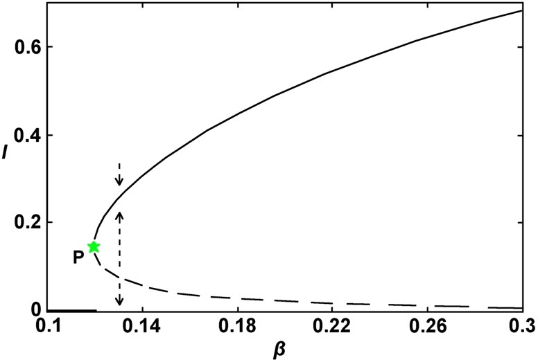
Equilibrium states of system (43) as a function of parameter β. If system (43) is very close to the bifurcation point (marked by P), then a tiny change in the parameter value may induce an abrupt shift of the system's state. Black and blue curves respectively correspond to a disease-free and an endemic equilibrium. Solid part of the blue curve indicates stable solutions, whereas dotted part indicates unstable solutions. Parameter values are B = 0.6, d = 0.05, α = 4, k = 1.42, and θ = 0.4. (For interpretation of the references to color in this figure, the reader is referred to the web version of this article.)

Assuming that system (43) has equilibrium state $E^{⁎}=(S^{⁎},I^{⁎})$, we make substitutes $S=S^{⁎}+s$ and $I=I^{⁎}+i$. Then the linearized version of this system becomes

$$\begin{array}{cc}\hfill & \frac{ds}{dt}=a_{11}s+a_{12}i,\hfill \\ \hfill & \frac{di}{dt}=a_{21}s+a_{22}i,\hfill \end{array}$$ (44)

where the Jacobian corresponding to equilibrium point $E^{⁎}$ is

$$J=\left(\begin{array}{cc}\hfill a_{11}\hfill & \hfill a_{12}\hfill \\ \hfill a_{21}\hfill & \hfill a_{22}\hfill \end{array}\right).$$

If conditions $a_{11}+a_{22}<0$ and $a_{11}{a}_{22}-a_{12}{a}_{21}>0$ are satisfied, then equilibrium state $E^{⁎}$ is stable.

A.4. Abbreviations

In Table 1 , we provide a summary of abbreviations used in the text.

Table 1.

Abbreviations used in the text.

Full name	Abbreviation
Susceptible–Infectious	SI
Susceptible–Infectious–Susceptible	SIS
Susceptible–Infectious–Removed	SIR
Susceptible–Infectious–Removed–Susceptible	SIRS
Susceptible–Exposed–Infectious–Removed–Susceptible	SEIRS
Cellular Automata	CA
Reaction–Diffusion	R-D
Ordinary Differential Equations	ODEs
Partial Differential Equations	PDEs
Human Immunodeficiency Virus	HIV
Hepatitis B Virus	HBV
Severe Acute Respiratory Syndrome	SARS
Middle East Respiratory Syndrome coronavirus	MERS-CoV
Geographic Information System	GIS

References

- 1.Neumann G., Noda T., Kawaoka Y. Emergence and pandemic potential of swine-origin H1N1 influenza virus. Nature. 2009;459:931–939. doi: 10.1038/nature08157. [DOI] [PMC free article] [PubMed] [Google Scholar]
- 2.Liu D., Shi W.F., Shi Y., Wang D.Y. Origin and diversity of novel avian influenza A H7N9 viruses causing human infection: phylogenetic, structural, and coalescent analyses. Lancet. 2013;381:1926–1932. doi: 10.1016/S0140-6736(13)60938-1. [DOI] [PubMed] [Google Scholar]
- 3.Kucharski A., Edmunds W. Case fatality rate for Ebola virus disease in West Africa. Lancet. 2014;384:1260. doi: 10.1016/S0140-6736(14)61706-2. [DOI] [PubMed] [Google Scholar]
- 4.Xia Z.-Q., Wang S.-F., Li S.-L., Huang L.-Y., Zhang W.-Y., Sun G.-Q. Modeling the transmission dynamics of Ebola virus disease in Liberia. Sci Rep. 2015;5:13857. doi: 10.1038/srep13857. [DOI] [PMC free article] [PubMed] [Google Scholar]
- 5.Corti D., Zhao J., Pedotti M., Simonelli L., Agnihothram S., Fett C. Prophylactic and postexposure efficacy of a potent human monoclonal antibody against MERS coronavirus. Proc Natl Acad Sci USA. 2015;112:10473–10478. doi: 10.1073/pnas.1510199112. [DOI] [PMC free article] [PubMed] [Google Scholar]
- 6.Bernoulli D. Memories de Mathématiques et de physique. Académie Royale des Sciences; Paris: 1760. Essai d'une nouvelle analyse de la mortalité causee par la petite verole et des avantages de l'inoculation pour al prevenir; pp. 1–45. [Google Scholar]
- 7.Hamer W. Epidemic disease in England: the evidence of variability and the persistence of type. Lancet. 1906;167:733–739. [Google Scholar]
- 8.Ross R. Murray; London: 1911. The prevention of malaria. [Google Scholar]
- 9.Kermack W.O., McKendrick W.O. A contribution to the mathematical theory of epidemics. Proc R Soc Lond A. 1927;115:700–721. [Google Scholar]
- 10.Abbey H. An examination of the Reed–Frost theory of epidemics. Hum Biol. 1952;24(3):201–233. [PubMed] [Google Scholar]
- 11.Anderson R.M., May R.M. Oxford University Press; Oxford: 1992. Infectious diseases of humans. [Google Scholar]
- 12.Diekmann O., Heesterbeek J. Wiley; New York: 2000. Mathematical epidemiology of infectious diseases: model building, analysis and interpretation. [Google Scholar]
- 13.Keeling M.J., Rohani P. Princeton University Press; Princeton: 2007. Modeling infectious diseases in humans and animals. [Google Scholar]
- 14.Li M.-T., Sun G.-Q., Wu Y.-F., Zhang J., Jin Z. Transmission dynamics of a multi-group brucellosis model with mixed cross infection in public farm. Appl Math Comput. 2014;237:582–594. [Google Scholar]
- 15.Sun G.-Q., Zhang Z.-K. Global stability for a sheep brucellosis model with immigration. Appl Math Comput. 2014;246:336–345. [Google Scholar]
- 16.Keeling M., Grenfell B. Disease extinction and community size: modeling the persistence of measles. Science. 1997;275:65–67. doi: 10.1126/science.275.5296.65. [DOI] [PubMed] [Google Scholar]
- 17.Gupta S., Ferguson N., Anderson R. Chaos, persistence, and evolution of strain structure in antigenically diverse infectious agents. Science. 1998;280:912–915. doi: 10.1126/science.280.5365.912. [DOI] [PubMed] [Google Scholar]
- 18.Earn D., Dushoff J., Levin S. Ecology and evolution of the flu. Trends Ecol Evol. 2002;17:334–340. [Google Scholar]
- 19.Martin R., Smith H. Abstract functional differential equations and reaction–diffusion systems. Trans Am Math Soc. 1990;321:1–44. [Google Scholar]
- 20.Carr J., Chmaj A. Uniqueness of travelling waves for nonlocal monostable equations. Proc Am Math Soc. 2004;132:2433–2439. [Google Scholar]
- 21.Faria T., Huang W., Wu J. Travelling waves for delayed reaction–diffusion equations with global response. Proc R Soc Lond Ser A. 2006;462:229–261. [Google Scholar]
- 22.Wang Z.-C., Li W.-T., Ruan S. Existence and stability of traveling wave fronts in reaction advection diffusion equations with nonlocal delay. J Differ Equ. 2007;238:153–200. [Google Scholar]
- 23.Ouyang Q., Flesselles J.-M. Transition from spirals to defect turbulence driven by a convective instability. Nature. 1996;379:143–146. [Google Scholar]
- 24.Fuentes M.A., Kuperman M.N., Kenkre V.M. Nonlocal interaction effects on pattern formation in population dynamics. Phys Rev Lett. 2003;91 doi: 10.1103/PhysRevLett.91.158104. [DOI] [PubMed] [Google Scholar]
- 25.Fuentes M.A., Kuperman M.N., Kenkre V.M. Analytical considerations in the study of spatial patterns arising from nonlocal interaction effects. J Phys Chem B. 2004;108:10505–10508. [Google Scholar]
- 26.Cross M.C., Hohenberg P.C. Pattern formation outside of equilibrium. Rev Mod Phys. 1993;65:851–1112. [Google Scholar]
- 27.Clerc M.G., Escaff D., Kenkre V.M. Patterns and localized structures in population dynamics. Phys Rev E. 2005;72 doi: 10.1103/PhysRevE.72.056217. [DOI] [PubMed] [Google Scholar]
- 28.Kumar N., Parmenter R.R., Kenkre V.M. Extinction of refugia of hantavirus infection in a spatially heterogeneous environment. Phys Rev E. 2010;82 doi: 10.1103/PhysRevE.82.011920. [DOI] [PubMed] [Google Scholar]
- 29.Rhodes C., Anderson R. Dynamics in a lattice epidemic model. Phys Lett A. 1996;201:183–188. [Google Scholar]
- 30.Willox R., Grammaticos B., Carstea A., Ramani A. Epidemic dynamics: discrete-time and cellular automaton models. Physica A. 2003;328:13–22. [Google Scholar]
- 31.Fuentes M., Kuperman M. Cellular automata and epidemiological models with spatial dependence. Physica A. 1999;267:471–486. [Google Scholar]
- 32.Nichol S., Spiropoulou C., Morzunov S., Rollin P., Ksiazek T., Feldmann H. Genetic identification of a hantavirus associated with an outbreak of acute respiratory illness. Science. 1993;262:914–917. doi: 10.1126/science.8235615. [DOI] [PubMed] [Google Scholar]
- 33.Parmenter C.A., Yates T.L., Parmenter R.R., Dunnum J.L. Statistical sensitivity for detection of spatial and temporal patterns in rodent population densities. Emerg Infect Dis. 1999;5:118–125. doi: 10.3201/eid0501.990114. [DOI] [PMC free article] [PubMed] [Google Scholar]
- 34.Abramson G., Kenkre V.M. Spatiotemporal patterns in the hantavirus infection. Phys Rev E. 2002;66 doi: 10.1103/PhysRevE.66.011912. [DOI] [PubMed] [Google Scholar]
- 35.Kenkre V.M. Statistical mechanical considerations in the theory of the spread of the hantavirus. Physica A. 2005;356:121–126. [Google Scholar]
- 36.Kenkre V., Giuggioli L., Abramson G., Camelo-Neto G. Theory of hantavirus infection spread incorporating localized adult and itinerant juvenile mice. Eur Phys J B. 2007;55:461–470. [Google Scholar]
- 37.Fisher R.A. The wave of advance of advantageous genes. Ann Eug. 1937;7:355–369. [Google Scholar]
- 38.Gubler D.J. Epidemic dengue/dengue hemorrhagic fever as a public health, social and economic problem in the 21st century. Trends Microbiol. 2002;10:100–103. doi: 10.1016/s0966-842x(01)02288-0. [DOI] [PubMed] [Google Scholar]
- 39.Grassly N.C., Fraser C., Wenger J., Deshpande J.M., Sutter R.W., Heymann D.L. New strategies for the elimination of polio from India. Science. 2006;314:1150–1153. doi: 10.1126/science.1130388. [DOI] [PubMed] [Google Scholar]
- 40.Williams B.G., Lloyd-Smith J.O., Gouws E., Hankins C., Getz W.M., Hargrove J. The potential impact of male circumcision on HIV in sub-Saharan Africa. PLoS Med. 2006;3 doi: 10.1371/journal.pmed.0030262. [DOI] [PMC free article] [PubMed] [Google Scholar]
- 41.Sun G.-Q., Jin Z., Liu Q.-X., Li L. Pattern formation in a spatial S-I model with non-linear incidence rates. J Stat Mech. 2007;11 [Google Scholar]
- 42.Sun G.-Q. Pattern formation of an epidemic model with diffusion. Nonlinear Dyn. 2012;69:1097–1104. doi: 10.1007/s11071-012-0330-5. [DOI] [PMC free article] [PubMed] [Google Scholar]
- 43.van Ballegooijen W.M., Boerlijst M.C. Emergent trade-offs and selection for outbreak frequency in spatial epidemics. Proc Natl Acad Sci USA. 2004;101:18246–18250. doi: 10.1073/pnas.0405682101. [DOI] [PMC free article] [PubMed] [Google Scholar]
- 44.Liu Q.-X., Jin Z., Liu M.-X. Spatial organization and evolution period of the epidemic model using cellular automata. Phys Rev E. 2006;74 doi: 10.1103/PhysRevE.74.031110. [DOI] [PubMed] [Google Scholar]
- 45.Liu Q.-X., Wang R.-H., Jin Z. Persistence, extinction and spatio-temporal synchronization of SIRS spatial models. J Stat Mech. 2009;07 [Google Scholar]
- 46.Sun G.-Q., Jin Z., Liu Q.-X., Li L. Chaos induced by breakup of waves in a spatial epidemic model with nonlinear incidence rate. J Stat Mech. 2008;08 [Google Scholar]
- 47.Sun G.-Q., Liu Q.-X., Jin Z., Chakraborty A., Li B.-L. Influence of infection rate and migration on extinction of disease in spatial epidemics. J Theor Biol. 2010;264:95–103. doi: 10.1016/j.jtbi.2010.01.006. [DOI] [PubMed] [Google Scholar]
- 48.Li L. Patch invasion in a spatial epidemic model. Appl Math Comput. 2015;258:342–349. [Google Scholar]
- 49.Schimit P., Monteiro L. A vaccination game based on public health actions and personal decisions. Ecol Model. 2011;222:1651–1655. [Google Scholar]
- 50.Barbera E., Consolo G., Valenti G. Spread of infectious diseases in a hyperbolic reaction–diffusion susceptible–infected–removed model. Phys Rev E. 2013;88 doi: 10.1103/PhysRevE.88.052719. [DOI] [PubMed] [Google Scholar]
- 51.Crawford B.A., Kribs-Zaleta C.M., Ambartsoumian G. Invasion speed in cellular automaton models for T. cruzi vector migration. Bull Math Biol. 2013;75:1051–1081. doi: 10.1007/s11538-013-9840-7. [DOI] [PubMed] [Google Scholar]
- 52.Su M., Hui C., Lin Z. Effects of the transmissibility and virulence of pathogens on intraguild predation in fragmented landscapes. Biosystems. 2015;129:44–49. doi: 10.1016/j.biosystems.2015.02.002. [DOI] [PubMed] [Google Scholar]
- 53.Ostfeld R., Glass G., Keesing F. Spatial epidemiology: an emerging (or re-emerging) discipline. Trends Ecol Evol. 2005;20:328–336. doi: 10.1016/j.tree.2005.03.009. [DOI] [PubMed] [Google Scholar]
- 54.Cohen M.L. Changing patterns of infectious disease. Nature. 2000;406:762–767. doi: 10.1038/35021206. [DOI] [PubMed] [Google Scholar]
- 55.Lloyd-Smith J.O., Schreiber S.J., Kopp P.E., Getz W.M. Superspreading and the effect of individual variation on disease emergence. Nature. 2005;438:355–359. doi: 10.1038/nature04153. [DOI] [PMC free article] [PubMed] [Google Scholar]
- 56.Jones K.E., Patel N.G., Levy M.A., Storeygard A., Balk D., Gittleman J.L. Global trends in emerging infectious diseases. Nature. 2008;451:990–994. doi: 10.1038/nature06536. [DOI] [PMC free article] [PubMed] [Google Scholar]
- 57.Grenfell B., Bjornstad O., Kappey J. Travelling waves and spatial hierarchies in measles epidemics. Nature. 2001;414:716–723. doi: 10.1038/414716a. [DOI] [PubMed] [Google Scholar]
- 58.Kenkre V., Kuperman M. Applicability of the Fisher equation to bacterial population dynamics. Phys Rev E. 2003;67 doi: 10.1103/PhysRevE.67.051921. [DOI] [PubMed] [Google Scholar]
- 59.Ballard M., Kenkre V., Kuperman M. Periodically varying externally imposed environmental effects on population dynamics. Phys Rev E. 2004;70 doi: 10.1103/PhysRevE.70.031912. [DOI] [PubMed] [Google Scholar]
- 60.Kenkre V., Niraj K. Nonlinearity in bacterial population dynamics: proposal for experiments for the observation of abrupt transitions in patches. Proc Natl Acad Sci. 2008;105:18752–18757. doi: 10.1073/pnas.0805215105. [DOI] [PMC free article] [PubMed] [Google Scholar]
- 61.Clerc M., Escaff D., Kenkre V. Analytical studies of fronts, colonies, and patterns: combination of the Allee effect and nonlocal competition interactions. Phys Rev E. 2010;82 doi: 10.1103/PhysRevE.82.036210. [DOI] [PubMed] [Google Scholar]
- 62.Kumar N., Kenkre V. Effects of gradual spatial variation in resources on population extinction: analytic calculations for abrupt transitions. Physica A. 2011;390:257–262. [Google Scholar]
- 63.Sun G.-Q., Zhang J., Song L.-P., Jin Z., Li B.-L. Pattern formation of a spatial predator–prey system. Appl Math Comput. 2012;218:11151–11162. [Google Scholar]
- 64.Riley S., Ferguson N. Smallpox transmission and control: spatial dynamics in Great Britain. Proc Natl Acad Sci USA. 2006;103:12637–12642. doi: 10.1073/pnas.0510873103. [DOI] [PMC free article] [PubMed] [Google Scholar]
- 65.Murray J. Springer; Berlin: 1993. Mathematical biology. [Google Scholar]
- 66.Liu W., Hethcote H., Levin S. Influence of nonlinear incidence rates upon the behaviour of SIRS epidemiological models. J Math Biol. 1986;23:187–204. doi: 10.1007/BF00276956. [DOI] [PubMed] [Google Scholar]
- 67.Liu W., Levin S., Iwasa Y. Dynamical behavior of epidemiological model with nonlinear incidence rate. J Math Biol. 1987;25:359–380. doi: 10.1007/BF00277162. [DOI] [PubMed] [Google Scholar]
- 68.Ferguson N., Keeling M., Edmunds W., Gani R., Grenfell B., Anderson R. Planning for smallpox outbreaks. Nature. 2003;425:681–685. doi: 10.1038/nature02007. [DOI] [PMC free article] [PubMed] [Google Scholar]
- 69.House T., Hall I., Danon L., Keeling M. Contingency planning for a deliberate release of smallpox in Great Britain–the role of geographical scale and contact structure. BMC Infect Dis. 2010;10:25. doi: 10.1186/1471-2334-10-25. [DOI] [PMC free article] [PubMed] [Google Scholar]
- 70.Tecle T., Bottiger B., Orvell C., Johansson B. Characterization of two decades of temporal co-circulation of four mumps virus genotypes in Denmark: identification of a new genotype. J Gen Virol. 2001;82:2675–2680. doi: 10.1099/0022-1317-82-11-2675. [DOI] [PubMed] [Google Scholar]
- 71.Amexis G., Rubin S., Chizhikov V., Pelloquin F., Carbone K., Chumakov K. Sequence diversity of Jeryl Lynn strain of mumps virus: quantitative mutant analysis for vaccine quality control. Virology. 2002;300:171–179. doi: 10.1006/viro.2002.1499. [DOI] [PubMed] [Google Scholar]
- 72.Kondo S., Miura T. Reaction–diffusion model as a framework for understanding biological pattern formation. Science. 2010;329:1616–1620. doi: 10.1126/science.1179047. [DOI] [PubMed] [Google Scholar]
- 73.Nicolis G., Prigogine I. Wiley; New York: 1977. Self-organization in nonequilibrium systems. [Google Scholar]
- 74.Gunaratne G.H., Ouyang Q., Swinney H.L. Pattern formation in the presence of symmetries. Phys Rev E. 1994;50:2802–2820. doi: 10.1103/physreve.50.2802. [DOI] [PubMed] [Google Scholar]
- 75.Pena B., Pérez-García C. Stability of Turing patterns in the Brusselator model. Phys Rev E. 2001;64 doi: 10.1103/PhysRevE.64.056213. [DOI] [PubMed] [Google Scholar]
- 76.Zhang X.-C., Sun G.-Q., Jin Z. Spatial dynamics in a predator–prey model with Beddington–DeAngelis functional response. Phys Rev E. 2012;85 doi: 10.1103/PhysRevE.85.021924. [DOI] [PubMed] [Google Scholar]
- 77.Sun G.-Q., Li L., Jin Z., Zhang Z.-K., Zhou T. Pattern dynamics in a spatial predator–prey system with Allee effect. Abstr Appl Anal. 2013;2013 [Google Scholar]
- 78.Sun G.-Q., Li L., Zhang Z.-K. Spatial dynamics of a vegetation model in an arid flat environment. Nonlinear Dyn. 2013;73:2207–2219. [Google Scholar]
- 79.Garcia-Ojalvo J., Sancho J.M. Springer; New York: 1999. Noise in spatially extended systems. [DOI] [PubMed] [Google Scholar]
- 80.Rohani P., Earn D.J., Grenfell B.T. Opposite patterns of synchrony in sympatric disease metapopulations. Science. 1999;286:968–971. doi: 10.1126/science.286.5441.968. [DOI] [PubMed] [Google Scholar]
- 81.Rohani P., Keeling M., Grenfell B. The interplay between noise and determinism in childhood diseases. Am Nat. 2002;159:469–481. doi: 10.1086/339467. [DOI] [PubMed] [Google Scholar]
- 82.Sun G.-Q., Li L., Jin Z., Li B.-L. Effect of noise on the pattern formation in an epidemic model. Numer Methods Partial Differ Equ. 2010;26:1168–1179. [Google Scholar]
- 83.Lesmes F., Hochberg D., Moran F., Perez-Mercader J. Noise-controlled self-replicating patterns. Phys Rev Lett. 2003;91 doi: 10.1103/PhysRevLett.91.238301. [DOI] [PubMed] [Google Scholar]
- 84.Li L., Jin Z. Pattern dynamics of a spatial predator–prey model with noise. Nonlinear Dyn. 2012;67:1737–1744. [Google Scholar]
- 85.Wang H., Zhang K., Ouyang Q. Resonant-pattern formation induced by additive noise in periodically forced reaction–diffusion systems. Phys Rev E. 2006;74 doi: 10.1103/PhysRevE.74.036210. [DOI] [PubMed] [Google Scholar]
- 86.Durrett R., Levin S. The importance of being discrete (and spatial) Theor Popul Biol. 1994;46:363–394. [Google Scholar]
- 87.Durrett R., Levin S. Stochastic spatial models–a user guide to ecological applications. Philos Trans R Soc Lond B. 1994;343:329–350. [Google Scholar]
- 88.Lion S., van Baalen M. Self-structuring in spatial evolutionary ecology. Ecol Lett. 2008;11:277–285. doi: 10.1111/j.1461-0248.2007.01132.x. [DOI] [PubMed] [Google Scholar]
- 89.Sun G.-Q., Jin Z., Song L.-P., Chakraborty A., Li B.-L. Phase transition in spatial epidemics using cellular automata with noise. Ecol Res. 2011;26:333–340. [Google Scholar]
- 90.Sun G.-Q., Jin Z., Li L. Emergent Turing pattern in epidemic spreading using cellular automaton. Int J Mod Phys B. 2011;25:4605–4613. [Google Scholar]
- 91.Deutsch A., Dormann S. Springer Science & Business Media; Boston: 2007. Cellular automaton modeling of biological pattern formation: characterization, applications, and analysis. [Google Scholar]
- 92.Mocroft A., Vella S., Benfield T., Chiesi A., Miller V., Gargalianos P. Changing patterns of mortality across Europe in patients infected with HIV-1. Lancet. 1998;352:1725–1730. doi: 10.1016/s0140-6736(98)03201-2. [DOI] [PubMed] [Google Scholar]
- 93.Iwami S., Nakaoka S., Takeuchi Y., Miura Y., Miura T. Immune impairment thresholds in HIV infection. Immunol Lett. 2009;123(2):149–154. doi: 10.1016/j.imlet.2009.03.007. [DOI] [PubMed] [Google Scholar]
- 94.Iwami S., Miura T., Nakaoka S., Takeuchi Y. Immune impairment in HIV infection: existence of risky and immunodeficiency thresholds. J Theor Biol. 2009;260(4):490–501. doi: 10.1016/j.jtbi.2009.06.023. [DOI] [PubMed] [Google Scholar]
- 95.Edmunds W., Medley G., Nokes C.O.D.J., Whittle H., Hall A. Epidemiological patterns of hepatitis B virus (HBV) in highly endemic areas. Epidemiol Infect. 1996;117:313–325. doi: 10.1017/s0950268800001497. [DOI] [PMC free article] [PubMed] [Google Scholar]
- 96.Klausmeier C. Regular and irregular patterns in semiarid vegetation. Science. 1999;284:1826–1828. doi: 10.1126/science.284.5421.1826. [DOI] [PubMed] [Google Scholar]
- 97.von Hardenberg J., Meron E., Shachak M., Zarmi Y. Diversity of vegetation patterns and desertification. Phys Rev Lett. 2001;87 doi: 10.1103/PhysRevLett.87.198101. [DOI] [PubMed] [Google Scholar]
- 98.Rietkerk M., Decker S., de Ruiter P., van de Koppel J. Self-organized patchiness and catastrophic shift in ecosystems. Science. 2004;305:1926–1929. doi: 10.1126/science.1101867. [DOI] [PubMed] [Google Scholar]
- 99.Kefi S., Rietkerk M., Alados C., Pueyo Y., Papanastasis V., ElAich A. Spatial vegetation patterns and imminent desertification in Mediterranean arid ecosystems. Nature. 2007;449:213–217. doi: 10.1038/nature06111. [DOI] [PubMed] [Google Scholar]
- 100.Meron E. Taylor & Francis; Boca Raton: 2015. Nonlinear physics of ecosystems. [Google Scholar]
- 101.Abramson G., Kenkre V.M., Yates T.L., Parmenter R.R. Traveling waves of infection in the hantavirus epidemics. Bull Math Biol. 2003;65:519–534. doi: 10.1016/S0092-8240(03)00013-2. [DOI] [PubMed] [Google Scholar]
- 102.Pepin K.M., Riley S., Grenfell B.T. Effects of influenza antivirals on individual and population immunity over many epidemic waves. Epidemiol Infect. 2013;141:366–376. doi: 10.1017/S0950268812000477. [DOI] [PMC free article] [PubMed] [Google Scholar]
- 103.Camacho A., Ballesteros S., Graham A.L., Carrat F., Ratmann O., Cazelles B. Explaining rapid reinfections in multiplewave influenza outbreaks: Tristan da cunha 1971 epidemic as a case study. Proc R Soc B. 2011;278:3635–3643. doi: 10.1098/rspb.2011.0300. [DOI] [PMC free article] [PubMed] [Google Scholar]
- 104.Matrajt L., Longini I.M., Jr Critical immune and vaccination thresholds for determining multiple influenza epidemic waves. Epidemics. 2012;4:22–32. doi: 10.1016/j.epidem.2011.11.003. [DOI] [PMC free article] [PubMed] [Google Scholar]
- 105.Puoti M., Girardi E. Chronic hepatitis C in Italy: the vanishing of the first and most consistent epidemic wave. Dig Liver Dis. 2013;45:369–370. doi: 10.1016/j.dld.2013.02.012. [DOI] [PubMed] [Google Scholar]
- 106.Lion S., van Baalen M., Wilson W. The evolution of parasite manipulation of host dispersal. Proc R Soc B. 2006;273:1063–1071. doi: 10.1098/rspb.2005.3412. [DOI] [PMC free article] [PubMed] [Google Scholar]
- 107.Haraguchi Y., Sasaki A. The evolution of parasite virulence and transmission rate in a spatially structured population. J Theor Biol. 2000;203:85–96. doi: 10.1006/jtbi.1999.1065. [DOI] [PubMed] [Google Scholar]
- 108.Restif O., Grenfell B.T. Integrating life history and cross-immunity into the evolutionary dynamics of pathogens. Proc R Soc B. 2006;273:409–416. doi: 10.1098/rspb.2005.3335. [DOI] [PMC free article] [PubMed] [Google Scholar]
- 109.Gross T., D'Lima C.J.D., Blasius B. Epidemic dynamics on an adaptive network. Phys Rev Lett. 2006;96 doi: 10.1103/PhysRevLett.96.208701. [DOI] [PubMed] [Google Scholar]
- 110.Gross T., Blasius B. Adaptive coevolutionary networks: a review. J R Soc Interface. 2008;5:259–271. doi: 10.1098/rsif.2007.1229. [DOI] [PMC free article] [PubMed] [Google Scholar]
- 111.Chowell G., Viboud C., Wang X., Bertozzi S.M., Miller M.A. Adaptive vaccination strategies to mitigate pandemic influenza: Mexico as a case study. PLoS ONE. 2009;4 doi: 10.1371/journal.pone.0008164. [DOI] [PMC free article] [PubMed] [Google Scholar]
- 112.Goldstein E., Wallinga J., Lipsitch M. Vaccine allocation in a declining epidemic. J R Soc Interface. 2012;9:2798–2803. doi: 10.1098/rsif.2012.0404. [DOI] [PMC free article] [PubMed] [Google Scholar]
- 113.Wang Z.-C., Wu J., Liu R. Traveling waves of the spread of avian influenza. Proc Am Math Soc. 2012;140:3931–3946. [Google Scholar]
- 114.Jewell C.P., Keeling M.J., Roberts G.O. Predicting undetected infections during the 2007 foot-and-mouth disease outbreak. J R Soc Interface. 2009;6:1145–1151. doi: 10.1098/rsif.2008.0433. [DOI] [PMC free article] [PubMed] [Google Scholar]
- 115.Su Y., Ruan S., Wei J. Periodicity and synchronization in blood-stage malaria infection. J Math Biol. 2011;63:557–574. doi: 10.1007/s00285-010-0381-5. [DOI] [PubMed] [Google Scholar]
- 116.Okubo A., Levin S.A. Springer; New York: 2001. Diffusion and ecological problems: modern perspectives. [Google Scholar]
- 117.Engbert R., Drepper F. Chance and chaos in population biology-models of recurrent epidemics and food chain dynamics. Chaos Solitons Fractals. 1994;4:1147–1169. [Google Scholar]
- 118.Lloyd A.L., May R.M. Spatial heterogeneity in epidemic models. J Theor Biol. 1996;179:1–11. doi: 10.1006/jtbi.1996.0042. [DOI] [PubMed] [Google Scholar]
- 119.Li M.Y., Shuai Z.S. Global stability of an epidemic model in a patchy environment. Can Appl Math Q. 2009;17:175–187. [Google Scholar]
- 120.Hagenaars T., Donnelly C., Ferguson N. Spatial heterogeneity and the persistence of infectious diseases. J Theor Biol. 2004;229:349–359. doi: 10.1016/j.jtbi.2004.04.002. [DOI] [PubMed] [Google Scholar]
- 121.Lloyd A.L., Jansen V.A. Spatiotemporal dynamics of epidemics: synchrony in metapopulation models. Math Biosci. 2004;188:1–16. doi: 10.1016/j.mbs.2003.09.003. [DOI] [PubMed] [Google Scholar]
- 122.Wang J-B, Wang L, Li X. Identifying spatial invasion of pandemics on metapopulation networks via anatomizing arrival history. IEEE Transaction on Cybernetics. [DOI] [PMC free article] [PubMed]
- 123.Johnson C.R., Boerlijst M.C. Selection at the level of the community: the importance of spatial structure. Trends Ecol Evol. 2002;17:83–90. [Google Scholar]
- 124.Earn D.J., Rohani P., Bolker B.M., Grenfell B.T. A simple model for complex dynamical transitions in epidemics. Science. 2000;287:667–670. doi: 10.1126/science.287.5453.667. [DOI] [PubMed] [Google Scholar]
- 125.Keeling M.J., Rohani P., Grenfell B.T. Seasonally forced disease dynamics explored as switching between attractors. Physica D. 2001;148:317–335. [Google Scholar]
- 126.Nguyen H.T., Rohani P. Noise, nonlinearity and seasonality: the epidemics of whooping cough revisited. J R Soc Interface. 2008;5:403–413. doi: 10.1098/rsif.2007.1168. [DOI] [PMC free article] [PubMed] [Google Scholar]
- 127.Dushoff J., Plotkin J.B., Levin S.A., Earn D.J. Dynamical resonance can account for seasonality of influenza epidemics. Proc Natl Acad Sci USA. 2004;101:16915–16916. doi: 10.1073/pnas.0407293101. [DOI] [PMC free article] [PubMed] [Google Scholar]
- 128.Balcan D., Hu H., Goncalves B., Bajardi P., Poletto C., Ramasco J.J. Seasonal transmission potential and activity peaks of the new influenza A (H1N1): a Monte Carlo likelihood analysis based on human mobility. BMC Med. 2009;7:45. doi: 10.1186/1741-7015-7-45. [DOI] [PMC free article] [PubMed] [Google Scholar]
- 129.Bartlett M.S. Measles periodicity and community size. J R Stat Soc A. 1957;123:48–70. [Google Scholar]
- 130.Keeling M., Grenfell B. Stochastic dynamics and a power law for measles variability. Philos Trans R Soc B. 1999;354:769–776. doi: 10.1098/rstb.1999.0429. [DOI] [PMC free article] [PubMed] [Google Scholar]
- 131.Coulson T., Rohani P., Pascual M. Skeletons, noise and population growth: the end of an old debate? Trends Ecol Evol. 2004;19:359–364. doi: 10.1016/j.tree.2004.05.008. [DOI] [PubMed] [Google Scholar]
- 132.Alonso D., McKane A.J., Pascual M. Stochastic amplification in epidemics. J R Soc Interface. 2007;4:575–582. doi: 10.1098/rsif.2006.0192. [DOI] [PMC free article] [PubMed] [Google Scholar]
- 133.Simoes M., da Gama M.T., Nunes A. Stochastic fluctuations in epidemics on networks. J R Soc Interface. 2008;5:555–566. doi: 10.1098/rsif.2007.1206. [DOI] [PMC free article] [PubMed] [Google Scholar]
- 134.Manfredi P., d'Onofrio A. Springer; New York: 2013. Modeling the interplay between human behavior and the spread of infectious diseases. [Google Scholar]
- 135.Funk S., Salathé M., Jansen V.A. Modelling the influence of human behaviour on the spread of infectious diseases: a review. J R Soc Interface. 2010;7:1247–1256. doi: 10.1098/rsif.2010.0142. [DOI] [PMC free article] [PubMed] [Google Scholar]
- 136.Ibuka Y., Chapman G.B., Meyers L.A., Li M., Galvani A.P. The dynamics of risk perceptions and precautionary behavior in response to 2009 (H1N1) pandemic influenza. BMC Infect Dis. 2010;10:296. doi: 10.1186/1471-2334-10-296. [DOI] [PMC free article] [PubMed] [Google Scholar]
- 137.Poletti P., Ajelli M., Merler S. The effect of risk perception on the 2009 H1N1 pandemic influenza dynamics. PLoS ONE. 2011;6 doi: 10.1371/journal.pone.0016460. [DOI] [PMC free article] [PubMed] [Google Scholar]
- 138.Salathé M., Khandelwal S. Assessing vaccination sentiments with online social media: implications for infectious disease dynamics and control. PLoS Comput Biol. 2011;7 doi: 10.1371/journal.pcbi.1002199. [DOI] [PMC free article] [PubMed] [Google Scholar]
- 139.SteelFisher G.K., Blendon R.J., Bekheit M.M., Lubell K. The public's response to the 2009 H1N1 influenza pandemic. N Engl J Med. 2010;362 doi: 10.1056/NEJMp1005102. [DOI] [PubMed] [Google Scholar]
- 140.Wang Z., Andrews M.A., Wu Z.-X., Wang L., Bauch C.T. Coupled disease-behavior dynamics on complex networks: a review. Phys Life Rev. 2015;15:1–29. doi: 10.1016/j.plrev.2015.07.006. [DOI] [PMC free article] [PubMed] [Google Scholar]
- 141.Van Segbroeck S., Santos F.C., Pacheco J.M. Adaptive contact networks change effective disease infectiousness and dynamics. PLoS Comput Biol. 2010;6 doi: 10.1371/journal.pcbi.1000895. [DOI] [PMC free article] [PubMed] [Google Scholar]
- 142.Colizza V., Barrat A., Barthélemy M., Vespignani A. The role of the airline transportation network in the prediction and predictability of global epidemics. Proc Natl Acad Sci USA. 2006;103:2015–2020. doi: 10.1073/pnas.0510525103. [DOI] [PMC free article] [PubMed] [Google Scholar]
- 143.Colizza V., Pastor-Satorras R., Vespignani A. Reaction–diffusion processes and metapopulation models in heterogeneous networks. Nat Phys. 2007;3:276–282. [Google Scholar]
- 144.Gonzalez M.C., Hidalgo C.A., Barabasi A.-L. Understanding individual human mobility patterns. Nature. 2008;453:779–782. doi: 10.1038/nature06958. [DOI] [PubMed] [Google Scholar]
- 145.Sun G.-Q., Jin Z., Liu Q.-X., Li L. Spatial pattern in an epidemic system with cross-diffusion of the susceptible. J Biol Syst. 2009;17:141–152. [Google Scholar]
- 146.Merler S., Ajelli M. The role of population heterogeneity and human mobility in the spread of pandemic influenza. Proc R Soc B. 2010;277:557–565. doi: 10.1098/rspb.2009.1605. [DOI] [PMC free article] [PubMed] [Google Scholar]
- 147.Meloni S., Perra N., Arenas A., Gómez S., Moreno Y., Vespignani A. Modeling human mobility responses to the large-scale spreading of infectious diseases. Sci Rep. 2011;1:62. doi: 10.1038/srep00062. [DOI] [PMC free article] [PubMed] [Google Scholar]
- 148.Belik V., Geisel T., Brockmann D. Natural human mobility patterns and spatial spread of infectious diseases. Phys Rev X. 2011;1 [Google Scholar]
- 149.Poletto C., Tizzoni M., Colizza V. Heterogeneous length of stay of hosts' movements and spatial epidemic spread. Sci Rep. 2012;2:476. doi: 10.1038/srep00476. [DOI] [PMC free article] [PubMed] [Google Scholar]
- 150.Newman M. Spread of epidemic disease on networks. Phys Rev E. 2002;66 doi: 10.1103/PhysRevE.66.016128. [DOI] [PubMed] [Google Scholar]
- 151.Wang L., Wang Z., Zhang Y., Li X. How human location-specific contact patterns impact spatial transmission between populations? Sci Rep. 2013;3:1468. doi: 10.1038/srep01468. [DOI] [PMC free article] [PubMed] [Google Scholar]
- 152.Wang L., Zhang Y., Wang Z., Li X. The impact of human location-specific contact pattern on the SIR epidemic transmission between populations. Int J Bifurc Chaos. 2013;5:1350095. [Google Scholar]
- 153.Michele T., Kaiyuan S., Diego B., Marton K., Nicola P. The scaling of human contacts and epidemic processes in metapopulation networks. Sci Rep. 2015;5:15111. doi: 10.1038/srep15111. [DOI] [PMC free article] [PubMed] [Google Scholar]
- 154.Eubank S., Guclu H., Kumar V., Marathe M., Srinivasan A., Toroczkai Z. Modelling disease outbreaks in realistic urban social networks. Nature. 2004;429:180–184. doi: 10.1038/nature02541. [DOI] [PubMed] [Google Scholar]
- 155.Bauch C.T., Earn D.J. Vaccination and the theory of games. Proc Natl Acad Sci USA. 2004;101:13391–13394. doi: 10.1073/pnas.0403823101. [DOI] [PMC free article] [PubMed] [Google Scholar]
- 156.Cardillo A., Petri G., Nicosia V., Sinatra R., Gómez-Gardeñes J., Latora V. Evolutionary dynamics of time-resolved social interactions. Phys Rev E. 2014;90 doi: 10.1103/PhysRevE.90.052825. [DOI] [PubMed] [Google Scholar]
- 157.Zhang H.-F., Yang Z., Wu Z.-X., Wang B.-H., Zhou T. Braess's paradox in epidemic game: better condition results in less payoff. Sci Rep. 2013;3:3292. doi: 10.1038/srep03292. [DOI] [PMC free article] [PubMed] [Google Scholar]
- 158.Fukuda E., Tanimoto J., Akimoto M. Influence of breaking the symmetry between disease transmission and information propagation networks on stepwise decisions concerning vaccination. Chaos Solitons Fractals. 2015;80:47–55. [Google Scholar]
- 159.Salathé M., Khandelwal S. Assessing vaccination sentiments with online social media: implications for infectious disease dynamics and control. PLoS Comput Biol. 2011;7 doi: 10.1371/journal.pcbi.1002199. [DOI] [PMC free article] [PubMed] [Google Scholar]
- 160.Shim E., Chapman G.B., Townsend J.P., Galvani A.P. The influence of altruism on influenza vaccination decisions. J R Soc Interface. 2012;9:2234–2243. doi: 10.1098/rsif.2012.0115. [DOI] [PMC free article] [PubMed] [Google Scholar]
- 161.Wang L., Li X. Spatial epidemiology of networked metapopulation: an overview. Chin Sci Bull. 2014;59:3511–3522. doi: 10.1007/s11434-014-0499-8. [DOI] [PMC free article] [PubMed] [Google Scholar]
- 162.Zhang Y., Wang L., Zhang Y.-Q., Li X. Towards a temporal network analysis of interactive WiFi users. Europhys Lett. 2012;98:68002. [Google Scholar]
- 163.Perisic A., Bauch C.T. Social contact networks and disease eradicability under voluntary vaccination. PLoS Comput Biol. 2009;5 doi: 10.1371/journal.pcbi.1000280. [DOI] [PMC free article] [PubMed] [Google Scholar]
- 164.Fu F., Rosenbloom D.I., Wang L., Nowak M.A. Imitation dynamics of vaccination behaviour on social networks. Proc R Soc B. 2011;278:42–49. doi: 10.1098/rspb.2010.1107. [DOI] [PMC free article] [PubMed] [Google Scholar]
- 165.Mbah M.L.N., Liu J., Bauch C.T., Tekel Y.I., Medlock J., Meyers L.A. The impact of imitation on vaccination behavior in social contact networks. PLoS Comput Biol. 2012;8 doi: 10.1371/journal.pcbi.1002469. [DOI] [PMC free article] [PubMed] [Google Scholar]
- 166.Wu Z.-X., Zhang H.-F. Peer pressure is a double-edged sword in vaccination dynamics. Europhys Lett. 2013;104:10002. [Google Scholar]
- 167.Bhattacharyya S., Bauch C.T. A game dynamic model for delayer strategies in vaccinating behaviour for pediatric infectious diseases. J Theor Biol. 2010;267:276–282. doi: 10.1016/j.jtbi.2010.09.005. [DOI] [PubMed] [Google Scholar]
- 168.d'Onofrio A., Manfredi P. Vaccine demand driven by vaccine side effects: dynamic implications for SIR diseases. J Theor Biol. 2010;264:237–252. doi: 10.1016/j.jtbi.2010.02.007. [DOI] [PubMed] [Google Scholar]
- 169.d'Onofrio A., Manfredi P., Poletti P. The impact of vaccine side effects on the natural history of immunization programmes: an imitation-game approach. J Theor Biol. 2011;273:63–71. doi: 10.1016/j.jtbi.2010.12.029. [DOI] [PubMed] [Google Scholar]
- 170.Bauch C.T., Bhattacharyya S. Social learning and evolutionary game dynamics determine how vaccine scares unfold. PLoS Comput Biol. 2012;8 doi: 10.1371/journal.pcbi.1002452. [DOI] [PMC free article] [PubMed] [Google Scholar]
- 171.Zhao D.-W., Wang L., Li S., Wang Z., Wang L., Gao B. Immunization of epidemics in multiplex networks. PLoS ONE. 2014;9 doi: 10.1371/journal.pone.0112018. [DOI] [PMC free article] [PubMed] [Google Scholar]
- 172.Dawei Z., Lixiang L., Haipeng P., Qun L., Yixian Y. Multiple routes transmitted epidemics on multiplex networks. Phys Lett A. 2014;378:770–776. [Google Scholar]
- 173.Liu Y., Wei B., Wang Z., Deng Y. Immunization strategy based on the critical node in percolation transition. Phys Lett A. 2013;379:2795. doi: 10.1016/j.physleta.2015.09.017. [DOI] [PMC free article] [PubMed] [Google Scholar]
- 174.Wang Z., Zhao D., Wang L., Sun G., Jin Z. Immunity of multiplex networks via acquaintance vaccination. Europhys Lett. 2015;112:48002. [Google Scholar]
- 175.Bauch C.T. Imitation dynamics predict vaccinating behaviour. Proc R Soc B. 2005;124:1012–1020. doi: 10.1098/rspb.2005.3153. [DOI] [PMC free article] [PubMed] [Google Scholar]
- 176.Buonomo B., d'Onofrio A., Lacitignola D. Global stability of an SIR epidemic model with information dependent vaccination. Math Biosci. 2008;216:9–16. doi: 10.1016/j.mbs.2008.07.011. [DOI] [PubMed] [Google Scholar]
- 177.Coelho F.C., Codeço C.T. Dynamic modeling of vaccinating behavior as a function of individual beliefs. PLoS Comput Biol. 2009;5 doi: 10.1371/journal.pcbi.1000425. [DOI] [PMC free article] [PubMed] [Google Scholar]
- 178.Manfredi P., Della Posta P., d'Onofrio A., Salinelli E., Centrone F., Meo C. Optimal vaccination choice, vaccination games, and rational exemption: an appraisal. Vaccine. 2009;28:98–109. doi: 10.1016/j.vaccine.2009.09.109. [DOI] [PubMed] [Google Scholar]
- 179.Pastor-Satorras R., Vespignani A. Epidemic spreading in scale-free networks. Phys Rev Lett. 2001;86:3200. doi: 10.1103/PhysRevLett.86.3200. [DOI] [PubMed] [Google Scholar]
- 180.Boguná M., Pastor-Satorras R., Vespignani A. Absence of epidemic threshold in scale-free networks with degree correlations. Phys Rev Lett. 2003;90 doi: 10.1103/PhysRevLett.90.028701. [DOI] [PubMed] [Google Scholar]
- 181.Moreno Y., Gómez J.B., Pacheco A.F. Epidemic incidence in correlated complex networks. Phys Rev E. 2003;68 doi: 10.1103/PhysRevE.68.035103. [DOI] [PubMed] [Google Scholar]
- 182.Xia C-y., Wang Z., Sanz J., Meloni S., Moreno Y. Effects of delayed recovery and nonuniform transmission on the spreading of diseases in complex networks. Physica A. 2013;392:1577–1585. doi: 10.1016/j.physa.2012.11.043. [DOI] [PMC free article] [PubMed] [Google Scholar]
- 183.Zhang H.-F., Zhang J., Zhou C., Michael S., Wang B. Hub nodes inhibit the outbreak of epidemic under voluntary vaccination. New J Phys. 2010;12 [Google Scholar]
- 184.Salathé M., Bonhoeffer S. The effect of opinion clustering on disease outbreaks. J R Soc Interface. 2008;5:1505–1508. doi: 10.1098/rsif.2008.0271. [DOI] [PMC free article] [PubMed] [Google Scholar]
- 185.Mao L., Yang Y. Coupling infectious diseases, human preventive behavior, and networks–a conceptual framework for epidemic modeling. Soc Sci Med. 2012;74:167–175. doi: 10.1016/j.socscimed.2011.10.012. [DOI] [PMC free article] [PubMed] [Google Scholar]
- 186.Valdez L., Macri P.A., Braunstein L.A. Intermittent social distancing strategy for epidemic control. Phys Rev E. 2012;85 doi: 10.1103/PhysRevE.85.036108. [DOI] [PubMed] [Google Scholar]
- 187.Funk S., Gilad E., Watkins C., Jansen V.A. The spread of awareness and its impact on epidemic outbreaks. Proc Natl Acad Sci USA. 2009;106:6872–6877. doi: 10.1073/pnas.0810762106. [DOI] [PMC free article] [PubMed] [Google Scholar]
- 188.Granell C., Gómez S., Arenas A. Competing spreading processes on multiplex networks: awareness and epidemics. Phys Rev E. 2014;90 doi: 10.1103/PhysRevE.90.012808. [DOI] [PubMed] [Google Scholar]
- 189.Andrews M.A., Bauch C.T. Disease interventions can interfere with one another through disease-behaviour interactions. PLoS Comput Biol. 2015;11 doi: 10.1371/journal.pcbi.1004291. [DOI] [PMC free article] [PubMed] [Google Scholar]
- 190.Cioffi-Revilla C. Computational social science. Comput Stat. 2010;2:259–271. [Google Scholar]
- 191.Scheffer M., Bascompte J., Brock W., Brovkin V., Carpenter S., Dakos V. Early-warning signals for critical transitions. Nature. 2009;461:53–59. doi: 10.1038/nature08227. [DOI] [PubMed] [Google Scholar]
- 192.Levin P.S., Mollmann C. Marine ecosystem regime shifts: challenges and opportunities for ecosystem-based management. Philos Trans R Soc B. 2014;370:20130275. [Google Scholar]
- 193.Lee J.-H., Jusup M., Podobnik B., Iwasa Y. Agent-based mapping of credit risk for sustainable microfinance. PLoS ONE. 2015;10 doi: 10.1371/journal.pone.0126447. [DOI] [PMC free article] [PubMed] [Google Scholar]
- 194.Quail T., Shrier A., Glass L. Predicting the onset of period-doubling bifurcations in noisy cardiac systems. Proc Natl Acad Sci USA. 2015;112:9358–9363. doi: 10.1073/pnas.1424320112. [DOI] [PMC free article] [PubMed] [Google Scholar]
- 195.Sun G.-Q., Wu Z.-Y., Wang Z., Jin Z. Influence of isolation degree of spatial patterns on persistence of populations. Nonlinear Dyn. 2016;83:811–819. [Google Scholar]
- 196.Lenton T.M. Early warning of climate tipping points. Nat Clim Change. 2011;1:201–209. [Google Scholar]
- 197.McSharry P., Smith L., Tarassenko L. Prediction of epileptic seizures: are nonlinear methods relevant? Nat Med. 2003;9:241–242. doi: 10.1038/nm0303-241. [DOI] [PubMed] [Google Scholar]
- 198.Guttal V., Jayaprakash C. Changing skewness: an early warning signal of regime shifts in ecosystems. Ecol Lett. 2008;11:450–460. doi: 10.1111/j.1461-0248.2008.01160.x. [DOI] [PubMed] [Google Scholar]
- 199.Pikovsky A.S., Kurths J. Coherence resonance in a noise-driven excitable system. Phys Rev Lett. 1997;78:775. [Google Scholar]
- 200.Boerlijst M.C., van Ballegooijen W.M. Spatial pattern switching enables cyclic evolution in spatial epidemics. PLoS Comput Biol. 2010;6 doi: 10.1371/journal.pcbi.1001030. [DOI] [PMC free article] [PubMed] [Google Scholar]
- 201.Black A.J.B., McKane A.J. Stochastic amplification in an epidemic model with seasonal forcing. J Theor Biol. 2010;267:85–94. doi: 10.1016/j.jtbi.2010.08.014. [DOI] [PubMed] [Google Scholar]
- 202.Davidenko J.M., Pertsov A.V., Salomonsz R., Baxter W., Jalife J. Stationary and drifting spiral waves of excitation in isolated cardiac muscle. Nature. 1992;355:349–351. doi: 10.1038/355349a0. [DOI] [PubMed] [Google Scholar]
- 203.Gray R.A., Pertsov A.M., Jalife J. Spatial and temporal organization during cardiac fibrillation. Nature. 1998;392:75–78. doi: 10.1038/32164. [DOI] [PubMed] [Google Scholar]
- 204.Qu Z., Hu G., Garfinkel A., Weiss J.N. Nonlinear and stochastic dynamics in the heart. Phys Rep. 2014;543:61–162. doi: 10.1016/j.physrep.2014.05.002. [DOI] [PMC free article] [PubMed] [Google Scholar]
- 205.Neri F.M., Perez-Reche F.J., Taraskin S.N., Gilligan C.A. Heterogeneity in susceptible–infected–removed (SIR) epidemics on lattices. J R Soc Interface. 2011;8:201–209. doi: 10.1098/rsif.2010.0325. [DOI] [PMC free article] [PubMed] [Google Scholar]
- 206.Riley S., Eames K., Isham V., Mollison D., Trapman P. Five challenges for spatial epidemic models. Epidemics. 2015;10:68–71. doi: 10.1016/j.epidem.2014.07.001. [DOI] [PMC free article] [PubMed] [Google Scholar]
- 207.Ducrot A., Langlais M., Magal P. Qualitative analysis and travelling wave solutions for the SI model with vertical transmission. Commun Pure Appl Anal. 2012;11:97–113. [Google Scholar]
- 208.Cromley E.K., McLafferty S.L. 2nd ed. Guilford Press; New York: 2012. GIS and public health. [Google Scholar]
- 209.Eames K., Keeling M. Modeling dynamic and network heterogeneities in the spread of sexually transmitted diseases. Proc Natl Acad Sci USA. 2002;99:13330–13335. doi: 10.1073/pnas.202244299. [DOI] [PMC free article] [PubMed] [Google Scholar]
- 210.Read J., Keeling M. Disease evolution on networks: the role of contact structure. Proc R Soc B. 2003;270:699–708. doi: 10.1098/rspb.2002.2305. [DOI] [PMC free article] [PubMed] [Google Scholar]
- 211.Balcan D., Colizza V., Goncalves B., Hu H., Ramasco J., Vespignani A. Multiscale mobility networks and the spatial spreading of infectious diseases. Proc Natl Acad Sci USA. 2009;106:21484–21489. doi: 10.1073/pnas.0906910106. [DOI] [PMC free article] [PubMed] [Google Scholar]
- 212.Boccaletti S., Latora V., Moreno Y., Chavez M., Hwang D.-U. Complex networks: structure and dynamics. Phys Rep. 2006;424:175–308. [Google Scholar]
- 213.Goltsev A., Dorogovtsev S., Oliveira J., Mendes J. Localization and spreading of diseases in complex networks. Phys Rev Lett. 2012;109 doi: 10.1103/PhysRevLett.109.128702. [DOI] [PubMed] [Google Scholar]
- 214.Boccaletti S., Bianconi G., Criado R., Del Genio C., Gómez-Gardeñes J., Romance M. The structure and dynamics of multilayer networks. Phys Rep. 2014;544:1–122. doi: 10.1016/j.physrep.2014.07.001. [DOI] [PMC free article] [PubMed] [Google Scholar]
- 215.Jusup M., Iwami S., Podobnik B., Stanley H.E. Dynamically rich, yet parameter-sparse models for spatial epidemiology: comment on “Coupled disease-behavior dynamics on complex networks: a review” by Z. Wang et al. Phys Life Rev. 2015;15:43–46. doi: 10.1016/j.plrev.2015.09.006. [DOI] [PubMed] [Google Scholar]
- 216.Wang Z., Wang L., Szolnoki A., Perc M. Evolutionary games on multilayer networks: a colloquium. EPJ B. 2015;88:1–15. [Google Scholar]
- 217.McCartney H., Fitt B. Blackwell Scientific; Oxford: 1987. Spore dispersal gradients and disease development. [Google Scholar]
- 218.Minogue K. Prentice Hall; Englewood Cliffs: 1989. Diffusion and spatial probability models for disease spread. [Google Scholar]
- 219.Zaliapin I., Kagan Y.Y., Schoenberg F.P. Approximating the distribution of Pareto sums. Pure Appl Geophys. 2005;162:1187–1228. [Google Scholar]
- 220.Taleb N.N., Douady R. On the super-additivity and estimation biases of quantile contributions. Physica A. 2015;429:252–260. [Google Scholar]
- 221.Li L., Jin Z., Li J. Periodic solutions in a herbivore-plant system with time delay and spatial diffusion. Appl Math Model. 2016;40:4765–4777. [Google Scholar]
- 222.Sun G-Q, Jin Z. Pattern transition induced by delay in spatial epidemics [in preparation].
- 223.Boyd D., Crawford K. Critical questions for big data. Inf Commun Soc. 2012;15:662–679. [Google Scholar]
- 224.Preis T., Moat H.S., Stanley H.E. Quantifying trading behavior in financial markets using Google Trends. Sci Rep. 2013;3:1684. doi: 10.1038/srep01684. [DOI] [PMC free article] [PubMed] [Google Scholar]
- 225.Sejdic E. Medicine: adapt current tools for handling big data. Nature. 2014;507:306. doi: 10.1038/507306a. [DOI] [PubMed] [Google Scholar]
- 226.Chang K. McGraw Hill; New York: 2008. Introduction to geographical information systems. [Google Scholar]
- 227.Hunter G.J., Goodchild M.F. Modeling the uncertainty of slope and aspect estimates derived from spatial databases. Geogr Anal. 1997;29:35–49. [Google Scholar]
- 228.Regoes R., Ebert D., Bonhoeffer A. Dose-dependent infection rates of parasites produce the Allee effect in epidemiology. Proc R Soc Lond B. 2002;269:271–279. doi: 10.1098/rspb.2001.1816. [DOI] [PMC free article] [PubMed] [Google Scholar]