Experimental and numerical study on particle distribution in a two-zone chamber

Abstract

Better understanding of aerosol dynamics is an important step for improving personal exposure assessments in indoor environments. Although the limitation of the assumptions in a well-mixed model is well known, there has been very little research reported in the published literature on the discrepancy of exposure assessments between numerical models which take account of gravitational effects and the well-mixed model.

A new Eulerian-type drift-flux model has been developed to simulate particle dispersion and personal exposure in a two-zone geometry, which accounts for the drift velocity resulting from gravitational settling and diffusion.

To validate the numerical model, a small-scale chamber was fabricated. The airflow characteristics and particle concentrations were measured by a phase Doppler Anemometer. Both simulated airflow and concentration profiles agree well with the experimental results. A strong inhomogeneous concentration was observed experimentally for 10 μm aerosols.

The computational model was further applied to study a simple hypothetical, yet more realistic scenario. The aim was to explore different levels of exposure predicted by the new model and the well-mixed model. Aerosols are initially uniformly distributed in one zone and subsequently transported and dispersed to an adjacent zone through an opening. Owing to the significant difference in the rates of transport and dispersion between aerosols and gases, inferred from the results, the well-mixed model tends to overpredict the concentration in the source zone, and under-predict the concentration in the exposed zone. The results are very useful to illustrate that the well-mixed assumption must be applied cautiously for exposure assessments as such an ideal condition may not be applied for coarse particles.

1. Introduction

As a result of the growing concern on inhalation exposure to airborne particulate matter indoors, many studies have been conducted focusing on epidemiology (Williams et al., 2000), toxicology (Weichenthal et al., 2007), deposition (Lai, 2002) and transport (Gao and Niu, 2007; Li et al., 2007). Twenty-first century bioterrorism has created the urgent need for intensive review of potential countermeasures. Infectious biological agents are on the order of 1000–1 million times more hazardous than chemical agents (Brown, 2004). Aerosolized bacteria or viruses might be used to attack the occupants of a building. Proper understanding of aerosol dynamic behaviors in terms of mixing time and dispersion characteristics is vital to decide the positioning of sensors for air toxics (Gadgil et al., 2003). In addition, understanding of aerosol dispersion and transport is very important in prevention of nosocomial transmission of airborne pathogens (Cole and Cook, 1998; Li et al., 2005; Wan et al., 2007). After the outbreak of severe acute respiratory syndrome (SARS) in South East Asia in 2003, there is increasing research interest in studying the transport and control of airborne bacteria or viruses indoors (Beggs et al., 2006; Nicas et al., 2005) and in confined environment like aircraft cabins (Mangili and Gendreau, 2005).

One of the crucial features of aerosols is that their inertia effect and diffusion coefficient are size dependent. Unlike gases, particles usually cannot be assumed as passive contaminants, i.e. assumed to follow the airflow movement identically under the influence of advection and diffusion, due to some inherent properties of particles (Chang et al., 2006). Particle mass and deposition are among the most important characteristics that distinguish particles from gases and both of the two parameters become increasingly dominant as particle size increases. There are various factors influencing the distribution and deposition of indoor particles. The ventilation system determines airflow patterns in buildings, but it is not the sole factor affecting aerosol transport. A recent study also shows that 3 μm particle concentration in a chamber exhibits inhomogeneity that can be attributed to turbulent diffusion (Richmond-Bryant et al., 2006). The present authors also show that compared to the submicron droplets, 10 μm expiratory droplets exhibit different dispersion and transport characteristics under a displacement ventilation scheme (Lai and Cheng, 2007). Hence, to gain more knowledge on the distribution of particles, and exposure or intake dose, it is crucial to consider the influence of aerosol size.

Recently a new physical model based on the drift–flux approach has been reported by the present authors (Chen et al., 2006). The main feature of the methodology is incorporating semi-empirical expressions to model the deposition process proposed by the current author (Lai and Nazaroff, 2000), and the expressions have been applied to predict aerosol deposition for various ventilation schemes (Gao and Niu, 2007) and other two-phase problems (Wang and Lai, 2006; Zhao and Wu, 2006). In addition, compared to Lagrangian simulations which need to resolve particle trajectories explicitly, the computational resources for the drift–flux model are significantly reduced.

Because of the relatively simple analysis involved, many previous studies on indoor particle transport have been focused on single-zone rooms. In reality, human exposure in a multi-zone environment is very common. For residential environments, very often pollutant sources are confined to one zone, e.g., cooking or smoking in a specific room, and the pollutants are subsequently transported and dispersed to the other zones. Previous studies on aerosol particle transport and deposition in multi-zone rooms have been carried out by Lagrangian simulations (Chung, 1999) or material-balance models (Miller and Nazaroff, 2001). However, few quantitative studies of particle deposition and distribution in ventilated multi-zone rooms have been reported in the literature.

Due to an insufficient number of sample particles, previous Lagrangian simulations are typically qualitative, rather than quantitative. A recent study has shown that the number of particles injected affect the interpretation of results (Zhang and Chen, 2006). To obtain more accurate results, sensitive testing is required but the process may be tedious (Chang et al., 2007). Indoor air quality and health-risk exposure assessment usually treat indoor microenvironments as well-mixed micro-compartments where the concentrations of particles are determined by a simple material-balance principle (Nardell, 1998; Nicas et al., 2005). In addition, since the airflow field is not explicitly determined, the impact of indoor airflow patterns on particle movement is not considered.

The objective of the present work is to investigate particle dispersion characteristics and the resultant personal exposure levels in a two-zone room by the simplified Eulerian drift–flux model. For the present case, the particulate pollutant source was confined to one zone and subsequently particles were dispersed to other zones. Prior to this, the numerical model was experimentally validated. Measurement of the particle dispersion profile in a two-zone environment has not been reported in the literature previously. In this work it was measured by a non-intrusive optical technique, phase Doppler Anemometry. It is based on light-scattering interferometry and therefore requires no calibration. Since no sampling tube is inserted into the chamber, the particle movement will not be affected and more accurate concentration data can be obtained.

Particles of various size groups are considered and simulation results are compared with prediction by an analytical well-mixed mass balance model. It is known that the use of a model with the well-mixed assumption gives only approximate results but the discrepancy has not been quantified for aerosols in the open literature. This work compares personal exposure calculated using the well mixed and the drift–flux models, and the discrepancies between the two models are highlighted. There are many mechanisms influencing indoor particle fates and concentrations. It is difficult (and also confusing) to consider all possible mechanisms in a single study. In the present work, we investigate the two key mechanisms: ventilation and deposition. To compare with the results of the well-mixed model, isothermal surfaces were selected.

2. Numerical drift–flux model

A generic commercial CFD code FLUENT (Fluent, 2005) was used to simulate the airflow in an enclosure. The PISO algorithm was employed to couple the pressure and velocity fields. The drift–flux model developed by the present authors (Chen et al., 2006) was used to model the particle distribution. The advantage of this approach is the feasibility of incorporating other external forces, e.g., electrostatic forces (Wang and Lai, 2006) into the model. Due to the low volume fraction of particles in the indoor air, it was assumed that particle motion does not modify air turbulence. The RNG k–ε model was used to simulate the three-dimensional turbulent airflow field and the governing equation for the airflow field can be written in the general form as

$$\frac{\mathrm{\partial }}{\mathrm{\partial }t}(\rho \varphi )+\nabla ·(\rho \mathbf{u}\varphi )=\nabla ·({\Gamma }_{\varphi }\nabla \varphi )+S_{\varphi }\text{,}$$ (1)

where u is the velocity vector, ϕ represents each of the three velocity components, u, v, w. Γ_ϕ is the effective diffusion coefficient for each dependent variable. S_ϕ is the source term of the general equation. When ϕ=1, the equation changes into the continuity equation.

For the particulate phase, the governing equation for the simplified drift–flux model can be written as

$$\frac{\mathrm{\partial }{C}_i}{\mathrm{\partial }t}+\nabla ·\left[(\mathbf{u}+{\mathbf{v}}_{\mathrm{s},i})C_i\right]=\nabla ·\left[(D_i+{\epsilon }_{\mathrm{p}})\nabla C_i\right]+S_{C_i}\text{,}$$ (2)

where C_i is the particle mass concentration, kg m⁻³ (or number concentration, m⁻³) of particle size group i, v _{s, i} is the particle settling velocity, ε _p is the particle eddy diffusivity and D_i is the Brownian diffusion coefficient. For particles with small relaxation time, it is assumed that ε _p/v _t≈1, where v _t is the carrier fluid turbulent viscosity. The particle deposition rate is assumed to be determined only by local concentration, the turbulent airflow field in the vicinity of the wall, and surface orientation. Here the semi-empirical particle deposition model is employed to evaluate the local deposition rate (Lai and Nazaroff, 2000).

All variables were specified at the supply inlet. The supply inlet was defined as an opening with a uniform velocity. At the outlet, mass conservation boundary condition was applied for all velocities and zero-gradient boundary condition was applied for other variables. Log-law-type wall functions were applied to near-wall elements. The air was assumed to be incompressible and isothermal. The convection terms were discretized by the second-order upwind scheme and the diffusion terms were discretized by the central differencing scheme, which is also second-order accurate. The first-order fully implicit scheme was used for transient simulation. The SIMPLER algorithm was adopted to couple the pressure and velocity fields.

3. Analytical model for two-zone particle distribution

In the literature, a few multi-zone mass transport models such as CONTAM (Dols and Walton, 2000) or COMIS (1999) have been developed. These models can predict the inter-zonal airflow rates and concentrations. The models are based on conservation of mass in each of the defined zones. In these models, pollutants are assumed well mixed in each zone. Since only two zones are involved for the present work, these models are not adopted. Instead, the concentration in each zone is computed analytically using material-balance equations. The pollutant is assumed to be well mixed in zone 1 and communicate with zone 2 via the opening. The particle concentrations as a function of time can be described by two differential equations derived from the principle of material conservation, as follows:

Zone 1:

$$\frac{\mathrm{d}{C}_1^{+}}{\mathrm{d}t}=\frac{1}{V_1}\left[-(F_{\mathrm{v},12}+F_{\mathrm{d},1})C_1^{+}\right]\text{.}$$ (3)

Zone 2:

$$\frac{\mathrm{d}{C}_2^{+}}{\mathrm{d}t}=\frac{1}{V_2}\left[F_{\mathrm{v},12}{C}_1^{+}-(F_{\mathrm{v},2\mathrm{o}}-F_{\mathrm{d},2})C_2^{+}\right]\text{.}$$ (4)

The initial conditions are t=0, C ₁ ⁺=1 and C ₂ ⁺=0.

In the above equations, V ₁ and V ₂ are the volumes of zones 1 and 2, F _v,12 and F _v,2o are the ventilation rate from zones 1 to 2 and from zone 2 to outdoor environment. F _d,1 and F _d,2 are the deposition rates in the two zones, and can be expressed in a general form as F _d=∑v _d S, where v _d is the deposition velocity and S represents the deposition area. The deposition velocity, v _d, is evaluated with a semi-empirical particle deposition model (Lai and Nazaroff, 2000). It should be noted that for the current scenario, V ₁=V ₂=V, F _{v , 12}=F _v,2o=F _v and F _d,1=F _d,2=F _d.

An analytical solution exists for the set of equations and is given as

$$C_1^{+}={\mathrm{e}}^{-\mathit{bt}}\mathrm{and}{C}_2^{+}=\mathit{at}·{\mathrm{e}}^{-\mathit{bt}}\text{,}$$ (5)

where a=F _v/V and b=(F _v+F _d)/V.

4. Validation of the numerical model

Prior to applying the model to predict exposure in a hypothetical scenario, it is necessary to validate the accuracy of the numerical model developed for the two-zone environment. Hence, model validation was first conducted and then compared with reliable experiments. The computational two-zone geometry selected has been chosen for verification for other IAQ issues (Chang et al., 2006; Zhao et al., 2004). The model room size is 0.8 m (x)×0.4 m (y)×0.4 m (z). A partition wall is located at the center of the model room, with a large opening separating the room into two zones (Fig. 1 ). The partition is in the middle of the room length (x-direction), and the opening is symmetric about the center plane and has the dimension width (y)×height (z)=0.08 m×0.24 m. Its inlet and outlet are of the same size, 0.04 m×0.04 m and they are symmetrical about the central plane, with 2 cm from the ceiling and floor, respectively. Each zone consisted of 18,100 hexahedral cells.

Fig. 1.

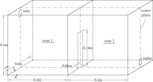
Geometry of the two-zone model room.

Two inlet velocities were chosen: 0.225 and 0.45 m s⁻¹. For an inlet velocity of 0.225 m s⁻¹ air exchange rate (ACH) is 10 h⁻¹. It is understood that the Reynolds number, based on the inlet conditions, is quite low (Re=600), it is the Reynolds number used as a scaling criterion (Posner et al., 2003). Since the key objective of this paper is to validate and apply the drift–flux model, the airflow parameters we selected are not critical. A small chamber with the same dimensions was fabricated. The thickness of the partition wall was ignored in the simulation. The room air was clean at the beginning and particles were supplied at a constant rate with the incoming air. The steady-state airflow characteristics and particle concentration were measured by a phase Doppler Anemometer (Dantec, Denmark). Olive oil droplets generated by an ultrasonic nebulizer (EU-12, Omron, Japan) were used for velocity measurement. For concentration measurement, solid particles were injected with a solid particle disperser (RBG-1000, Palas, Germany), which is able to maintain a stable particle feed rate over a long time period. The concentration of silver-coated hollow glass sphere particles (Dantec) with a nominal diameter of 10 μm was measured by the PDA. A particle passing through the sample volume scatters light that exhibits an angular and temporal intensity distribution characteristic of the particle size and velocity. Particle size and velocity can be determined by analyzing the scattering light with a signal processor. The sample volume has a nominal diameter <100 μm and, therefore, the PDA system is able to achieve point and non-intrusive measurement. The particle number concentration is a derived, not a directly measured, quantity in a PDA measurement. Particle concentration was evaluated with the transit-time-based algorithm as discussed by Hardalupas and Taylor (1989). In order to measure steady-state particle concentration, the fan and particle disperser were switched on for at least 15 min before data acquisition. Each test was conducted three times to give the averaged result.

Fig. 2 shows the velocity field along the center plane. The incoming airflow is blocked by the partition wall and the velocity is very low in the upper part of second zone. Comparisons between the measured and predicted x-direction velocity and particle concentration are shown in Fig. 3, Fig. 4 . Simulation predictions show the same general trends as experimental data and the agreement is quite good, except at points near the floor, where measured velocities are virtually zero. The overall trends of the measured particle concentrations agree with those predicted by the numerical model. Few particles were detected in the second zone of the two-zone chamber. It means that the concentration is nearly zero at these points.

Fig. 2.

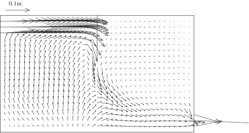
Velocity field in the center plane for inlet velocity 0.225 m s⁻¹. It should be noted that, by default, a vector line starts from numerical grid nodes. It is a display issue that if local velocity is high, velocity vector may extend outside the current zone, but it does not indicate that air can flow through the zone boundary.

Fig. 3.

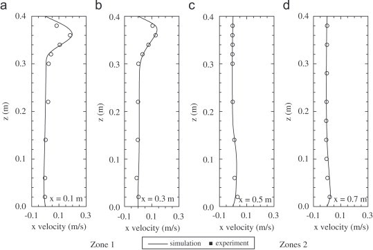
Comparison of measured and predicted x-direction velocity in the two-zone model room (a) x=0.1 m, (b) x=0.3 m, (c) x=0.5 m and (d) x=0.7 m.

Fig. 4.

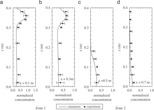
Comparison of measured and predicted concentrations of 10 μm particles in the two-zone model room (a) x=0.1 m, (b) x=0.3 m, (c) x=0.5 m and (d) x=0.7 m.

5. Case study

The previous section shows that the simulation results by the drift–flux model agree very well with the experimental results where a pollutant is released continuously at the inlet. Here we examine a more realistic two-zone scenario where particles are initially released in one zone and subsequently transported to the other zone. Particles are transported to the exposed zone (zone 2) by advection and diffusion processes. Concentrations in zones 1 and 2 are simulated. Both 0.225 and 0.45 m s⁻¹ inlet velocities have been simulated and similar results are observed, so all the results below are based on an inlet velocity of 0.225 m s⁻¹. The particles were assumed to be initially uniformly distributed in zone 1 and the particle concentration is normalized by the initial concentration. Therefore, at t=0, concentrations in zones 1 and 2 are C ₁ ⁺=1 and C ₂ ⁺=0.

6. Results and discussion

Fig. 5(a)–(c) shows the concentration evolution of three particle size groups (0.1, 5 and 10 μm) at various times. The particle concentration level in zone 1 decreases continuously with time elapsed. The concentration near the inlet is very low due to the dilution effect of incoming fresh air. The concentration gradient is less significant below the incoming jet flow. Particles are transported to zone 2 via the partition opening. In the initial phase (time t=0–60 s), concentration in the lower part of zone 2 is higher than that in the upper part. Due to the small vertical air velocity, the dispersion of particles to the upper level is very slow. As observable from the figures, at t=60 s, the concentration in the upper part of zone 2 is almost zero for all of the three particle sizes. However, as concentration in zone 1 deceases to a certain level, the particle concentration in the lower part of zone 2 is diluted by the incoming flow from zone 1. The concentration in the lower part is less than in the upper part. For 0.1 μm particles, it can be observed that at 300 s the concentrations, from the floor up to the height of the opening, are fairly uniform.

Fig. 5.

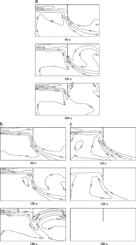
Concentration evolution in the center plane, (a) 0.1 μm; (b) 5 μm; (c) 10 μm for inlet velocity 0.225 m s⁻¹.

Another important observation is that the concentration of large particles is lower than that of small particles due to gravitational settling. For example, the 10 μm particle concentration level decreases rapidly with time, and at 180 s, the particle concentrations are close to zero.

To study exposure in the two zones, Fig. 6, Fig. 7 show the concentration profiles versus time in zones 1 and 2. The concentrations have been measured at breathing height for each zone. The breathing height can be estimated based on the ratio H _b×(H _m/H _r) where H _b, H _m and H _r are breathing height (1.625 m), model room height (0.4 m) and the typical room height (2.5 m), respectively. The locations selected are (x=0.2, y=0.2, z=0.26) and (x=0.6, y=0.2, z=0.26) for zones 1 and 2, respectively. Results obtained by the well-mixed model are depicted for comparison. The concentration level in zone 1 decreases exponentially. At this sampling point (breathing height), the well-mixed model predicts a slower decrease compared to the drift–flux model. Besides the advection process, the overall particle decay rate is augmented by the low vertical mixing rate. It is shown in Fig. 5(a)–(c) that the upward dispersion rate is low and hence at the breathing height, the concentration is low. For the well-mixed model, the concentration in the entire zone is always uniform. For zone 2, the concentration profile at the breathing height increases to reach a peak and then starts to decay. For all particle sizes shown here, there is a very low concentration during the first 60 s at the breathing height. This differs significantly from the well-mixed model prediction. The lag time to reach the peak concentration also varies notably between the two models, 180–240 s for the drift–flux model and 60–180 s for the well-mixed analytical model. The peak concentration levels predicted by the drift–flux simulation are always less than those predicted by the well-mixed model. In summary, due to the underlying homogeneous assumption, the well-mixed model underestimates the breathing height concentration in zone 1 and, more significantly, it severely overestimates the concentration in zone 2 for 0–120 s. The decay rates predicted by the both models also differ. Particles may be trapped in stagnant regions and cannot be removed instantly, so a smaller decay rate is thus predicted. The well-mixed model cannot account for this stagnation phenomenon. One crucial parameter for IAQ assessment is the exposure (or dose). We present the normalized accumulated exposure $({\int }_0^T{C}^{+}\mathrm{d}t)$ versus time for the first 6 min. The accumulated exposures (Fig. 6, Fig. 7) are calculated based on numerical integration of the corresponding concentration profiles as shown in Fig. 6, Fig. 7.

Fig. 6.

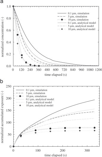
(a) Concentration profiles at the breathing level at zone 1 and (b) accumulated exposure at zone 1.

Fig. 7.

(a) Concentration profiles at the breathing level at zone 2 and (b) accumulated exposure at zone 2.

For zone 1, the initial concentration is maximum but decreases rapidly with time and finally approaches zero. This results in a decreasing exposure rate with time. As expected, the well-mixed model always predicts a lower exposure as compared to the current simulation. Exposure in zone 2 shows very different trend. The initial simulation exposure is low, but the trend is increasing with time. For all particle sizes presented, the predictions by the well-mixed model are always higher than those predicted by the drift–flux simulation. This can be explained by the trend observed in Fig. 6, Fig. 7 in which the exposure predicted by simulation is always higher. By conservation of mass, the accumulated exposure in zone 2 must show the opposite trend as observed in Fig. 6, Fig. 7. For 10 μm particles, the deposition rate is very high and significant loss occurs in zone 1 before advection becomes important. The validity of using a single-point concentration as a surrogate for the entire zone has been discussed by Klepeis (1999). The author suggests that in realistic situations, the well-mixed assumption generally holds, on the condition that the exposure time is much longer than the emission time.

7. Conclusions

A new Eulerian drift–flux model has been applied to simulate particle dispersion and exposure in a two-zone geometry. A phase Doppler Anemometer has been utilized to measure airflow and concentration profiles. Aerosol profiles in a two-zone environment have not been experimentally measured before. Good agreement between the numerical model and the experiment demonstrates that the drift–flux model can be used to predict aerosol deposition and transport in ventilated multi-zone rooms. With the same ventilation rate, the distributions of particles in the two zones are significantly different. Gravity plays a dominant role in the transport of supermicron particles and large supermicron particles which deposit significantly faster than smaller particles. The current drift–flux model predicts that particles are not uniformly distributed in either zone. A well-mixed model based on the mass balance equation was also used to evaluate the profiles of concentration and exposure for the two-zone environment. The well-mixed assumption does not always hold, particularly for supermicron particles. The drift–flux model can be expanded to incorporate more external forces (thermal gradient, surface roughness, etc.) and be further applied to more realistic environments, e.g., furnished rooms with multi-sources.

References

- Beggs C.B., Noakes C.J., Sleigh P.A., Fletcher L.A., Kerr K.G. Methodology for determining the susceptibility of airborne microorganisms to irradiation by an upper-room UVGI system. Journal of Aerosol Science. 2006;37:885–902. [Google Scholar]
- Brown K. Biosecurity: up in the air. Science. 2004;305:1288–1289. doi: 10.1126/science.305.5688.1228. [DOI] [PubMed] [Google Scholar]
- Chang T.-J., Hsieh Y.-F., Kao H.-M. Numerical investigation of airflow pattern and particulate matter transport in naturally ventilated multi-room buildings. Indoor Air. 2006;16:136–152. doi: 10.1111/j.1600-0668.2005.00410.x. [DOI] [PubMed] [Google Scholar]
- Chang T.-J., Kao H.-M., Hsieh Y.-F. Numerical study of ventilation pattern on coarse, fine and very fine particulate matter removal in partitioned indoor environment. Journal of the Air & Waste Management Associations. 2007;57:1189–1700. doi: 10.1080/10473289.2007.10465311. [DOI] [PubMed] [Google Scholar]
- Chen F.Z., Yu S.C.M., Lai A.C.K. Modeling particle distribution and deposition in indoor environments with a new drift–flux model. Atmospheric Environment. 2006;40:357–367. [Google Scholar]
- Chung K.C. Three dimensional analysis of airflow and contaminant particle transport in a partitioned enclosure. Building and Environment. 1999;34:7–17. [Google Scholar]
- Cole E.C., Cook C.E. Characterization of infectious aerosols in health care facilities: an aid to effective engineering controls and preventive strategies. American Journal of Infection Control. 1998;26:453–464. doi: 10.1016/S0196-6553(98)70046-X. [DOI] [PMC free article] [PubMed] [Google Scholar]
- Dols, W.S., Walton, G.N., 2000. CONTANW 2.0 User Manual. MD, National Institute of Standards and Technology.
- Feustel H.E. COMIS—an international multizone air-flow and contaminant transport model. Energy and Buildings. 1999;30:3–18. [Google Scholar]
- FLUENT Inc., 2005. FLUENT 6.2 User's Guide. Lebanon, NH.
- Gadgil A.J., Lobscheid C., Abadie M.O., Finlayson E.U. Indoor pollutant mixing time in an isothermal closed room: an investigation using CFD. Atmospheric Environment. 2003;37:5577–5586. [Google Scholar]
- Gao N.P., Niu J.L. Modeling particle dispersion and deposition in indoor environments. Atmospheric Environment. 2007;41:3862–3876. doi: 10.1016/j.atmosenv.2007.01.016. [DOI] [PMC free article] [PubMed] [Google Scholar]
- Hardalupas Y., Taylor A.M.K.P. On the measurement of particle concentration near a stagnation point. Experiments in Fluids. 1989;8:113–118. [Google Scholar]
- Klepeis N.E. Validity of uniform mixing assumption: determining human exposure to environmental tobacco smoke. Environmental Health Perspectives. 1999;107(Suppl. 2):357–363. doi: 10.1289/ehp.99107s2357. [DOI] [PMC free article] [PubMed] [Google Scholar]
- Lai A.C.K. Particle deposition indoors: A review. Indoor Air. 2002;12:211–214. doi: 10.1034/j.1600-0668.2002.01159.x. [DOI] [PubMed] [Google Scholar]
- Lai A.C.K., Cheng Y.C. Study of expiratory droplet dispersion and transport using a new Eulerian modeling approach. Atmospheric Environment. 2007;41:7473–7484. doi: 10.1016/j.atmosenv.2007.05.045. [DOI] [PMC free article] [PubMed] [Google Scholar]
- Lai A.C.K., Nazaroff W.W. Modeling indoor particle deposition from turbulent flow onto smooth surfaces. Journal of Aerosol Science. 2000;31:463–476. [Google Scholar]
- Li Y., Huang X., Yu I.T.S., Wong T.W., Qian H. Role of air distribution in SARS transmission during the largest nosocomial outbreak in Hong Kong. Indoor Air. 2005;15:83–95. doi: 10.1111/j.1600-0668.2004.00317.x. [DOI] [PubMed] [Google Scholar]
- Li Y., Leung G.M., Tang J.W., Yang X., Chao C.Y.H., Lin J.Z., Lu J.W., Nielsen P.V., Niu J., Qian H., Sleigh A.C., Su H.-J.J., Sundell J., Wong T.W., Yuen P.L. Role of ventilation in airborne transmission of infectious agents in the built environment—a multidisciplinary systematic review. Indoor Air. 2007;17:2–18. doi: 10.1111/j.1600-0668.2006.00445.x. [DOI] [PubMed] [Google Scholar]
- Mangili A., Gendreau M.A. Transmission of infectious diseases during commercial air travel. Lancet. 2005;365:989–996. doi: 10.1016/S0140-6736(05)71089-8. [DOI] [PMC free article] [PubMed] [Google Scholar]
- Miller S.L., Nazaroff W.W. Environmental tobacco smoke particles in multizone indoor environments. Atmospheric Environment. 2001;35:2053–2067. [Google Scholar]
- Nardell E.A. The role of ventilation in preventing nosocomial transmission of tuberculosis. International Journal of Tuberculosis and Lung Diseases. 1998;2:S110–S117. [PubMed] [Google Scholar]
- Nicas M., Nazaroff W.W., Hubbard A. Toward understanding the risk of secondary airborne infection: emission of respirable pathogens. Journal of Occupational and Environmental Hygiene. 2005;2:143–154. doi: 10.1080/15459620590918466. [DOI] [PMC free article] [PubMed] [Google Scholar]
- Posner J.D., Buchanan C.R., Dunn-Rankin D. Measurement and prediction of indoor air flow in a model room. Energy and Buildings. 2003;35:515–526. [Google Scholar]
- Richmond-Bryant J., Eisner A.D., Brixey L.A., Wiener R.W. Transport of airborne particles within a room. Indoor Air. 2006;16:48–55. doi: 10.1111/j.1600-0668.2005.00398.x. [DOI] [PubMed] [Google Scholar]
- Wan M.P., Chao C.Y.H., Ng Y.D., Sze To G.N., Yu W.C. Dispersion of expiratory aerosols in a general hospital ward with ceiling mixing type mechanical ventilation system. Aerosol Science and Technology. 2007;41:244–258. [Google Scholar]
- Wang J.B., Lai A.C.K. A new drift–flux model for particle transport and deposition in human airways. Journal of Biomechanical Engineering. 2006;128:97–105. doi: 10.1115/1.2133763. [DOI] [PubMed] [Google Scholar]
- Weichenthal S., Dufresne A., Infante-Rivard C. Indoor ultrafine particles and childhood asthma: exploring a potential public health concern. Indoor Air. 2007;17:81–91. doi: 10.1111/j.1600-0668.2006.00446.x. [DOI] [PubMed] [Google Scholar]
- Williams R., Creason J., Zweidinger R., Watts R., Sheldon L., Shy C. Indoor, outdoor, and personal exposure monitoring of particulate air pollution: the Baltimore elderly epidemiology—exposure pilot study. Atmospheric Environment. 2000;34:4193–4204. [Google Scholar]
- Zhang Z., Chen Q. Experimental measurements and numerical simulations of particle transport and distribution in ventilated rooms. Atmospheric Environment. 2006;40:3396–3408. [Google Scholar]
- Zhao B., Wu J. Modeling particle deposition from fully developed turbulent flow in ventilation duct. Atmospheric Environment. 2006;40:457–466. [Google Scholar]
- Zhao B., Zhang Y., Li X.T., Yang X.D., Huang D.T. Comparison of indoor aerosol particle concentration and deposition in different ventilated rooms by numerical method. Building and Environment. 2004;39:1–8. [Google Scholar]