Numerical study of SARS epidemic model with the inclusion of diffusion in the system

Abstract

This paper deals with the numerical study of population model based on the epidemics of Severe Acute Respiratory Syndrome (SARS). SEIJR (susceptible, exposed, infected, diagnosed, recovered) model of SARS epidemic is considered with net in flow of individuals into a region. Transmission of disease is analyzed by solving the system of differential equations using numerical methods with different initial population distributions. The effect of diffusion on the spread of disease is examined. Stability is established for the numerical solutions. Effects of interventions (medical and non medical) are also analyzed.

1. Introduction

Epidemiological models are considered as one of the most powerful tools to analyze and understand the spread and control of infectious diseases. Analysis of transmission dynamics of infectious diseases can lead to the better methodologies to slow their transmission. Since the start of twentieth century, a lot of work has been done on construction of epidemic models for infectious diseases such as chicken pox, diphtheria, gonorrhea, influenza, malaria, rabies, rubella, whooping cough and SARS. Models have also been developed for sexually transmitted diseases like syphilis, $\mathit{HIV}/\mathit{AIDS}$, and child diseases like measles and polio. These models ranges from simple curve fitting models to standard compartmental models [1] ($\mathit{MSEIR}\text{,}\mathit{MSEIRS}\text{,}\mathit{SEIJR}\text{,}\mathit{SIR}\text{,}\mathit{SIRS}$, $\mathit{SEIR}\text{,}\mathit{SEIS}\text{,}\mathit{SI}$, and SIS etc.) to complex stochastic models. Fast computer systems and the availability of huge data bases has made it possible to use complex mathematical models to analyze the data.

Daniel Bernoulli is considered to be the first who tried to evaluate the effectiveness of vaccination on healthy people with the smallpox virus in 1690. In 1906, Hamer constructed and analyzed a discrete time model in order to understand the reoccurrence of measles epidemics. His model was probably the first to assume that the incidence (number of new cases per unit time) depends on the product of the densities of the susceptibles and infectives [9]. Ross [9] was interested in the prevalence and control of malaria and he developed deterministic model for malaria as a host-vector disease in 1911. Other deterministic epidemiological models were then developed by Ross, Ross and Hudson, Martini and Lotka [9]. Kermack and McKendrick are considered as the pioneers in mathematical modeling in epidemiology with the publication of a series of papers in 1926. In their work they calculated the epidemic threshold and showed that an outbreak of an epidemic could occur only if the number of susceptible individuals exceed the critical value called the reproduction number. Mathematical epidemiology seems to have grown rapidly since then as a large variety of models have been formulated, mathematically analyzed and applied to infectious diseases [9]. The first edition of Bailey’s book, which appeared in 1957, is an important landmark in the history of mathematical biology [9].

Severe Acute Respiratory Syndrome (SARS) is one of the recently emerged infectious diseases. This is a viral respiratory illness caused by a coronavirus, called SARS-associated coronavirus ($\mathit{SARS}$–$\mathit{CoV}$). It was in November 2002, when the first case of SARS was diagnosed in the Chinese province of Guangdong. At the end of February 2003, the SARS epidemic spread around the world, when a medical doctor from Guangdong infected several persons in a hotel in Kowloon. SARS also spread globally through air travel. According to the estimates of $\mathit{WHO}\text{,}8450$ people were infected and 810 deaths were recorded due to SARS in 33 countries on 5 continents [15]. Although this outbreak of the disease was brought under control at the end of 2003, many separate outbreaks of SARS appeared in Singapore, Taiwan and China. The main reason for this was the release of $\mathit{SARS}$–$\mathit{CoV}$ accidently from laboratories [15]. The animals infected by the $\mathit{SARS}$–$\mathit{CoV}$ strain also infected humans and at the start of 2004 some new cases of this disease came to notice. Both incidents show the danger of SARS outbreak at any time in the near future, either by $\mathit{SARS}$–$\mathit{CoV}$ virus evolving from $\mathit{SARS}$–$\mathit{CoV}$-like virus from animals or by virus from laboratory samples. There is a $\mathit{SARS}$–$\mathit{CoV}$-like virus, also found in animals, but it is not transferable and thus cannot cause SARS-like disease. It is possible that under special circumstances, this virus may get converted into the early human $\mathit{SARS}$–$\mathit{CoV}$, with an ability to transfer from animals to humans [8].

A large number of papers appeared in the literature on infectious disease SARS in 2003. In the beginning, epidemiologist, tried to find out the reasons for the cause and spread of SARS. They tried to find measures to control it, but the main emphasis was on research work concerned with the biological properties of the corona virus [16]. Some work was done to investigate the transmission dynamics and the effect of various control measures. Most of the study on SARS was done in China, where the SARS epidemic hit the hardest. This work was published in Chinese journals, which were poorly accessible to international researchers. Xia et al. [17] analyzed the pattern of SARS and predicted the course of the SARS epidemic by establishing a compartmental model using data from Guangdong and Hong Kong. Chowell et al. [5] fitted an SEIJR model for SARS epidemic for the data from Toronto, Hong Kong and Singapore. Chowell predicted the behavior of the disease and the role of diagnosis and isolation as a control mechanism in these regions showing the difference between the epidemic dynamics occurred in these three cities. Yang et al. [19] established a compartmental model to describe the SARS epidemic in spatial–temporal dimensions determining whether people traveling in buses and trains infect one another or not. They concluded that SARS can spread through people traveling in buses and trains. In their SEIR models based on data from Beijing and Hong Kong, Wu et al. [14] and Chen et al. [4] estimated the source of super-spreading events of SARS with the calculation of the reproductive rate of the disease based on data from Beijing and Hong Kong.

In this paper, a SARS model (Chowell et al. [5]) is considered with the inclusion of diffusion in the system. The diffusion is introduced in the system to study the spacial spread of disease. Different initial population distributions are chosen to investigate the effect of diffusion on the spread of SARS. Also intervention strategies have been proposed to investigate the effect on spread of disease.

2. The SEIJR epidemic model

2.1. Equations

This model is based on the SEIJR model (Chowell et al. [5]) with the inclusion of diffusion in the equations governing the system. Total population is supposed to be N where $N=S+E+I+J+R$.

$$\frac{\partial S}{\partial t}=-\beta \frac{(I+\mathit{qE}+\mathit{lJ})}{N}S-\mu S+\mathrm{\Pi }+d_1\frac{{\partial }^{2}S}{\partial x^2}\text{,}$$ (1)

$$\frac{\partial E}{\partial t}=\beta \frac{(I+\mathit{qE}+\mathit{lJ})}{N}S-(\mu +\kappa )E+d_2\frac{{\partial }^{2}E}{\partial x^2}\text{,}$$ (2)

$$\frac{\partial I}{\partial t}=\kappa E-(\mu +\alpha +{\gamma }_1+\delta )I+d_3\frac{{\partial }^{2}I}{\partial x^2}\text{,}$$ (3)

$$\frac{\partial J}{\partial t}=\alpha I-(\mu +{\gamma }_2+\delta )J+d_4\frac{{\partial }^{2}J}{\partial x^2}\text{,}$$ (4)

$$\frac{\partial R}{\partial t}={\gamma }_{1}I+{\gamma }_{2}J-\mu R+d_5\frac{{\partial }^{2}R}{\partial x^2}\text{,}$$ (5)

where the variables $S\text{,}E\text{,}I\text{,}J$ and R denote the proportion of susceptible, exposed, infected, diagnosed and recovered individuals respectively. $d_1\text{,}{d}_2\text{,}{d}_3\text{,}{d}_4$ and $d_5$ are the diffusivity constants. Table 1 provides the description and the values of the parameters.

Table 1.

Interpretation of parameters (per day).

Parameter	Description	Values
$\mathrm{\Pi }$	Rate of inflow of susceptible individuals into region	$3.3\times {10}^{-5}$b
$\beta$	Transmission Rate	$0.75$a
$\mu$	Rate of natural mortality	$3.4\times {10}^{-5}$b
l	Relative measure of reduced risk among diagnosed	$0.38$a
$\kappa$	Rate of progression from exposed to the infectives	$0.33$a
q	Relative measure of infectiousness for exposed individuals	$0.1$a
$\alpha$	Rate of progression from infective to diagnosed	$0.33$a
${\gamma }_1$	recovery rate of infected individuals	$0.125$a
${\gamma }_2$	recovery rate of diagnosed individuals	$0.2$a
$\delta$	SARS induced mortality rate	$0.006$a

^aChowell et al. [5]

^bGummel et al. [10]

2.2. Initial and boundary conditions

The domain of all the calculations is considered as $[-2\text{,}2]$. Boundary and initial conditions are chosen as follows:

$$\frac{\partial S(-2\text{,}t)}{\partial x}=\frac{\partial E(-2\text{,}t)}{\partial x}=\frac{\partial I(-2\text{,}t)}{\partial x}=\frac{\partial J(-2\text{,}t)}{\partial x}=\frac{\partial R(-2\text{,}t)}{\partial x}=0\text{,}$$ (6)

$$\frac{\partial S(2\text{,}t)}{\partial x}=\frac{\partial E(2\text{,}t)}{\partial x}=\frac{\partial I(2\text{,}t)}{\partial x}=\frac{\partial J(2\text{,}t)}{\partial x}=\frac{\partial R(2\text{,}t)}{\partial x}=0\text{,}$$ (7)

• 1.
  $$\begin{array}{cc}\hfill & S_0=0.98\mathit{Sech}(5x-1)\text{,}-2⩽x⩽2\text{.}\hfill \\ \hfill & E_0=0\text{,}-2⩽x⩽2\text{.}\hfill \\ \hfill & I_0=0.02\mathit{Sech}(5x-1)\text{,}-2⩽x⩽2\text{.}\hfill \\ \hfill & J_0=0\text{,}-2⩽x⩽2\text{.}\hfill \\ \hfill & R_0=0\text{,}-2⩽x⩽2\text{.}\hfill \end{array}$$
• 2.
  $$\begin{array}{cc}\hfill & S_0=0.98\mathit{exp}{(-5x^2)}^3\text{,}-2⩽x⩽2\text{.}\hfill \\ \hfill & E_0=0\text{,}-2⩽x⩽2\text{.}\hfill \\ \hfill & I_0=\left\{\begin{array}{cc}0\text{,}\hfill & -2⩽x<-0.4\text{,}\hfill \\ 0.02\text{,}\hfill & -0.4⩽x⩽0.4\text{,}\hfill \\ 0\text{,}\hfill & 0.4<x\le 2\text{.}\hfill \end{array}\right)\hfill \\ \hfill & J_0=0\text{,}-2⩽x⩽2\text{.}\hfill \\ \hfill & R_0=0\text{,}-2⩽x⩽2\text{.}\hfill \end{array}$$
• 3.
  $$\begin{array}{cc}\hfill & S_0=0.97\mathit{exp}(-5{(x-1)}^2)\text{,}-2⩽x⩽2\text{.}\hfill \\ \hfill & E_0=0\text{,}-2⩽x⩽2\text{.}\hfill \\ \hfill & I_0=0.03\mathit{exp}(-5{(x+1)}^2)\text{,}-2⩽x⩽2\text{.}\hfill \\ \hfill & J_0=0\text{,}-2⩽x⩽2\text{.}\hfill \\ \hfill & R_0=0\text{,}-2⩽x⩽2\text{.}\hfill \end{array}$$
• 4.
  $$\begin{array}{cc}\hfill & S_0=\left\{\begin{array}{cc}0.96\mathit{Sech}(15x)\text{,}\hfill & -2⩽x⩽0\text{,}\hfill \\ 0\text{,}\hfill & 0<x⩽2\text{.}\hfill \end{array}\right)\hfill \\ \hfill & E_0=0\text{,}-2⩽x⩽-5\text{.}\hfill \\ \hfill & I_0=\left\{\begin{array}{cc}0\text{,}\hfill & -2⩽x<-0.6\text{,}\hfill \\ 0.04\text{,}\hfill & -0.6⩽x⩽0.6\text{,}\hfill \\ 0\text{,}\hfill & 0.6<x⩽2\text{.}\hfill \end{array}\right)\hfill \\ \hfill & J_0=0\text{,}-2⩽x⩽2\text{.}\hfill \\ \hfill & R_0=0\text{,}-2⩽x⩽2\text{.}\hfill \end{array}$$

The initial conditions are shown in Fig. 1 . In initial condition $(i)$ a large proportion of susceptible and infected populations is concentrated towards the right half of the main domain. Initial condition $(\mathit{ii})$ shows both S and I concentrated around the middle of the main domain. In initial condition $(\mathit{iii})\text{,}I$ has high concentration in the left half of the domain $[-2\text{,}2]$ and population S has concentration on the right half of the domain $[-2\text{,}2]$. Initial condition $(\mathit{iv})$ shows susceptible S around the middle of domain $[-2\text{,}2]$ and infectious individuals around the middle but beyond the domain of S.

Fig. 1.

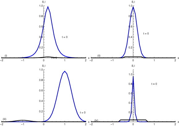
Initial conditions $(i)$–$(\mathit{iv})$.

3. Numerical scheme

In this section the operator splitting technique [18] has been used to solve the SEIJR model equations. The equations are divided in two groups of sub equations. The first group comprises the nonlinear reaction equations to be used for the first half-time step as given:

$$\frac{1}{2}\frac{\partial S}{\partial t}=-\beta \frac{(I+\mathit{qE}+\mathit{lJ})}{N}S-\mu S+\mathrm{\Pi }\text{,}$$ (8)

$$\frac{1}{2}\frac{\partial E}{\partial t}=\beta \frac{(I+\mathit{qE}+\mathit{lJ})}{N}S-(\mu +\kappa )E\text{,}$$ (9)

$$\frac{1}{2}\frac{\partial I}{\partial t}=\kappa E-(\mu +\alpha +{\gamma }_1+\delta )I\text{,}$$ (10)

$$\frac{1}{2}\frac{\partial J}{\partial t}=\alpha I-(\mu +{\gamma }_2+\delta )J\text{,}$$ (11)

$$\frac{1}{2}\frac{\partial R}{\partial t}={\gamma }_{1}I+{\gamma }_{2}J-\mu R\text{,}$$ (12)

The second group consists of the linear diffusion equations, to be used for the second half-time step as follows:

$$\frac{1}{2}\frac{\partial S}{\partial t}=d_1\frac{{\partial }^{2}S}{\partial x^2}\text{,}$$ (13)

$$\frac{1}{2}\frac{\partial E}{\partial t}=d_2\frac{{\partial }^{2}E}{\partial x^2}\text{,}$$ (14)

$$\frac{1}{2}\frac{\partial I}{\partial t}=d_3\frac{{\partial }^{2}I}{\partial x^2}\text{,}$$ (15)

$$\frac{1}{2}\frac{\partial J}{\partial t}=d_4\frac{{\partial }^{2}R}{\partial x^2}\text{,}$$ (16)

$$\frac{1}{2}\frac{\partial R}{\partial t}=d_5\frac{{\partial }^{2}R}{\partial x^2\text{,}}$$ (17)

By the forward Euler scheme the above equations transform to

$$S_i^{j+\frac{1}{2}}=S_i^j+\mathrm{\Delta }t\left(-\beta \frac{(I_i^j+{\mathit{qE}}_i^j+{\mathit{lJ}}_i^j)}{N_i^j}{S}_i^j-\mu S_i^j+\mathrm{\Pi }\right)\text{,}$$ (18)

$$E_i^{j+\frac{1}{2}}=E_i^j+\mathrm{\Delta }t\left(\beta \frac{(I_i^j+{\mathit{qE}}_i^j+{\mathit{lJ}}_i^j)}{N_i^j}{S}_i^j-(\mu +\kappa )E_i^j\right)\text{,}$$ (19)

$$I_i^{j+\frac{1}{2}}=I_i^j+\mathrm{\Delta }t(\kappa E_i^j-(\mu +\alpha +{\gamma }_1+\delta )I_i^j)\text{,}$$ (20)

$$J_i^{j+\frac{1}{2}}=J_i^j+\mathrm{\Delta }t(\alpha I_i^j-(\mu +{\gamma }_2+\delta )J_i^j)\text{,}$$ (21)

$$R_i^{j+\frac{1}{2}}=R_i^j+\mathrm{\Delta }t({\gamma }_1{I}_i^j+{\gamma }_2{J}_i^j-\mu R_i^j)\text{,}$$ (22)

where $S_i^j\text{,}{E}_i^j\text{,}{I}_i^j\text{,}{J}_i^j$ and $R_i^j$ are the approximated values of $S\text{,}E\text{,}I\text{,}J$ and R at position $-2+i\mathrm{\Delta }x$, for $i=0\text{,}1\text{,}\dots$ and time $j\mathrm{\Delta }t\text{,}j=0\text{,}1\text{,}\dots$ and $S_i^{j+\frac{1}{2}}\text{,}{E}_i^{j+\frac{1}{2}}\text{,}{I}_i^{j+\frac{1}{2}}\text{,}{J}_i^{j+\frac{1}{2}}$, and $R_i^{j+\frac{1}{2}}$ denote their values at the first half-time step. Similarly, for the second half-time step,

$$S_i^{j+1}=S_i^{j+\frac{1}{2}}+d_1\frac{\mathrm{\Delta }t}{{(\mathrm{\Delta }x)}^2}\left(S_{i-1}^{j+\frac{1}{2}}-2S_i^{j+\frac{1}{2}}+S_{i+1}^{j+\frac{1}{2}}\right)\text{,}$$ (23)

$$E_i^{j+1}=E_i^{j+\frac{1}{2}}+d_2\frac{\mathrm{\Delta }t}{{(\mathrm{\Delta }x)}^2}\left(E_{i-1}^{j+\frac{1}{2}}-2E_i^{j+\frac{1}{2}}+E_{i+1}^{j+\frac{1}{2}}\right)\text{,}$$ (24)

$$I_i^{j+1}=I_i^{j+\frac{1}{2}}+d_3\frac{\mathrm{\Delta }t}{{(\mathrm{\Delta }x)}^2}\left(I_{i-1}^{j+\frac{1}{2}}-2I_i^{j+\frac{1}{2}}+I_{i+1}^{j+\frac{1}{2}}\right)\text{,}$$ (25)

$$J_i^{j+1}=J_i^{j+\frac{1}{2}}+d_4\frac{\mathrm{\Delta }t}{{(\mathrm{\Delta }x)}^2}\left(J_{i-1}^{j+\frac{1}{2}}-2J_i^{j+\frac{1}{2}}+J_{i+1}^{j+\frac{1}{2}}\right)\text{,}$$ (26)

$$R_i^{j+1}=R_i^{j+\frac{1}{2}}+d_5\frac{\mathrm{\Delta }t}{{(\mathrm{\Delta }x)}^2}\left(R_{i-1}^{j+\frac{1}{2}}-2R_i^{j+\frac{1}{2}}+R_{i+1}^{j+\frac{1}{2}}\right)\text{.}$$ (27)

The stability condition satisfied by the above described numerical method is given as:

$$\frac{d_n\mathrm{\Delta }t}{{(\mathrm{\Delta }x)}^2}⩽0.5\text{,}n=1\text{,}2\text{,}3\text{,}4\text{,}5\text{.}$$ (28)

In each case, $\mathrm{\Delta }x=0.1\text{,}{d}_1=0.025\text{,}{d}_2=0.01\text{,}{d}_3=0.001\text{,}{d}_4=0.0\text{,}{d}_5=0.0$ and $\mathrm{\Delta }t=0.03$ are used.

3.1. Disease-free equilibrium $(\mathit{DFE})$ and stability analysis

The threshold parameter for any DFE is ${\mathfrak{R}}_0$, referred to as the basic reproduction number. It is defined as “the expected number of secondary cases produced, in a completely susceptible population, by a typical infective individual [6]. The variational matrix of the system of Eqs. (1), (2), (3), (4), (5) at the disease-free equilibrium $P_0=(1\text{,}0\text{,}0\text{,}0\text{,}0)$, is calculated using the same technique as [7] and given as follows:

$$V^0=\left[\begin{array}{ccccc}\hfill -\mu \hfill & \hfill -q\beta \hfill & \hfill -\beta \hfill & \hfill -l\beta \hfill & \hfill 0\hfill \\ \hfill 0\hfill & \hfill q\beta -\kappa -\mu \hfill & \hfill \beta \hfill & \hfill l\beta \hfill & \hfill 0\hfill \\ \hfill 0\hfill & \hfill \kappa \hfill & \hfill -\mu -\alpha -{\gamma }_1-\delta \hfill & \hfill 0\hfill & \hfill 0\hfill \\ \hfill 0\hfill & \hfill 0\hfill & \hfill \alpha \hfill & \hfill -\mu -{\gamma }_2-\delta \hfill & \hfill 0\hfill \\ \hfill 0\hfill & \hfill 0\hfill & \hfill {\gamma }_1\hfill & \hfill {\gamma }_2\hfill & \hfill -\mu \hfill \end{array}\right]$$

Trace$[V^0]=q\beta -(5\mu +\alpha +\kappa +{\gamma }_1+{\gamma }_2+\delta )<0$, for $\beta <\frac{5\mu +\alpha +\kappa +{\gamma }_1+{\gamma }_2+\delta }{q}$Det$[V^0]=(l\alpha \beta \kappa +\beta \kappa (\mu +{\gamma }_2+\delta )+(\mu +\alpha +{\gamma }_1+\delta )(\mu +{\gamma }_2+\delta )(q\beta -\mu -\kappa )){\mu }^2>0$, for ${\mathfrak{R}}_0<1$, where ${\mathfrak{R}}_0=\frac{q(\mu +\alpha +{\gamma }_1+\delta )(\mu +{\gamma }_2+\delta )+\kappa (\mu +{\gamma }_2+\delta )+l\alpha \kappa }{(\mu +\alpha +{\gamma }_1+\delta )(\mu +{\gamma }_2+\delta )(\kappa +\mu )}$.

This shows that $P_0$ is stable for ${\mathfrak{R}}_0<1$. In the same way we can illustrate the stability of the endemic point for ${\mathfrak{R}}_0>1$.

3.2. Stability of endemic equilibrium without diffusion

The variational matrix of the system of Eqs. (1), (2), (3), (4), (5) at $P^{\ast }(S^{\ast }\text{,}{E}^{\ast }\text{,}{I}^{\ast }\text{,}{J}^{\ast }{R}^{\ast })$, is given by

$$V^{\ast }=\left[\begin{array}{ccccc}\hfill a_{11}\hfill & \hfill a_{12}\hfill & \hfill a_{13}\hfill & \hfill a_{14}\hfill & \hfill a_{15}\hfill \\ \hfill a_{21}\hfill & \hfill a_{22}\hfill & \hfill a_{23}\hfill & \hfill a_{24}\hfill & \hfill a_{25}\hfill \\ \hfill a_{31}\hfill & \hfill a_{32}\hfill & \hfill a_{33}\hfill & \hfill a_{34}\hfill & \hfill a_{35}\hfill \\ \hfill a_{41}\hfill & \hfill a_{42}\hfill & \hfill a_{43}\hfill & \hfill a_{44}\hfill & \hfill a_{45}\hfill \\ \hfill a_{51}\hfill & \hfill a_{52}\hfill & \hfill a_{53}\hfill & \hfill a_{54}\hfill & \hfill a_{55}\hfill \end{array}\right]\text{,}$$

where

$$a_{11}=\beta \frac{(I^{\ast }+{\mathit{qE}}^{\ast }+{\mathit{lJ}}^{\ast })S^{\ast }}{{(S^{\ast }+E^{\ast }+I^{\ast }+J^{\ast }+R^{\ast })}^2}-\beta \frac{(I^{\ast }+{\mathit{qE}}^{\ast }+{\mathit{lJ}}^{\ast })}{(S^{\ast }+E^{\ast }+I^{\ast }+J^{\ast }+R^{\ast })}-\mu \text{,}$$

$$a_{12}=\beta \frac{(I^{\ast }+{\mathit{qE}}^{\ast }+{\mathit{lJ}}^{\ast })S^{\ast }}{{(S^{\ast }+E^{\ast }+I^{\ast }+J^{\ast }+R^{\ast })}^2}-\beta \frac{{\mathit{qS}}^{\ast }}{(S^{\ast }+E^{\ast }+I^{\ast }+J^{\ast }+R^{\ast })}\text{,}$$

$$a_{13}=\beta \frac{(I^{\ast }+{\mathit{qE}}^{\ast }+{\mathit{lJ}}^{\ast })S^{\ast }}{{(S^{\ast }+E^{\ast }+I^{\ast }+J^{\ast }+R^{\ast })}^2}-\beta \frac{S^{\ast }}{(S^{\ast }+E^{\ast }+I^{\ast }+J^{\ast }+R^{\ast })}\text{,}$$

$$a_{14}=\beta \frac{(I^{\ast }+{\mathit{qE}}^{\ast }+{\mathit{lJ}}^{\ast })S^{\ast }}{{(S^{\ast }+E^{\ast }+I^{\ast }+J^{\ast }+R^{\ast })}^2}-\beta \frac{{\mathit{lS}}^{\ast }}{(S^{\ast }+E^{\ast }+I^{\ast }+J^{\ast }+R^{\ast })}\text{,}$$

$$a_{21}=\beta \frac{1}{(S^{\ast }+E^{\ast }+I^{\ast }+J^{\ast }+R^{\ast })}-\beta \frac{(I^{\ast }+{\mathit{qE}}^{\ast }+{\mathit{lJ}}^{\ast })S^{\ast }}{{(S^{\ast }+E^{\ast }+I^{\ast }+J^{\ast }+R^{\ast })}^2}\text{,}$$

$$a_{22}=\beta \frac{{\mathit{qS}}^{\ast }}{(S^{\ast }+E^{\ast }+I^{\ast }+J^{\ast }+R^{\ast })}-\beta \frac{(I^{\ast }+{\mathit{qE}}^{\ast }+{\mathit{lJ}}^{\ast })S^{\ast }}{{(S^{\ast }+E^{\ast }+I^{\ast }+J^{\ast }+R^{\ast })}^2}-\kappa -\mu \text{,}$$

$$a_{23}=\beta \frac{S^{\ast }}{(S^{\ast }+E^{\ast }+I^{\ast }+J^{\ast }+R^{\ast })}-\beta \frac{(I^{\ast }+{\mathit{qE}}^{\ast }+{\mathit{lJ}}^{\ast })S^{\ast }}{{(S^{\ast }+E^{\ast }+I^{\ast }+J^{\ast }+R^{\ast })}^2}\text{,}$$

$$a_{24}=\beta \frac{{\mathit{lS}}^{\ast }}{(S^{\ast }+E^{\ast }+I^{\ast }+J^{\ast }+R^{\ast })}-\beta \frac{(I^{\ast }+{\mathit{qE}}^{\ast }+{\mathit{lJ}}^{\ast })S^{\ast }}{{(S^{\ast }+E^{\ast }+I^{\ast }+J^{\ast }+R^{\ast })}^2}\text{,}$$

$$a_{15}=\beta \frac{(I^{\ast }+{\mathit{qE}}^{\ast }+{\mathit{lJ}}^{\ast })S^{\ast }}{{(S^{\ast }+E^{\ast }+I^{\ast }+J^{\ast }+R^{\ast })}^2}\text{,}{a}_{25}=-\beta \frac{(I^{\ast }+{\mathit{qE}}^{\ast }+{\mathit{lJ}}^{\ast })S^{\ast }}{{(S^{\ast }+E^{\ast }+I^{\ast }+J^{\ast }+R^{\ast })}^2}\text{,}$$

$$a_{32}=\kappa \text{,}{a}_{33}=-\alpha -{\gamma }_1-\delta -\mu \text{,}{a}_{43}=\alpha \text{,}{a}_{44}=-{\gamma }_2-\delta -\mu \text{,}{a}_{53}={\gamma }_1\text{,}$$

$a_{54}={\gamma }_2$, $a_{55}=-\mu$, and $a_{31}=$ $a_{34}=$ $a_{35}=$ $a_{41}=$ $a_{42}=$ $a_{45}=$ $a_{51}=$ $a_{52}=0$. The characteristic equation for $P^{\ast }(S^{\ast }\text{,}{E}^{\ast }\text{,}{I}^{\ast }\text{,}{J}^{\ast }\text{,}{R}^{\ast })$ can be written as

$${\lambda }^5+p_1{\lambda }^4+p_2{\lambda }^3+p_3{\lambda }^2+p_4\lambda +p_5=0\text{.}$$ (29)

Where $p_1\text{,}{p}_2\text{,}{p}_3\text{,}{p}_4$ and $p_5$ are calculated as in [12].

The Routh–Hurwitz criterion for the stability is given as in [13]:

$C_1:p_1>0\text{,}{p}_5>0$,

$C_2:p_1{p}_2>p_3$,

$C_3:p_1{p}_2{p}_3+p_1{p}_5>p_3^2+p_1^2{p}_4$,

$C_4:(p_1{p}_4-p_5)(p_1{p}_2{p}_3-p_3^2-p_1^2{p}_4)+p_1^2{p}_4{p}_5>p_5{(p_1{p}_2-p_3)}^2+p_1{p}_5^2$. and $P_1\text{,}{P}_2\text{,}{P}_3$ and $P_4$ are points of equilibrium.

$P1=(.331581\text{,}0.000064\text{,}0.000046\text{,}0.000074\text{,}.607887)$,

$P2=(.357187\text{,}.000062\text{,}.000044\text{,}.000058\text{,}.585632)$,

$P3=(.365393\text{,}.000061\text{,}.000039\text{,}.000064\text{,}.577199)$,

$P4=(.355572\text{,}.000062\text{,}.000044\text{,}.000072\text{,}.584715)$.

3.3. Stability of endemic equilibrium with diffusion

To calculate the small perturbations $S_1(x\text{,}t)\text{,}{E}_1(x\text{,}t)\text{,}{I}_1(x\text{,}t)\text{,}{J}_1(x\text{,}t)$ and $R_1(x\text{,}t)$, the equations are linearized about the point of equilibrium $P^{\ast }(S^{\ast }\text{,}{E}^{\ast }\text{,}{I}^{\ast }\text{,}{J}^{\ast }\text{,}{R}^{\ast })$ as described in [2], [11].

$$\frac{\partial S_1}{\partial t}=a_{11}{S}_1+a_{12}{E}_1+a_{13}{I}_1+a_{14}{J}_1+a_{15}{R}_1+d_1\frac{{\partial }^2{S}_1}{\partial x^2}\text{,}$$ (30)

$$\frac{\partial E_1}{\partial t}=a_{21}{S}_1+a_{22}{E}_1+a_{23}{I}_1+a_{24}{J}_1+a_{25}{R}_1+d_2\frac{{\partial }^2{E}_1}{\partial x^2}\text{,}$$ (31)

$$\frac{\partial I_1}{\partial t}=a_{31}{S}_1+a_{32}{E}_1+a_{33}{I}_1+a_{34}{J}_1+a_{35}{R}_1+d_3\frac{{\partial }^2{I}_1}{\partial x^2}\text{,}$$ (32)

$$\frac{\partial J_1}{\partial t}=a_{41}{S}_1+a_{42}{E}_1+a_{43}{I}_1+a_{44}{J}_1+a_{45}{R}_1+d_4\frac{{\partial }^2{J}_1}{\partial x^2}\text{,}$$ (33)

$$\frac{\partial R_1}{\partial t}=a_{51}{S}_1+a_{52}{E}_1+a_{53}{I}_1+a_{54}{J}_1+a_{55}{R}_1+d_5\frac{{\partial }^2{R}_1}{\partial x^2}\text{,}$$ (34)

where $a_{11}\text{,}{a}_{12}\text{,}{a}_{13}$ etc. are the elements of the variational matrix $V^{\ast }$ calculated using same method as described in [12]. Assume a Fourier series solution exists of Eqs. (30), (31), (32), (33), (34) of the form:

$$S_1(x\text{,}t)={\displaystyle \sum _k}{S}_k{e}^{\lambda t}\mathit{cos}(\mathit{kx})\text{,}$$ (35)

$$E_1(x\text{,}t)={\displaystyle \sum _k}{E}_k{e}^{\lambda t}\mathit{cos}(\mathit{kx})\text{,}$$ (36)

$$I_1(x\text{,}t)={\displaystyle \sum _k}{I}_k{e}^{\lambda t}\mathit{cos}(\mathit{kx})\text{,}$$ (37)

$$J_1(x\text{,}t)={\displaystyle \sum _k}{J}_k{e}^{\lambda t}\mathit{cos}(\mathit{kx})\text{,}$$ (38)

$$R_1(x\text{,}t)={\displaystyle \sum _k}{R}_k{e}^{\lambda t}\mathit{cos}(\mathit{kx})\text{,}$$ (39)

where $k=\frac{n\pi }{2}\text{,}(n=1\text{,}2\text{,}3\text{,}\dots )$ is the wave number for the node n. Substituting the value of $S_1\text{,}{E}_1$, $I_1\text{,}{R}_1$ in Eqs. (30), (31), (32), (33), (34), the equations are transformed into

$${\displaystyle \sum _k}(a_{11}-d_1{k}^2-\lambda )S_k+{\displaystyle \sum _k}{a}_{12}{E}_k+{\displaystyle \sum _k}{a}_{13}{I}_k++{\displaystyle \sum _k}{a}_{14}{J}_k+{\displaystyle \sum _k}{a}_{15}{R}_k=0\text{,}$$ (40)

$${\displaystyle \sum _k}{a}_{21}{S}_k+{\displaystyle \sum _k}(a_{22}-d_2{k}^2-\lambda )E_k+{\displaystyle \sum _k}{a}_{23}{I}_k+{\displaystyle \sum _k}{a}_{24}{J}_k+{\displaystyle \sum _k}{a}_{25}{R}_k=0\text{,}$$ (41)

$${\displaystyle \sum _k}{a}_{32}{E}_k+{\displaystyle \sum _k}(a_{33}-d_3{k}^2-\lambda )I_k=0\text{,}$$ (42)

$${\displaystyle \sum _k}{a}_{43}{I}_k+{\displaystyle \sum _k}(a_{44}-d_4{k}^2-\lambda )J_k=0\text{,}$$ (43)

$${\displaystyle \sum _k}{a}_{53}{I}_k+{\displaystyle \sum _k}{a}_{54}{J}_k+{\displaystyle \sum _k}(a_{55}-d_5{k}^2-\lambda )R_k=0\text{.}$$ (44)

The Variational matrix V for Eqs. (40), (41), (42), (43), (44)

$$V=\left[\begin{array}{ccccc}\hfill a_{11}-d_1{k}^2\hfill & \hfill a_{12}\hfill & \hfill a_{13}\hfill & \hfill a_{14}\hfill & \hfill a_{15}\hfill \\ \hfill a_{21}\hfill & \hfill a_{22}-d_2{k}^2\hfill & \hfill a_{23}\hfill & \hfill a_{24}\hfill & \hfill a_{25}\hfill \\ \hfill 0\hfill & \hfill a_{32}\hfill & \hfill a_{33}-d_3{k}^2\hfill & \hfill 0\hfill & \hfill 0\hfill \\ \hfill 0\hfill & \hfill 0\hfill & \hfill a_{43}\hfill & \hfill a_{44}-d_4{k}^2\hfill & \hfill 0\hfill \\ \hfill 0\hfill & \hfill 0\hfill & \hfill a_{53}\hfill & \hfill a_{54}\hfill & \hfill a_{55}-d_5{k}^2\hfill \end{array}\right]$$

The characteristic equation for the variational matrix V is given as

$${\lambda }^5+q_1{\lambda }^4+q_2{\lambda }^3+q_3{\lambda }_2+q_4\lambda +q_5=0\text{,}$$ (45)

where $q_1\text{,}{q}_2\text{,}{q}_3\text{,}{q}_4$ and $q_5$ are calculated with the same technique as used in [12].

Routh–Hurwitz Conditions are given as:

$C_1:q_1>0\text{,}{q}_5>0$,

$C_2:q_1{q}_2>p_3$,

$C_3:q_1{q}_2{q}_3+q_1{q}_5>q_3^2+q_1^2{q}_4$,

$C_4:(q_1{q}_4-q_5)(q_1{q}_2{q}_3-q_3^2-q_1^2{q}_4)+q_1^2{q}_4{q}_5>q_5{(q_1{q}_2-q_3)}^2{q}_1{q}_5^2$.

3.3.1. Excited mode and bifurcation value

The first excited mode of the oscillation n is calculated by the same technique as used in [2]. According to the definition of mode of excitation the curve

$$f(\beta )=(q_1{q}_4-q_5)(q_1{q}_2{q}_3-q_3^2-q_1^2{q}_4)+q_1^2{q}_4{q}_5-(q_5{(q_1{q}_2-q_3)}^2{q}_1{q}_5^2)\text{.}$$ (46)

for $n=1$ represents the first mode of excitation as being closest to the $\beta$-axis as shown in Fig. 2 . Similarly, $n=1$ is first mode of excitation for Cases 2 – 4. Bifurcation values of the transmission coefficient $\beta$ are given in Table 4 . It is observed that the bifurcation value of transmission coefficient with diffusion is greater than the value of transmission coefficient without diffusion. Bifurcation values of recovery coefficients ${\gamma }_1$ and ${\gamma }_2$ for which the point of equilibrium remains stable [3] are given in Table 5 . Here the bifurcation value of recovery coefficients with diffusion are smaller than without diffusion.

Fig. 2.

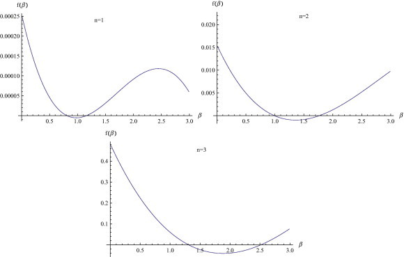
Determination of first excited mode with $\beta$ as an unknown parameter.

Table 4.

Bifurcation value of $\beta$.

Cases	Value of $\beta$ Considered	Bifurcation Value
		Without diffusion	With diffusion
1	$0.75$	$0.750435$	$0.810383$
2	$0.75$	$0.750367$	$0.810239$
3	$0.75$	$0.750387$	$0.809841$
4	$0.70$	$0.700381$	$0.756276$

Table 5.

Bifurcation values of ${\gamma }_1$ and${\gamma }_2$.

Cases	${\gamma }_1$	Without diffusion	With diffusion	${\gamma }_2$	Without diffusion	With diffusion
1	$0.125$	$0.124708$	$0.087493$	$0.2$	$0.199660$	$0.161489$
2	$0.125$	$0.124752$	$0.0873489$	$0.25$	$0.249586$	$0.196281$
3	$0.175$	$0.17471$	$0.133485$	$0.2$	$0.199694$	$0.161499$
4	$0.125$	$0.124726$	$0.0875375$	$0.2$	$0.199680$	$0.161530$

4. Numerical solutions

Four cases with the variation of $\beta$, the transmission coefficient, ${\gamma }_1$, the recovery coefficient in the infectious class and ${\gamma }_2$, the recovery coefficient in the diagnosed class have been chosen as given in Table 6 . Numerical solutions are obtained both with and without diffusion for all cases specified in Table 6.

Table 6.

Four cases.

Case	Transmission coefficient$(\beta )$	Recovery coefficient$({\gamma }_1)$	Recovery coefficient $({\gamma }_2)$
1	$0.75$	$0.125$	$0.2$
2	$0.75$	$0.125$	$0.25$
3	$0.75$	$0.175$	$0.2$
4	$0.7$	$0.125$	$0.2$

4.1. Solutions of SEIJR model without diffusion (case 1)

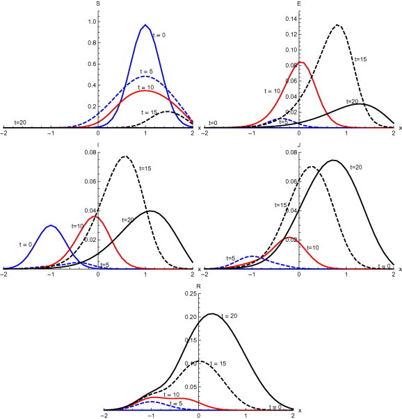
Fig. 3 , shows the output with initial condition $(i)$ and without diffusion. Here the susceptible population decreases slowly in the first five days of disease but after that there is a rapid decrease till $t=20$  days. There is a rapid increase in population exposed to disease in the first five days and this increase continues till $t=10$. It slows down however after five days. After ten days there is a quick decrease in exposed individuals. Only a few individuals are in the exposed compartment after fifteen days. There is a slow increase in infected individuals till the fifth day. But a sudden increase in infected is observed in the next five days. After reaching maximum level, a decline in infected is observed till $t=15$. With the increase of infected individuals, the number of diagnosed has also increased rapidly but after attaining the maximum in the first ten days of disease, there is a slow decrease till $t=15$. After that a quick decline is observed at $t=20$. Recovered individuals increase slowly in first ten days of disease but after that a rapid increase in recovery is observed.

Fig. 3.

Solutions with initial condition $(i)$ and without diffusion.

Fig. 4 , shows the output with initial condition $(\mathit{ii})$ without diffusion. Here the proportion of the susceptible population decreases rapidly between 5–10 days and after that there is very low level of susceptible population. The population becomes exposed very quickly during first five days. After ten days, there is a sudden decrease which continues till $t=20$  days. Infected individuals increase for the first ten days with rapid increase between 5–10 days. After that there is a rapid decrease till $t=15$. Then a decrease occurs slowly till $t=20$. The proportion of diagnosed shows an increase till $t=10$ and after that diagnosed individuals reduce with a quick fall between $t=15$ and 20 days. Recovery is slow initially but after t  = 10, it is fairly quick.

Fig. 4.

Solutions with initial condition $(\mathit{ii})$ and without diffusion.

Fig. 5 , shows the output with initial condition $(\mathit{iii})$ and without diffusion. The behavior of the susceptible is quite different as compared to the initial conditions $(i)$ and $(\mathit{ii})$. Susceptible move to the right of the initial domain of concentration slowly and slowly without much change in proportion of susceptible population. Initially the main concentration of the susceptible population is in the interval $[0\text{,}2]$ but at $t=20$ this shifts to $[0.6\text{,}2]$. More and more of the population become exposed during t  = 10 to 20 days of onset of the disease. During the first five days of the onset of SARS, the proportion of infected people goes down in its domain $[-2\text{,}0]$ and after that starts moving to domain $[0\text{,}2]$ with gradual increase. A sharp increase is observed between $t=10$ and 20 days $[0\text{,}1]$. The number of diagnosed individuals increases during the first five days in the domain $[-2\text{,}0]$. After that diagnosed individuals decrease with a slow pace. Also the concentration of the diagnosed moves to the domain $[0\text{,}2]$. A rapid increase of diagnosed can be seen between $t=15$ and 20 days. Till $t=10$ recovery increases in the domain $[-2\text{,}0]$ and slowly moves to domain $[0\text{,}1]$. From $t=15$ to $t=20$ recovery attains maximum values in the domain $[0\text{,}1]$.

Fig. 5.

Solutions with initial condition $(\mathit{iii})$ and without diffusion.

Fig. 6 , shows the output with the initial condition $(\mathit{iv})$ and without diffusion. Susceptible individuals decrease rapidly after $t=5$. At $t=15$, the susceptible reduce to a very low level of concentration. Exposed individuals reach the maximum level in first five days and after that start reducing. Infected individuals increase till $t=10$ and after that there is a sudden fall till $t=20$. Diagnosed individuals increase in the first ten days and after that there is a gradual decrease. There is gradual increase in recovered individuals as shown in Fig. 6.

Fig. 6.

Solutions with initial condition $(\mathit{iv})$ and without diffusion.

4.2. Solutions of SEIJR model with diffusion (case 1)

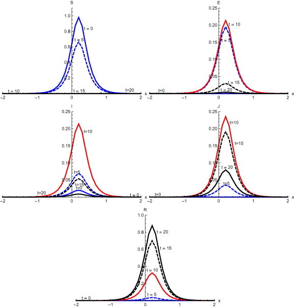
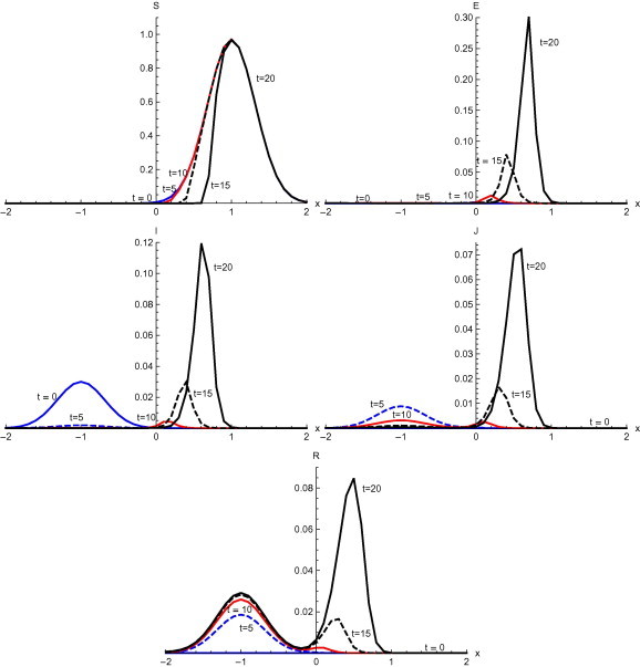
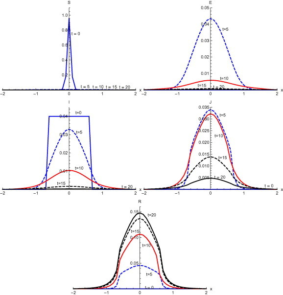
Fig. 7 , shows the output with initial condition $(i)$ and with diffusion. With the inclusion of diffusion in the system, susceptible spread in the entire region at $t=5$ with peak value $0.2228567$. Initially exposed are mainly confined in domain $[-1\text{,}1.5]$. At $t=5$ exposed spread in the domain $[-1\text{,}1.5]$ with peak value $0.118055$. At $t=10$, exposed spread in the whole domain with peak value $0.068133$. After this a rapid decrease in the exposed individuals occurs. Infected individuals spread in the whole domain $[-2\text{,}2]$ with the passage of time and at $t=10$, infected individual attains its maximum with peak value $0.077894$. After this there is a fall in the infected individuals and at $t=20$, there is very low level of infected individuals. A steady spread of diagnosed is observed in the main domain $[-2\text{,}2]$. At $t=10$ diagnosed are observed in the entire domain with peak value $0.105364$. After $t=10$, there starts a decrease in the diagnosed population. Recovery starts spreading in the domain and at $t=20$  days, it completely spreads over the whole domain with peak value $0.383669$.

Fig. 7.

Solutions with initial condition $(i)$ and with diffusion.

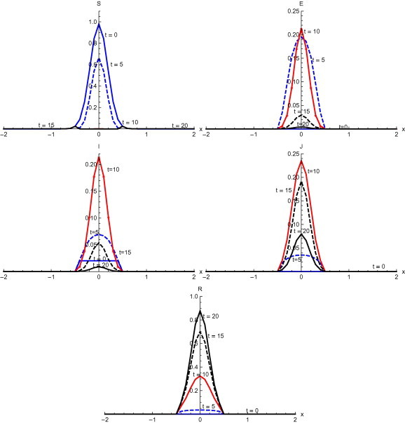
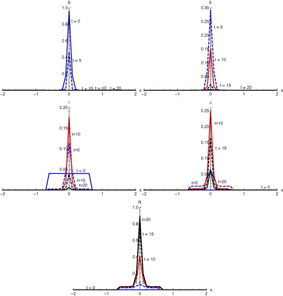
Fig. 8 , represents the results with the initial condition $(\mathit{ii})$ and with diffusion. Susceptible quickly spreads in the whole domain $[-2\text{,}2]$ with low peak value $0.129482$ at $t=5$. In the first five days exposed spread in the domain $[-1\text{,}1]$ with peak value $0.117691$. In first ten days, exposed spread to whole domain with peak value $0.040644$. After ten days the maximum proportion of population gets infected and spread in the main domain $[-2\text{,}2]$. Though the population in the whole domain $[-2\text{,}2]$ is infected but main concentration of infected lies in domain $[-1\text{,}1]$. At time $t=10$, diagnosed spread over the whole domain with peak value $0.085846$. Diagnosed thereafter start reducing and at time $t=15$  days reduce to peak value $0.051532$. Recovery starts slowly and spread to domain $[-0.6\text{,}0.6]$ at $t=5$. At $t=20$, recovered are spread over the whole domain with peak value $0.311524$.

Fig. 8.

Solutions with initial condition $(\mathit{ii})$ and with diffusion.

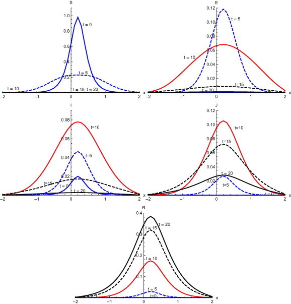
Fig. 9 , shows the results with the initial condition $(\mathit{iii})$ and with diffusion. Susceptible spread from the initial domain of concentration $[0\text{,}2]$ to the domain $[-1.5\text{,}2]$ at $t=5$. After 5 days, susceptible start moving back. Susceptible are confined to the domain $[0.5\text{,}2]$ at $t=15$. Exposed individuals also shifts from domain $[-2\text{,}0]$ to $[0\text{,}2]$ with the passage of time. Initially infectives are confined to domain $[-2\text{,}0]$. Infected spread at very slow pace and a small pulse with peak value $0.004476$ can be observed at $t=5$. After 10 days, the domain of concentration of infected people moves to $[-1\text{,}1]$. At $t=15$, infection spread in the whole domain $[-2\text{,}2]$. At $t=5$, a small proportion of diagnosed remain in the domain $[-2\text{,}0]$. There is, however, a rapid increase in the number of diagnosed with peak value $0.074575$ at $t=20$. At $t=5$, recovery is restricted to the domain $[-2\text{,}0]$. After 20 days, recovered spread in the domain $[-2\text{,}2]$, with peak value $0.206879$.

Fig. 9.

Solutions with initial condition $(\mathit{iii})$ and with diffusion.

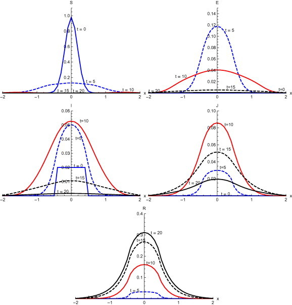
Fig. 10 , shows the results with initial condition $(\mathit{iv})$ and with diffusion. A sudden fall in the susceptible is observed at $t=5$ with peak value $0.005466$. During the same time, exposed spread to domain $[-1.5\text{,}1.5]$ with peak value $0.043322$. At $t=10$, infected spread in the domain $[-1.8\text{,}1.8]$ with peak value $0.010391$. At $t=5$, diagnosed spread to domain$[-1\text{,}1]$ with peak value $0.033966$. Diagnosed spread further in the domain $[-1.8\text{,}1.8]$ at $t=15$ with peak value $0.01385$. Recovery initially occurs in the domain $[-1\text{,}1]$ at $t=5$ with peak value $0.045636$. There is a further increase of recovered at $t=10$ with peak value $0.106593$. At $t=20$ there is maximum recovery with peak value $0.147773$.

Fig. 10.

Solutions with initial condition $(\mathit{iv})$ and with diffusion.

4.3. Other cases

Graphs of numerical solutions of Cases 2–4, obtained both with and without diffusion, for all cases specified in Table 6 are quite similar to Case 1. Thus graphs for Cases 2–4 are not reproduced here. Summarized results for Cases 2–4 are shown in Table 7, Table 8, Table 9, Table 10 . Here $S_j\text{,}{E}_j\text{,}{I}_j$ and $R_j$ for $j=(i)\text{,}(\mathit{ii})\text{,}(\mathit{iii})$ and $(\mathit{iv})$ represent the proportion of susceptible, exposed, infected and recovered population at critical points in the domain $[-2\text{,}2]$ without and with diffusion, for the initial condition $(i)\text{,}(\mathit{ii})\text{,}(\mathit{iii})$ and $(\mathit{iv})$ respectively. The following description is based on the information provided in Table 7, Table 10.

Table 7.

Peak values of susceptible (S) and exposed (E) (without diffusion).

Case	t	$S_{(i)}$	$S_{(\mathit{ii})}$	$S_{(\mathit{iii})}$	$S_{(\mathit{iv})}$	$E_{(i)}$	$E_{(\mathit{ii})}$	$E_{(\mathit{iii})}$	$E_{(\mathit{iv})}$
1	00	98.0	98.0	97.0	96.0	0.00	0.00	0.00	0.00
	05	66.4	66.4	96.9	46.3	19.5	19.5	0.171	29.0
	10	0.073	2.34	96.8	0.039	21.3	21.3	1.25	0.039
	15	0.001	2.36	96.7	0.059	2.94	2.94	7.87	2.05
	20	0.002	2.38	96.6	0.078	0.410	0.410	30.1	0.288
2	00	98.0	98.0	97.0	96.0	0.00	0.00	0.00	0.00
	05	68.2	68.2	96.9	48.6	18.3	18.3	0.161	27.57
	10	0.156	2.34	96.9	0.039	22.6	22.6	1.12	15.7
	15	0.001	2.36	96.8	0.059	3.12	3.12	7.38	2.16
	20	0.003	2.38	96.7	0.078	0.434	0.434	26.3	0.303
3	00	98.0	98.0	97.0	96.0	0.00	0.00	0.00	0.00
	05	68.7	68.7	96.9	49.3	18.0	18.0	0.159	27.3
	10	0.151	2.34	96.8	0.039	22.8	22.8	1.11	15.9
	15	0.001	2.36	96.8	0.059	3.15	3.15	7.36	2.18
	20	0.002	2.38	96.7	0.078	0.438	0.438	26.2	0.306
4	00	98.0	98.0	97.0	96.0	0.00	0.00	0.00	0.00
	05	69.7	68.2	96.9	50.5	17.4	18.3	0.155	26.6
	10	0.181	2.34	96.8	0.039	23.4	22.6	1.04	16.3
	15	0.001	2.36	96.8	0.059	3.24	3.12	6.92	2.23
	20	0.002	2.38	96.7	0.078	0.451	0.434	22.7	0.313

Table 8.

Peak values of infective (I) and recovered (R) (without diffusion).

Case	t	$I_{(i)}$	$I_{(\mathit{ii})}$	$I_{(\mathit{iii})}$	$I_{(\mathit{iv})}$	$R_{(i)}$	$R_{(\mathit{ii})}$	$R_{(\mathit{iii})}$	$R_{(\mathit{iv})}$
1	002.00	2.00	3.00	4.00	0.00	0.00	0.00	0.00	–
	05	6.91	6.91	0.189	11.4	3.53	3.53	1.86	6.61
	10	21.4	21.4	0.416	17.7	32.4	32.4	2.59	41.1
	15	5.37	5.37	2.98	3.91	69.9	69.9	2.833	74.8
	20	0.891	0.891	11.9	0.632	87.6	87.6	8.47	89.4
2	00	2.00	2.00	3.00	4.00	0.00	0.00	0.00	0.00
	05	6.55	6.55	0.189	10.9	3.71	3.71	2.01	6.98
	10	21.7	21.7	0.403	18.1	33.7	33.7	2.71	43.2
	15	5.64	5.64	2.62	4.09	73.4	73.4	2.89	78.3
	20	0.942	0.942	11.6	0.665	90.3	90.3	8.39	91.9
3	00	2.00	2.00	3.00	4.00	0.00	0.00	0.00	0.00
	05	6.08	6.08	0.141	10.1	3.92	3.92	2.01	7.35
	10	19.8	19.8	0.377	16.2	34.8	34.8	2.66	43.9
	15	4.72	4.72	2.48	3.38	72.5	72.5	2.86	77.0
	20	0.742	0.742	10.9	0.521	88.9	88.9	8.82	90.5
4	00	2.00	2.00	3.00	4.00	0.00	0.00	0.00	0.00
	05	6.20	6.55	0.189	10.4	3.32	3.71	1.86	6.27
	10	21.9	21.7	0.394	18.4	30.5	33.7	2.60	39.4
	15	5.82	5.64	2.35	4.23	68.7	73.4	2.83	73.8
	20	0.975	0.942	11.2	0.687	87.1	90.3	7.26	89.0

Table 9.

Peak values of susceptible (S) and exposed (E) (with diffusion).

Case	t	$S_{(i)}$	$S_{(\mathit{ii})}$	$S_{(\mathit{iii})}$	$S_{(\mathit{iv})}$	$E_{(i)}$	$E_{(\mathit{ii})}$	$E_{(\mathit{iii})}$	$E_{(\mathit{iv})}$
1	00	98.0	98.0	97.0	96.0	0.00	0.00	0.00	0.00
	05	22.9	12.9	48.4	0.547	11.8	11.8	1.18	4.33
	10	0.595	0.859	34.9	0.021	6.81	4.06	8.39	0.584
	15	0.001	0.002	15.1	0.002	0.886	0.531	13.2	0.077
	20	0.002	0.003	0.004	0.005	0.123	0.077	3.05	0.017
2	00	98.0	98.0	97.0	96.0	0.00	0.00	0.00	0.00
	05	23.8	13.7	48.5	0.669	0.111	11.2	1.09	4.30
	10	0.728	0.917	34.9	0.024	0.072	4.25	7.99	0.603
	15	0.002	0.002	15.7	0.003	0.009	0.556	13.1	0.079
	20	0.003	0.004	0.005	0.007	0.001	0.079	3.24	0.016
3	00	98.0	98.0	97.0	96.0	0.00	0.00	0.00	0.00
	05	23.9	13.9	48.5	0.683	11.0	11.1	1.10	4.33
	10	0.760	0.949	35.0	0.026	7.21	4.29	7.97	0.609
	15	0.001	0.002	15.9	0.003	0.942	0.561	13.2	0.079
	20	0.003	0.003	0.005	0.005	0.130	0.081	3.28	0.017
4	00	98.0	98.0	97.0	96.0	0.00	0.00	0.00	0.00
	05	24.4	13.7	48.5	0.700	10.7	11.2	1.10	4.35
	10	0.876	0.917	7.78	0.029	7.39	4.25	7.78	0.615
	15	0.001	0.002	16.7	0.003	0.966	0.556	13.0	0.080
	20	0.002	0.004	0.005	0.005	0.134	0.079	3.51	0.017

Table 10.

Peak values of infective (I) and recovered (R) (with diffusion).

Case	t	$I_{(i)}$	$I_{(\mathit{ii})}$	$I_{(\mathit{iii})}$	$I_{(\mathit{iv})}$	$R_{(i)}$	$R_{(\mathit{ii})}$	$R_{(\mathit{iii})}$	$R_{(\mathit{iv})}$
1	00	2.00	2.00	3.00	4.00	0.00	0.00	0.00	0.00
	05	4.63	5.03	0.448	3.30	2.94	3.21	1.84	4.56
	10	7.79	5.27	3.61	1.04	17.4	16.0	2.78	10.7
	15	1.72	1.07	7.73	0.166	32.0	26.7	10.5	13.7
	20	0.272	0.167	3.98	0.028	38.4	31.2	20.7	14.8
2	00	2.00	2.00	3.00	4.00	0.00	0.00	0.00	0.00
	05	3.10	3.40	1.99	4.89	3.10	3.40	1.99	4.89
	10	18.1	16.8	2.91	11.2	18.1	16.8	2.91	11.2
	15	33.3	27.8	10.9	14.1	33.3	27.8	10.9	14.1
	20	39.2	31.7	21.6	14.9	39.2	31.7	21.6	14.9
3	00	2.00	2.00	3.00	4.00	0.00	0.00	0.00	0.00
	05	4.08	4.46	0.394	2.95	3.25	3.57	1.99	5.03
	10	7.11	4.77	3.20	0.895	18.4	16.9	2.89	11.1
	15	1.48	0.905	7.05	0.135	32.8	27.3	11.1	13.9
	20	0.223	0.135	3.65	0.022	38.6	31.3	21.3	14.8
4	00	2.00	2.00	3.00	4.00	0.00	0.00	0.00	0.00
	05	4.21	4.82	0.422	3.21	2.79	3.39	35.1	4.45
	10	7.99	5.36	3.32	1.07	16.5	16.8	2.78	10.5
	15	1.84	1.11	7.53	0.174	31.3	27.8	9.98	13.5
	20	0.294	0.174	4.27	0.029	37.8	31.7	19.9	14.6

In Case 2, there is an increase in the recovery coefficient of diagnosed individual, ${\gamma }_2=0.25$ while keeping values of transmission coefficient, $\beta$ and recovery rate of infected, ${\gamma }_1$ the same as in Case 1. There is a slow decrease in susceptible population as compared to Case 1, for all initial conditions, with and without diffusion in the system. Fewer individuals seem to be exposed and infected to disease in the first five days with conditions $(i)\text{,}(\mathit{ii})$ and $(\mathit{iv})$ and after five days their proportion is greater in comparison to Case 1. But with condition $(\mathit{iii})$, there is a smaller proportion of exposed all the time. There is higher proportion of recovered in Case 2 as compared to Case 1, both with and without diffusion.

In Case 3, there is increase in recovery rate of infected individuals, ${\gamma }_1=0.175$ as compared to Case 1 and Case 2. There is slow decrease in susceptible population during the first five days for condition $(i)$–$(\mathit{iv})$, with and without diffusion as compared to Cases 1 and 2. Initially exposed are small in proportion as compared to Case 1 but after five days the proportion of exposed is more than in Case 1 with initial condition $(i)\text{,}(\mathit{ii})$ and $(\mathit{iv})$. On the other hand with initial condition $(\mathit{iii})$, there is a decrease in exposed individuals. Population of infectious reduces remarkably in Case 3. Diagnosed class also has a decrease in individuals. More individuals recover in Case 3 as compared to Case 1. But the recovered population in Case 3 is less than that in Case 2.

In Case 4, there is a reduced value of the transmission coefficient, $\beta =0.7$ as compared to Cases $1\text{,}2\text{,}3$. This causes a slow decrease in the susceptible population as compared to Cases $1\text{,}2$ and 3 till $t=10$. Exposed behave similarly as in Cases 2 and 3 with the number of individuals first decreasing and then increasing as compared to Case 1. Population of infected is less than Cases 1 at t  = 5. After that, till t  = 20 days, more infected individuals are observed in Case 4 as compared to Cases 1. Recovered individuals slow down here and the number of recovered population is less in this case as compared to other cases.

5. Discussion and conclusion

An SEIJR Model for SARS (Chowell et al. [5]) is considered with the inclusion of diffusion in the system. Four different initial conditions are taken for the population distribution. The equation governing the system are solved numerically using operator splitting method. The reproduction number ${\mathfrak{R}}_0$ is calculated for the disease. It is shown that disease dies out for ${\mathfrak{R}}_0<1$, in disease free equilibrium. It however prevails for endemic equilibrium, where ${\mathfrak{R}}_0>1$ as shown in Table 11 . Stability of solutions with and without diffusion is established using Routh–Hurwitz conditions as shown in Tables Table 2, Table 3 The value of the reproduction number ${\mathfrak{R}}_0$ depends on ten parameters. The parameters transmission coefficient $\beta$, recovery rate in infectious class ${\gamma }_1$ and recovery coefficient in diagnosed ${\gamma }_2$ have been varied to observe the effects on the spread of disease. Hence four cases are produced to see the effect on the spread of disease. Bifurcation values of transmission coefficient $\beta$ and recovery coefficients ${\gamma }_1$ and ${\gamma }_2$ are calculated. It is observed that diffusion causes an increase in the bifurcation value of $\beta$ and a decrease in the value of recovery coefficients. This shows that the system can be stable for larger value of $\beta$ and smaller values of recovery rates ${\gamma }_1$ and ${\gamma }_2$ in the presence of diffusion.

Table 11.

Peak values of infective at $t=20$.

Cases	Peak values for initial conditions				Reproductive number
	$(i)$	$(\mathit{ii})$	$(\mathit{iii})$	$(\mathit{iv})$
1	$0.891$	$0.891$	$11.90$	$0.632$	$2.83$
2	$0.942$	$0.942$	$11.60$	$0.665$	$2.64$
3	$0.742$	$0.742$	$10.90$	$0.521$	$2.58$
4	$0.975$	$0.942$	$11.20$	$0.687$	$2.64$

Table 2.

Routh–Hurwitz criterion of equilibrium without diffusion.

Case	Equilibrium point	$c_1$	$c_2$	$c_3$	$c_4$	$c_5$	Stable/Unstable
1	$P1$	$0.97677$	$6.902\times {10}^{-7}$	$0.20805$	$5.343\times {10}^{-6}$	$7.613\times {10}^{-12}$	Stable
2	$P2$	$1.02482$	$7.641\times {10}^{-11}$	$0.24969$	$6.903\times {10}^{-6}$	$1.114\times {10}^{-11}$	Stable
3	$P3$	$1.02416$	$6.560\times {10}^{-11}$	$0.23359$	$6.059\times {10}^{-6}$	$8.399\times {10}^{-12}$	Stable
4	$P4$	$0.97676$	$6.199\times {10}^{-11}$	$0.20804$	$5.109\times {10}^{-6}$	$6.421\times {10}^{-12}$	Stable

Where $c_1=p_1\text{,}{c}_2=p_5\text{,}{c}_3=p_1{p}_2-p_3$, $c_4=p_1{p}_2{p}_3+p_1{p}_5-(p_3^2+p_1^2{p}_4)$,

and $c_5=(p_1{p}_4-p_5)(p_1{p}_2{p}_3-p_3^2-p_1^2{p}_4)+p_1^2{p}_4{p}_5-(p_5{(p_1{p}_2-p_3)}^2+p_1{p}_5^2)$.

Table 3.

Routh–Hurwitz criterion of equilibrium with diffusion.

Case	Equilibrium point	$c_1$	$c_2$	$c_3$	$c_4$	$c_5$	Stable/ Unstable
1	$P1$	$1.0656$	$4.859\times {10}^{-8}$	$0.29522$	$0.00478$	$8.061\times {10}^{-7}$	Stable
2	$P2$	$1.11365$	$5.820\times {10}^{-8}$	$0.345648$	$0.006458$	$1.411\times {10}^{-6}$	Stable
3	$P3$	$1.1109$	$4.696\times {10}^{-8}$	$0.322143$	$0.004815$	$9.623\times {10}^{-8}$	Stable
4	$P4$	$1.06559$	$4.70\times {10}^{-8}$	$0.29521$	$0.004779$	$8.049\times {10}^{-7}$	Stable

Where $c_1=q_1\text{,}{c}_2=q_5\text{,}{c}_3=q_1{q}_2-p_3$, $c_4=q_1{q}_2{q}_3+q_1{q}_5-(q_3^2+q_1^2{q}_4)$ and $c_5=(q_1{q}_4-q_5)(q_1{q}_2{q}_3-q_3^2-q_1^2{q}_4)+q_1^2{q}_4{q}_5-q_5{(q_1{q}_2-q_3)}^2{q}_1{q}_5^2$.

Numerical solution with initial condition $(i)$, as shown in Fig. 3, Fig. 7, that in the absence of diffusion, only the population in the domain $[-1\text{,}1.5]$ becomes susceptible, but when diffusion is introduced susceptible spread over the whole domain in first five days. Similarly the exposed remain confined in the interval $[-1\text{,}1.5]$ in the absence of diffusion. But with diffusion population outside the domain $[-1\text{,}1.5]$ also become exposed to infection and after ten days exposed population spread to whole domain. With and without diffusion in the system, infection reached to its peak in first ten days. With the inclusion of diffusion, however, infection spreads over the whole domain $[-2\text{,}2]$. Recovered also follows the same pattern. Numerical solution of initial condition $(\mathit{ii})$, as shown in Fig. 4, Fig. 8, follows the same pattern as in condition $(i)$ with only difference in concentration of population in different domain. In the absence of diffusion infective population fluctuate inside the domain $[-.5\text{,}.5]$, but with diffusion in the system fluctuations follows with the spread in the whole domain after ten days Numerical solution with initial condition $(\mathit{iii})$, as shown in Fig. 5, Fig. 9, shows the main concentration of susceptible shifts slightly to right of domain $[0\text{,}2]$ in 20 days. Infected move to domain $[0\text{,}2]$ from domain $[-2\text{,}0]$ and with that diagnosed and recovered also follow the same pattern. With diffusion in the system Susceptible start spreading to the left of the domain $[-2\text{,}2]$ but are mainly confined in $[-0.8\text{,}2]$. Exposed grows in the smaller domain $[-1\text{,}0.5]$ first and then with passage of time spread in the domain $[-1.5\text{,}2]$. Infected shifts their domain from $[-2\text{,}0]$ to $[-1\text{,}2]$ followed with decrease, increase and then again decrease in proportion. Thus with diffusion more individuals get infected within a short time and infection spreads quickly and reaches its maximum in 15 days covering almost the whole domain. In the absence of diffusion the maximum number of infected are observed after twenty days in domain $[0\text{,}1]$, reflecting the intensity of infection more than that with diffusion during the same time. A large proportion of population is recovered with diffusion in the system during the same time as compared to without diffusion. Numerical solution with initial condition $(\mathit{iv})$, as shown in Fig. 6, Fig. 10, demonstrate that diffusion causes the infection to spread out from domain $[-.7\text{,}.7]$ to $[-2\text{,}2]$. The intensity of the infection also becomes less than the initial intensity as it spreads to $[-1.5\text{,}1.5]$.

It has been observed in Table 7, Table 10 that when recovery is improved in diagnosed class with an increased value of ${\gamma }_2$ as in Case 2, less proportion of population becomes infected and proportion of the recovered increases. Even better result is obtained with the greater recovery of infected with an increased value of ${\gamma }_1$ as shown in Case 3, where the proportion of recovered is higher than previous Case 2 even with a lower value of diagnosed recovery, ${\gamma }_2$. With recovery coefficients ${\gamma }_1$ the same and decreasing the transmission coefficient $\beta$ as in Case 4, recovery is observed to be slower than the original Case 1.

Conclusions are summarized as follows:

• •Initial population distribution plays a crucial role in the spread of disease.
• •Diffusion plays an important role in reducing the intensity of disease.
• •An increase in recovery of infective through intervention plays an effective role during the initial days of the onset of disease.
• •An increase in recovery of diagnosed plays a more effective role during the last days of disease.
• •Thus interventions are good tools to reduce the intensity of the disease.

References

- 1.Anderson R., May R. Oxford University Press; Oxford UK: 1991. Infectious Diseases of Humans: Dynamics and Control. [Google Scholar]
- 2.Chakraborty A., Singh M., Lucy D., Ridland P. Predator–prey model with prey-taxis and diffusion. Math. Comput. Model. 2007;46:482–498. [Google Scholar]
- 3.Chakraborty A., Singh M., Ridland M. Effect of prey-taxis on biological control of the two-spotted spider mite–a numerical approach. Math. Comput. Model. 2009;50:598–610. [Google Scholar]
- 4.Chen W.J., Wu K.C., Wu K.L., Lin M.H., Li C.X. Approach to the mechanism of cluster transmission of SARS by mathematical model. Chin. Trop. Med. 2004;4:20–23. [Google Scholar]
- 5.Chowell G., Fenimore P.W., Castillo-Garsow M.A., Castillo-Chavez C. SARS outbreak in Ontario, Hong Kong and Singapore: the role of diagnosis and isolation as a control mechanism. J. Theor. Biol. 2003;224:1–8. doi: 10.1016/S0022-5193(03)00228-5. [DOI] [PMC free article] [PubMed] [Google Scholar]
- 6.Diekmann O., Heesterbeek J.A.P., Metz J.A.J. On the definition and the computation of the basic reproduction ratio R0 in models for infectious diseases in heterogeneous populations. J. Math. Biol. 1990;28:365–382. doi: 10.1007/BF00178324. [DOI] [PubMed] [Google Scholar]
- 7.Driessche Van den P., Watmough J. Reproduction numbers and sub-threshold endemic equilibria for compartmental models of disease transmission. Math. Biosci. 2002;180:29–48. doi: 10.1016/s0025-5564(02)00108-6. [DOI] [PubMed] [Google Scholar]
- 8.Dye C., Gay N. Modeling the SARS epidemic. Science. 2003;300:884–1885. doi: 10.1126/science.1086925. [DOI] [PubMed] [Google Scholar]
- 9.Hethcote H.W. The mathematics of infectious diseases. SIAM. 2000;42(2000):599–653. [Google Scholar]
- 10.Gumel Abba B. Modelling strategies for controlling SARS outbreaks. R. Soc. 2004;271:2223–2232. doi: 10.1098/rspb.2004.2800. [DOI] [PMC free article] [PubMed] [Google Scholar]
- 11.Sapoukhina N., Tyutyunov Y., Arditi A. The role of prey-taxis in biological control. Am. Nat. 2003;162:61–76. doi: 10.1086/375297. [DOI] [PubMed] [Google Scholar]
- 12.Samsuzzoha Md., Singh M., Lucy D. Numerical study of an influenza epidemic model with diffusion. Appl. Math. Comput. 2010;217(7):3461–3479. [Google Scholar]
- 13.Md. Samsuzzoha, M. Singh, D. Lucy, A Study on numerical solutions of epidemic models (Ph.D. thesis), Swinburne University of Technology, Australia, 2012.
- 14.Wu K.C., Wu K.L., Chen W.J., Lin M.H., Li C.X. Mathematical model and prediction of epidemic trend of SARS. Chin. Trop. Med. 2004;3:421–426. [Google Scholar]
- 15.<http://www.who.int/csr/sars/en>, 2003
- 16.SARS special topics, 2003. <http://www.scichina.com/ZTYJ/kzzt.htm>.
- 17.Xia J.L., Yao C., Zhang G.K. Analysis of piecewise compartmental modeling for epidemic of SARS in Guangdon. Chin. J. Health Stat. 2003;20:162–163. [Google Scholar]
- 18.Yanenko N.N. Springer-Verlag; New York: 1971. The Method of Fractional Steps. [Google Scholar]
- 19.Yang H., Li X.W., Shi H., Zhao K.G., Han L.J. Fly dots spreading model of SARS along transportation. J. Remote Sens. 2003;7:251–255. [Google Scholar]