RLadyBug—An R package for stochastic epidemic models

Abstract

RLadyBug is an S4 package for the simulation, visualization and estimation of stochastic epidemic models in R. Maximum likelihood and Bayesian inference can be performed to estimate the parameters in a susceptible-exposed-infectious-recovered (SEIR) model, which is a stochastic model for describing a single outbreak of an infectious disease. The package is thus one step towards statistical software supporting parameter estimation, calculation of confidence intervals and hypothesis testing for transmission models.

1. Introduction

Understanding the dynamics and spread of infectious diseases is a key component in the design and analysis of defensive strategies. As a consequence, a multitude of epidemiological data on infectious diseases in animal, plant and human communities has been collected to gain insights into the underlying biological and epidemiological processes. The SIR (susceptible-infectious-recovered) model and its variants (S-Exposed-IR, SIS, etc.) are the mathematical tools most commonly used in such analyses.

This paper describes a software program for the statistical analysis of a single outbreak in a small population. Special focus is on the spatial spread between subpopulations arranged on a lattice. In veterinary or plant epidemiology such data arise from so-called transmission experiments, where one or more individuals in a controlled environment are inoculated with the infectious disease pathogen. Subsequently, the course of the epidemic is monitored through visual inspection, clinical testing and other methods. The aim ranges in veterinary epidemiology from quantifying disease transmission (Laevens et al., 1999, Stärk et al., 2000) to determining the effect of a vaccine (Dewulf et al., 2001, Meyns et al., 2004).

Because outbreaks induced by transmission experiments are planned and occur in a controlled environment, the produced outbreak data are especially rich. However, the mathematical setup of course also applies to the analysis of ordinary outbreaks. Interesting is also the application to entirely different areas such as the analysis of computer virus in a network (Wierman and Marchette, 2004), spread of the severe acute respiratory syndrome (SARS) (Donelly and Ghani, 2004) or outbreaks in the wards of a hospital (Grundmann and Hellriegel, 2006).

RLadyBug  is a package implemented in R (R Development Core Team, 2006) providing functionality for the simulation, visualization and estimation in stochastic epidemic models. It enwraps the functionality of the Java program used in Höhle et al. (2005) by S4 classes and adds a volume of methods for the visualization of outbreak data and their estimation results. The aim of this paper is to describe the features of the package in order to make it accessible to statisticians and statistically trained epidemiologists who are looking for software to analyse their infectious disease data. Less attention is thus given to the statistical particulars, which are explained in Höhle et al. (2005).

This paper is organized as follows: Section 2 gives a short introduction to stochastic epidemic models, Section 3 introduces the package and illustrates its use by providing the corresponding R code for analyzing a transmission experiment with classical swine fever virus (CSFV). Section 4 provides a discussion.

2. Stochastic epidemic models

With focus on the software dimension, only a short introduction to stochastic epidemic models in terms of the SEIR model is given. For a more thorough description see Andersson and Britton (2000).

A closed population P is hosted in k units. Each individual in P can be in one of the states susceptible, exposed, infectious or recovered. A spatial dimension is introduced by assuming that the k units are arranged in a $k=k_1\times k_2$ lattice. At the beginning of the outbreak, $t=0$, the number of susceptibles in each unit is $\mathit{S}(0)=(n_1,\dots ,n_k)$, the number of exposed is $\mathit{E}(0)=(m_1,\dots ,m_k)$ and the number of infectious is $\mathit{I}(0)=(0,\dots ,0)$. At time t, an individual j in unit $u_j$ meets infectious at rate

$${\lambda }_{u_j}(t)=\beta I_{u_j}(t)+{\beta }_n\sum _{u\in N(u_j)}{I}_u(t)\text{,}$$ (1)

where $N(u_j)$ denotes the neighbors of $u_j$ (e.g. in the four compass directions). Furthermore, $\beta$ quantifies the within unit transmission rate, whilst ${\beta }_n$ quantifies the transmission rate between neighboring units. If a susceptible meets an infectious it becomes exposed. After being exposed at time $E_j$ an individual j has a gamma-distributed incubation time $T_E^j\sim \mathcal{G}a({\gamma }_E,{\delta }_E)$ before becoming infectious, i.e. starting from time $I_j=E_j+T_E^j$, j can infect others. Similarly, the infectious period lasts for $T_I^j\sim \mathcal{G}a({\gamma }_I,{\delta }_I)$ after which recovery occurs, hence $R_j=I_j+T_I^j$ labels the time of recovery.

Objective of analyzing outbreak data with SEIR models is the estimation of the parameters $\mathit{\theta }=(\beta ,{\beta }_n,{\gamma }_E,{\delta }_E,{\gamma }_I,{\delta }_I)$, which permit the effect of control measures to be studied and to generalize the results to different settings. RLadyBug  is a tool to accomplish this ambition.

3. The RLadyBug package

Where applicable, RLadyBug  uses the new S4 class system of R implemented in the methods package. This implies a more explicit class system requiring the programmer to define classes, slots and generics explicitly (Chambers, 1998). Fig. 1 shows the object oriented hierarchy of the package: The classes LBExperiment and LBLayout represent the data layer, LBOptions the algorithmic component and LBInference the results. With the help of the rJava package (Urbanek, 2006), this S4 framework is connected to the functionality of an underlying Java program performing the computationally intensive operations.

Fig. 1.

The object hierarchy of the RLadyBug S4 classes.

3.1. Simulation and visualization

To get an understanding of the SEIR model specified in Section 2, simulation based on the Sellke construction (Andersson and Britton, 2000) is utilized to generate data from the model. Code wise, this is accomplished by creating an object of class LBExperiment using the simulate function. Several visualizations of the experiment data can then be generated by plot, e.g. the type=state ${}^{\sim }$ time $|$ position argument shows $S_u(t),E_u(t)$ and $I_u(t)$ as a function of time for each unit u in the lattice. The below stated code creates a simulated epidemic in a $1\times 3$ lattice, see Fig. 2 . Initially $\mathit{S}(0)=(10,9,10)$ and $\mathit{E}(0)=(0,1,0)$.

>	$\text{library("RLadyBug")}$
>	$\text{layout <- new("LBLayout", S0 = matrix(c(10, 9, 10), 1, 3),}$
+			E0 = matrix(c(0, 1, 0), 1, 3))
>	$\text{options <- new("LBOptions", initBeta = list(init = 0.125),}$
+		initBetaN = list(init = 0.018), initIncu = list(g = 6.697, d = 0.84),
+		initInf = list(g = 1.772, d = 0.123))
>	plot(simulate(options, layout = layout), type = state${}^{\sim }$time$|$position)

Further views of LBExperiment objects can be generated using type=state ${}^{\sim }$ time or type=state ${}^{\sim }$ 1 $|$ position as arguments in plot. The former shows $S(t),E(t)$ and $I(t)$, with e.g. $S(t)={\sum }_{u=1}^k{S}_u(t)$, the latter creates an animation illustrating the course of the epidemic by plotting the state given position for a set of fixed time points. As exemplification, the code below uses a $8\times 16$ lattice with 15 individuals in each unit (a realistic setup for a pig farm) and creates a 20-picture animation of the epidemic. Fig. 3 shows the eighth picture of this sequence: Each stacked bar shows the current ($t=58.9$ days) percentage of susceptible, exposed, infectious and recovered in the unit.

$\text{>E0 <- matrix(0, 8, 16)}$

$\text{>E0[4, 8] <- 1}$

$\text{>S0 <- matrix(15, 8, 16) - E0}$

$\text{>exp <- simulate(options, layout = new("LBLayout", S0 = S0, E0 = E0))}$

$\text{>plot(exp, type = state}$${}^{\sim }$$\text{1}$$|$$\text{position, options = list(noOfPics = 20))}$

Fig. 2.

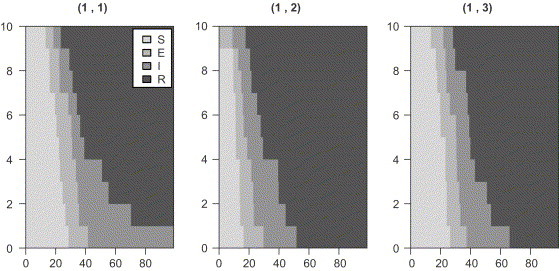
$S_u(t)$, $E_u(t)$, $I_u(t)$ and $R_u(t)$ for the three units in a $1\times 3$ lattice layout.

Fig. 3.

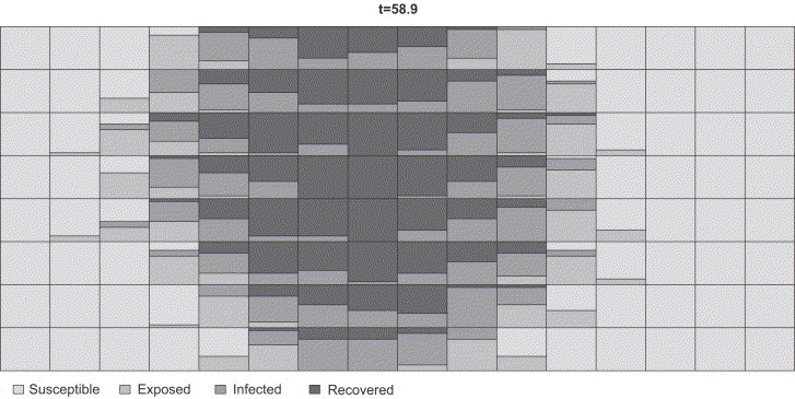
Snapshot of the animation illustrating the outbreak in a $8\times 16$ lattice.

3.2. Test data

Besides the ability to simulate data, the package contains several data sets from human and veterinary epidemiology. Amongst others are the Smallpox Epidemic in Abakaliki, Nigeria, analyzed e.g. in Andersson and Britton (2000) or O’Neill and Becker (2001), and the data from CSFV experiments by Laevens et al. (1999) and Dewulf et al. (2001). The next section describes a statistical analysis of the experiment by Laevens et al. (1999) using RLadyBug. In this experiment the spread of CSFV was investigated in a $1\times 3$ layout with $\mathit{S}(0)=(5,5,6)$ and $\mathit{E}=(0,1,0)$ slaughter pigs. Every second day all pigs still alive were investigated using a virus isolation test based on blood plasma.

3.3. Analysis of an CSFV transmission experiment

For full data, i.e. with known $E_j,I_j,R_j$ event times for all individuals, RLadyBug  provides likelihood or Bayesian inference for $\mathit{\theta }=(\beta ,{\beta }_n,{\gamma }_E,{\delta }_E,{\gamma }_I,{\delta }_I)$. Details about the underlying equations leading to the log-likelihood and posterior distribution can be found in Höhle et al. (2005).

In practice, however, $E_j$ is unobservable. A typical assumption is thus to assume a fixed and known incubation time c and hence compute $E_j$ as $E_j=I_j-c$. This was also done in the CSFV experiment by assuming $c=6$. With this assumption all event times are known and can be illustrated as in Fig. 4 :

$\text{>data("laevensML")}$

$\text{>plot(laevensML, type = individual}$${}^{\sim }$$\text{time}$$|$position)

The individual 12:01 was inoculated at time $t=0$. By maximization of the log-likelihood the maximum likelihood estimators are readily determined using RLadyBug. Nonetheless, assuming a fixed and known incubation time is not very realistic. Höhle et al. (2005) therefore use a Bayesian framework to handle the missing but gamma-distributed exposure times. Unknown (or censored) waiting times $T_E^j\sim \mathcal{G}a({\gamma }_E,{\delta }_E)$ are imputed and updated through a Gibbs-within-Metropolis–Hastings Markov Chain Monte Carlo (MCMC) algorithm.

Fig. 4.

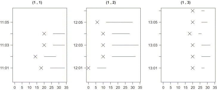
Infectious period of each individual ($x\mathrm{y}:\mathit{id}$) in the CSFV example. Crosses denote the time of exposure (in days), lines connect the $I_{\mathit{xy}:\mathit{id}}$ and $R_{\mathit{xy}:\mathit{id}}$ events.

A Bayesian-analysis of the CSFV data with unknown exposure times could be conducted by the following code:

$\text{>data("laevens")}$

$\text{>inf.mcmc <- seir(laevens, laevens.opts)}$

Instead of creating the necessary LBOptionsMCMC object by hand, the call to data also loads an appropriate object laevens.opts for MCMC estimation. For example:

$\text{>algo(laevens.opts)}$

samples	thin	burnin
2500	25	50000

shows the requested number of samples to draw from the posterior together with the burn-in and thinning rate; a total of samples*thin+burnin samples are generated. The results are as follows.

$\text{>inf.mcmc}$

An object of class LBInferenceMCMC

Parameter Estimations (posterior mean from 2500 samples):
Parameter:
beta	betaN	gammaE	deltaE	gammaI	deltaI
0.03706	0.02837	56.82000	9.37400	2.16200	0.25640
StandardErrors (posterior std.dev. from 2500 samples):
beta	betaN	gammaE	deltaE	gammaI	deltaI
0.018500	0.009481	45.510000	7.761000	0.738100	0.097760

The results of the MCMC inference are provided as realizations from the Markov chain having the posterior distribution of $\mathit{\theta }$ as stationary distribution. Access to the samples is obtained through the samplePaths method—this makes allowance for further processing using e.g. the coda (convergence diagnostic and output analysis) or boa (Bayesian output analysis) packages from the Comprehensive R Archive Network (Plummer et al., 2006, Smith, 2005). To exemplify, the sampling paths and the marginal posterior of $\beta$ are inspected in Fig. 5 by

$\text{>samples <- mcmc(samplePaths(inf.mcmc))}$

$\text{>plot(samples[, "beta"])}$

A matter of particular interest in the CSFV experiment is the relationship between $\beta$ and ${\beta }_n$—especially whether there is a difference in spread within the pen and between neighboring pens. The following code uses the plot method for LBInferenceMCMC objects to generate Fig. 6 and to display the posterior mean together with lower and upper boundaries of a 95%-highest posterior density (HPD) interval for $\beta /{\beta }_n$.

$\text{>betabetaN <- plot(inf.mcmc, which = "betabetaN")}$

$\text{>c(mean = betabetaN\$mean, betabetaN\$hpd)}$

mean	LB 95% HPD	UB 95% HPD
1.4740612	0.1245430	3.3158915

An important epidemiological quantity of an infectious disease is the basic reproduction ratio $R_0$, i.e. the expected number of new infections generated by a single infectious individual in a large susceptible population. In a multitype setup with k groups this can be computed as the largest eigenvalue of the $k\times k$ matrix containing the mean number of infectious contacts between all units (Andersson and Britton, 2000, Section 6.2). Samples from the posterior distribution of $R_0$ are generated by performing this computation for each posterior sample of $\mathit{\theta }$. The code stated below uses the method R0 to retrieve the samples for $R_0$ and thus to compute the posterior median together with a symmetric 95% credibility region.

$\text{>quantile(R0(inf.mcmc, laevens), c(0.025, 0.5, 0.975))}$

2.5%	50%	97.5%
0.3245193	0.6370434	1.2426485

Fig. 5.

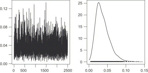
Sample path and kernel density of the $\beta$-samples generated using coda.

Fig. 6.

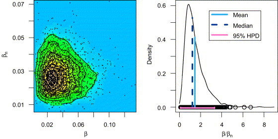
Left panel: 2D-Kernel estimated posterior density surface of $(\beta ,{\beta }_n)$. Right panel: 1D-Kernel estimate of the posterior density of $\beta /{\beta }_n$ together with posterior mean, posterior median and a 95%-HPD interval.

4. Discussion

In this paper we have illustrated the use of RLadyBug  for the simulation, visualization and estimation of infectious disease outbreak data. To our knowledge, the package is the first publicly available software for the estimation in stochastic epidemic models. By providing such specialist functionality within a standard software package as R we hope to make a thorough statistical analysis of infectious disease data a bit more routine.

Many extensions towards more complex and realistic models than provided by the package are imaginable. For example, the general multitype SEIR model (Andersson and Britton, 2000, Chapter 6) allows for more complicated neighbor dependencies: Letting $\mathit{\Lambda }(\mathit{\alpha })$ be a $k\times k$ matrix given as a function of the parameter vector $\mathit{\alpha }$, the transmission rates are given by $\mathit{\lambda }(t)=\mathit{\Lambda }(\mathit{\beta })\mathit{I}({\beta }_{\mathit{ij}}{)}^{\prime }$. Nearest neighborhood transmission as in (1) thus corresponds to ${\Lambda }_{\mathit{ij}}=\beta I(u_i=u_j)+{\beta }_{n}I(u_j\in N(u_j))$ and hence $\mathit{\alpha }=(\beta ,{\beta }_n)$. An alternative would be to let transmission from neighbors be a function of distance: ${\Lambda }_{\mathit{ij}}={\alpha }_1\exp (-{\alpha }_2\mathrm{dist}(u_i,u_j))$. Modifications of the Java code to handle the simulation and maximum likelihood estimation in such models should be feasible. However, obtaining MCMC estimates in case of missing data would require a substantial amount of work. The same comment applies if one wants to extend beyond the currently implemented waiting time distributions (gamma-distributed, exponential-distributed and constant).

The multitype model could also be applied to the handling of heterogeneous units exemplified by veterinary experiments quantifying the effect of a vaccine. Here, all individuals in specific units are vaccinated, thus having different parameters than individuals in non-vaccinated units. A Monte-Carlo approach could be employed to calculate sample sizes necessary to detect a certain difference in parameters with a given accuracy.

In addition, we are currently working on an implementation of the logistic-regression approach in Klinkenberg et al. (2002). This extension illustrates the benefits of providing a flexible and extensible package: the code is purely R-based exploiting the class structure of the package, while using the optimization routines of R for inference.

Sources, binaries and documentation of RLadyBug  are available for download from the Comprehensive R Archive Network http://cran.r-project.org/ under the GNU Public License. Once installed, the analyses of this article can be reproduced using $\text{demo("article-csda")}$.

References

- Andersson, H., Britton, T., 2000. Stochastic epidemic models and their statistical analysis. Springer Lectures Notes in Statistics, vol. 151, Springer, Berlin.
- Chambers, J.M., 1998. Programming with Data—A Guide to the S Language. Springer.
- Dewulf J., Laevens H., Koenen F., Vanderhallen H., Mintiens K. An experimental infection with classical swine fever in E2 sub-unit marker-vaccine vaccinated and in non-vaccinated pigs. Vaccine. 2001;19:475–482. doi: 10.1016/s0264-410x(00)00189-4. [DOI] [PubMed] [Google Scholar]
- Donelly C., Ghani A. Real-time epidemiology—understanding the spread of SARS. Significance. 2004;1:176–179. doi: 10.1111/j.1740-9713.2004.00066.x. [DOI] [PMC free article] [PubMed] [Google Scholar]
- Grundmann H., Hellriegel B. Mathematical modelling: a tool for hospital infection control. Lancet Infect. Dis. 2006;6:39–45. doi: 10.1016/S1473-3099(05)70325-X. [DOI] [PubMed] [Google Scholar]
- Höhle M., Jørgensen E., O’Neill P. Inference in disease transmission experiments by using stochastic epidemic models. J. Roy. Statist. Soc. Ser. C. 2005;54(2):349–366. [Google Scholar]
- Klinkenberg D., de Bree J., Laevens H., de Jong M. Within- and between-pen transmission of classical swine fever virus: a new method to estimate the basic reproduction ratio from transmission experiments. Epidemiol. Infect. 2002;128(2):293–299. doi: 10.1017/s0950268801006537. [DOI] [PMC free article] [PubMed] [Google Scholar]
- Laevens H., Koenen F., Deluyker H., de Kruif A. Experimental infection of slaughter pigs with classical swine fever virus: transmission of the virus, course of the disease and antibody response. Vet. Rec. 1999;145:243–248. doi: 10.1136/vr.145.9.243. [DOI] [PubMed] [Google Scholar]
- Meyns T., Maes D., Dewulf J., Vicca J., Haesebrouck F., de Kruif A. Quantification of the spread of Mycoplasma hyopneumonia in nursery pigs using transmission experiments. Prev. Vet. Med. 2004;66:265–275. doi: 10.1016/j.prevetmed.2004.10.001. [DOI] [PubMed] [Google Scholar]
- O’Neill P.D., Becker N.G. Inference for an epidemic when susceptibility varies. Biostatistics. 2001;2(1):99–108. doi: 10.1093/biostatistics/2.1.99. [DOI] [PubMed] [Google Scholar]
- Plummer, M., Best, N., Cowles, K., Vines, K., 2006. coda: output analysis and diagnostics for MCMC. R Package Version 0.10-5.
- R Development Core Team, 2006. R: A Language and Environment for Statistical Computing. R Foundation for Statistical Computing, Vienna, Austria, ISBN 3-900051-07-0.
- Smith, B.J., 2005. boa: Bayesian Output Analysis Program (BOA) for MCMC. R Package Version 1.1.5-2.
- Stärk K., Pfeiffer D., Morris R. Within-farm spread of classical swine fever virus—a blueprint for a stochastic simulation model. Vet. Quarterly. 2000;22(1):36–43. doi: 10.1080/01652176.2000.9695021. [DOI] [PubMed] [Google Scholar]
- Urbanek, S., 2006. rJava: Low-level R to Java interface. R Package Version 0.4-3.
- Wierman J., Marchette D. Modeling computer virus prevalence with susceptible-infected-susceptible model with reintroduction. Comput. Statist. Data Anal. 2004;45:3–23. [Google Scholar]