Deep DoseNet: A Deep Neural Network for Accurate Dosimetric Transformation between Different Spatial Resolutions and/or Different Dose Calculation Algorithms for Precision Radiation Therapy

Abstract

Purpose:

The purpose of this work is to introduce a novel deep learning strategy to obtain highly accurate dose plan by transforming from a dose distribution calculated using a low-cost algorithm (or algorithmic settings).

Methods:

25,168 slices of dose distribution are calculated using Eclipse treatment planning system V15.6 (Varian Medical Systems, Palo Alto, CA) on 10 patient CTs whose treatment sites ranging from lung, brain, abdomen and pelvis, with a grid size of 1.25×1.25×1.25mm using both anisotropic analytical algorithm (AAA) in 5mm resolution and Acuros XB algorithm (AXB) in 1.25mm resolution. The AAA dose slices, and the corresponding down sampled CT slices are combined to form a tensor with a size of 2×64×64, working as the input to the deep learning-based dose calculation network (Deep DoseNet), which outputs the calculated Acuros dose with a size of 256×256. The Deep DoseNet (DDN) consists of a feature extraction component and an upscaling part. The DDN converges after ~100 epochs with a learning rate of 10∧−4, using ADAM.

Results:

We compared up sampled AAA dose and DDN output with that of AXB. For the evaluation set, the average mean-square-error decreased from 4.7×10∧−4 between AAA and AXB to 7.0×10∧−5 between DDN and AXB, with an average improvement of ~ 12 times. The average Gamma index passing rate at 3mm3% improved from 76% between AAA and AXB to 91% between DDN and AXB. The average calculation time is less than 1 milliseconds for a single slice on a NVIDIA DGX workstation.

Conclusion:

DDN, trained with a large amount of dosimetric data, can be employed as a general-purpose dose calculation acceleration engine across various dose calculation algorithms.

1. Introduction

The success of modern radiotherapy modality, such as stereotactic body radiation therapy (SBRT)[1], stereotactic radiosurgery (SRS)[2], and adaptive therapy[3], critically depends on the accuracy and efficiency of dose calculation [4]. Coupled with the increasing utilization of the time intensive dose optimization techniques such as multi criteria optimization (MCO)[5], motion-considered or robust optimization[6] and trajectory optimization[7], the demand for high performance dose calculation increases continuously. In the past few decades, extensive research has been devoted to speed up Monte Carlo calculation [8], [9] by simplifying and approximating electron transport. Others[10] have taken a different route by solving the Linear Boltzmann Transport Equations (LBTE) deterministically, which describes statistically the behaviors of radiation particles during transport through medium without considering self-interaction, providing comparable accuracies to Mote Carlo method with improved calculation speed.

Deep learning[11], which extracts unique features and learns representations of data by multiple levels of abstraction through multiple processing layers such as convolutional layers, has sparked global interests in recent years and made major impact on several computational tasks[12] such as image reconstruction, classifications and recognition[13], disease detection[14], segmentation[15], super-resolution imaging[16], [17], image style transfer[18] and Dose prediction[19], [20]. Inspired by the success of super-resolution imaging, here we propose a deep learning strategy, named as Deep DoseNet (DDN), for dose calculation and optimization applications[21]. The technique is capable of not only up sampling the dose to speed up the calculation, but also transforming the dose calculated in one algorithm to another to enhance the accuracy of dose calculation.

2. Methods:

2.1. Single dose map super resolution:

Image super resolution is widely used to enhance the quality of a low resolution image, and its performance has improved substantially since the original work by Dong et al [16], which uses a three-layer deep convolutional neural network (SRCNN) to directly learn an end to end mapping between the low and high resolution images. Kim et al [22] increased the layer numbers of the CNN to 20 and used several training techniques including gradient clipping and skip connection to further boost the accuracy. Ledig et al [23] proposed to use Resblock [24] and GAN [25] to recover photo realistic textures from heavily down sampled images. Below we briefly summarize SRCNN (Fig. 1) [16], which is known for its simple and effective structure and forms the basis for more advanced networks and our DDN.

Fig. 1:

SRCNN structure

Given a low-resolution image X, SRCNN shown in Fig. 1 first upscales the image with cubic interpolation and uses it as the input G(X). SRCNN has three parts: feature extraction, nonlinear mapping and reconstruction. Feature extraction uses 9×9 convolution to generate 64 feature maps from the low-resolution image. The second part maps those 64 feature maps nonlinearly to 32 high-resolution patch representations with 1×1 convolution. The last part combines the 32 patch representations with 5×5 convolution to produce the final high-resolution image F(X). The mean square error (MSE) is employed as the loss function where i represents pixel i:

$$\mathit{\text{Loss}}={\sum }_{i=1}^n\Vert F\left(x_i\right)-G\left(x_i\right){\Vert }^2$$

and trained the network with 24,800 sub-images which are decomposed from 91 images, achieving the state-of-the-art results when compared with conventional methods[16].

2.2. Analytical Anisotropic Algorithm (AAA) vs Acuros XB (AXB)

Eclipse treatment planning system V15.6 (Varian Medical Systems, Palo Alto, CA) is used for the dose calculations. The system provides two main dose calculation algorithms: (i) the Analytical Anisotropic Algorithm (AAA) is an analytical calculation algorithm based on the pencil beam convolution superposition technique; and (ii) the grid based the Acuros XB (AXB), which solves the LBTE deterministically. AXB agrees the Monte Carlo method within 2% in low density lung, while the AAA shows a difference of 12%[10]. In bone and bone-tissue interface regions, dosimetric inaccuracy as large as 6.4% in AAA calculations has been reported, whereas AXB algorithm markedly improved the situation[26]. In reality, however, AXB is five time slower than AAA for a single field calculation[10]. We use low resolution AAA and high resolution AXB as input and output for supervised training of the proposed deep DoseNet (DDN) model and to showcase the capabilities of DDN. The premise of the DDN is to take advantage of the useful features of both algorithms and provide an computationally efficient and dosimetrically accurate technique for treatment planning.

2.3. Deep DoseNet (DDN)

2.3.1. Data Preparation

Ten patient CT image datasets of different disease sites, including brain, thorax (lung and sternum), abdomen (liver and para-aortic) and pelvis, are selected for this study. For each patient, 100 beam dose distributions are computed with different beam iso-center location, field size and gantry angles. Specifically, we set the Y1, Y2, X1, and X2 jaw positions randomly and the beam size from 2 cm to 20 cm, with the iso center of the beam being placed at different locations in different anatomies within the patient body. For each beam configuration, two dose distributions are calculated with the monitor units MUs) fixed to 100 by for a TrueBeam™ LINAC with 10x flattening filter free (10FFF) photon beam: one with a grid size of 1.25×1.25×1.25 mm using the AXB algorithm with dose to medium, and the other with a grid size of 5×5×5 mm using the AAA algorithm. To mitigate potential complication caused by the difference in the coordinates of dose calculation and CT images, we linearly interpolated the AAA (AXB) dose matrix to the CT coordinates at 1.25 (5) × 1.25 (5) mm grid size. In this way the dose matrix and the CT matrix match each other voxel to voxel.

On slices close to the beam edge where the dose gradient is high, the AAA dose might be zero, while the AXB dose is still not vanishing due to the resolution difference in the two calculations. The dose mapping is focused on transverse planes with a max AAA plane dose not less than 10 % of the max AAA volume dose. In total, we obtained 25,168 CT, AAA and AXB slices with matching coordinates, that is, ~2,500 matched slices per patient. The 64×64 AAA dose slices (5×5 mm) combining with the corresponding 256×256 CT slices (1.25×1.25 mm) serve as the input to the DDN. The output of the DN model is the inferred AXB dose with a size of 256×256 (1.25×1.25 mm). The CT is linearly scaled from (−1000 HU, 3500 HU) to (0, 1). The AAA beam dose is normalized to the max dose. And the AXB beam dose is linear scaled to keep the max dose ratio between the AAA and AXB the same.

2.3.2. DDN Structure

Our DDN model adapts from RESNET, DENSENET[27] and SRCNN. It has a horizontal hourglass shape and can be roughly split into three parts: downscale, feature extraction, and upscale. In the beginning, the 256×256 CT slice is linear interpolated to 64×64 and combined with the AAA slice of the same resolution. 64 7×7 convolution filters take the combined AAA and CT as input and feed the output to four residuals in the residual dense blocks (RRDB)[27]. The RRDB block is very good at ensuring the input can flow freely to the output in very deep network structures. A RRDB block possesses three parts, each has five 64 3×3 filters where the output from each filter is sent to each of the following 3×3 filters as additional input. The original input is also sent directly to the final stage to be summed up with an output scaled by β=0.2 [27]. That is, the final output of the RRDB is a summation of the original input and the final output scaled by β. In the upscaling part, the images are firstly resized to 64×64 with linear interpolation and combined with a 64×64 CT slice. This then passes through three consecutive 256 3×3 convolution filters (256×3, 3×3). The output is resized to 256×256 and combined with a CT slice in the original resolution (1.25 mm). It is followed by convolution filters with a size of (16×3, 3×3). The images go through a final single 3×3 convolution layer and exit as a single slice with a resolution of 256×256, which is then added with the linearly interpolated 256×256 AAA. This sum is our final output. We use leaky ReLu activation for all convolution layers except the last layer with ReLu activation, which forces all values in the output to be positive.

2.3.3. Training calculation

The performance of the DDN model is evaluated extensively. For an evaluation patient, we used the datasets of the rest 9 as the training data and compare the model output with the known dose distribution (i.e., the ground truth) of the patient quantitatively. The evaluation data were unseen during the model training process, thus the trained DDN model is not influenced by the evaluation data. Altogether, 10 DDN models were obtained. At the start of a model training process, we reinitialized the model parameters with He norm[28]. The same training parameters were employed. MSE between the pixels of the training data set was used as the loss function. The optimization uses ADAM[29] algorithm with a learning rate of 10∧−4 and takes ~ 100 Epochs of training with a batch of 8. The learning rate of 10∧−4 is selected to ensure fast converging while keeping the gradient explosion from happening. The computation was done on a Nvidia DGX system. We use the framework of TensorFlow 1.12[30]. Each epoch takes ~20 minutes.

3. Results

Figure 4 shows the loss values of the training sets (black dashed curves) and the validation sets (colored curves) as a function epoch. It is seen that the training error starts to converge around the 100th epoch and reaches a minimum average loss value of 2.6 × 10∧−5, compared with an average loss at 4.7 × 10∧−4 before the training. The value of loss function for the evaluation set shows a large variation among patients with different treatment sites, with the worst evaluation loss occurring for the brain case at 1.5 × 10∧−4 and the best evaluation loss occurring for one of the thoracic case at 4.0 × 10∧−4. As shown in the box plot of Fig. 5(a)), the average evaluation loss is 4.5 × 10∧−4 for linearly upsampled AAA and 5.2 × 10∧−4 for DDN. The average improvement of evaluation loss is ~ 12 times when all cases are considered.

Fig 4.

Training and evaluation curves for Deep DoseNet.

Fig 5.

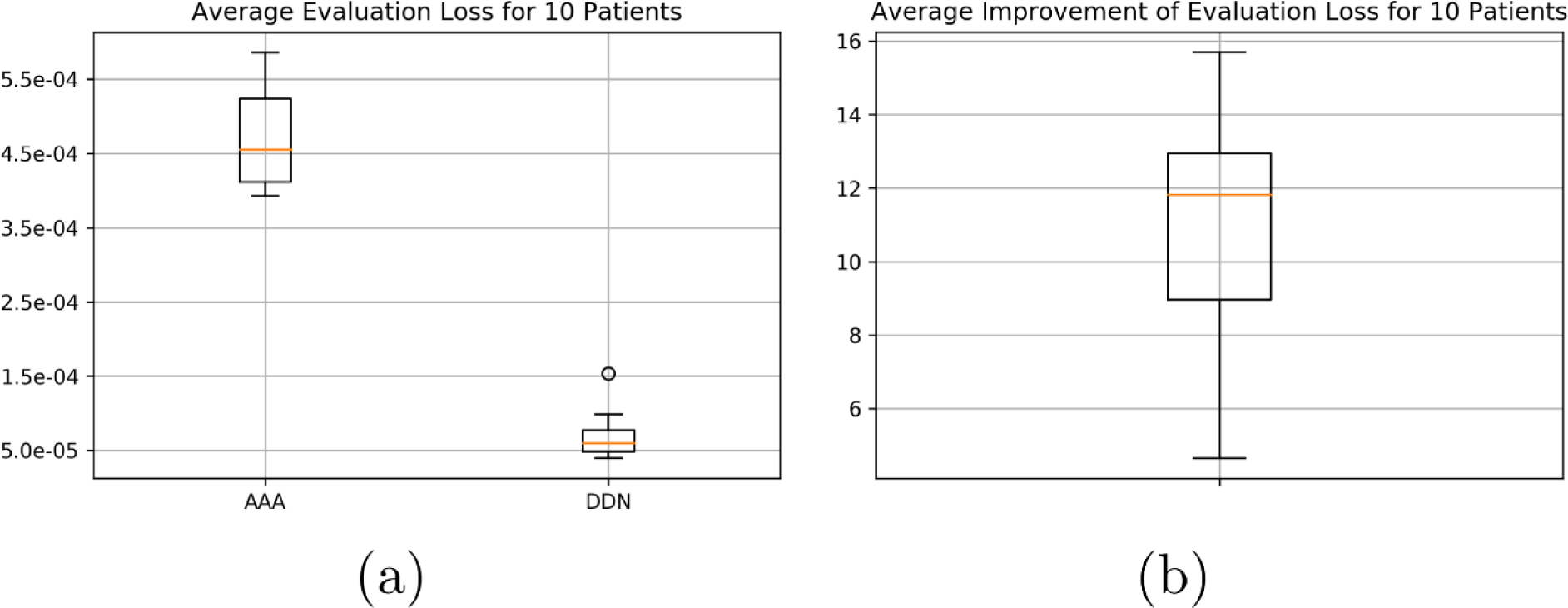
(a) Box plots for the average evaluation loss for 10 patients between AAA and DDN when compared with AXB. (b) Average improvement of evaluation loss for 10 patients.

We linearly interpolated the AAA dose distribution of 5 mm pixel size to 1.25 mm resolution. For each of the 10 models, the up-sampled dose distribution was compared with the AXB calculation with 1.25 mm resolution using 2D Gamma analysis for each slice. The same was performed for the DDN-derived dose distribution. We found that the average Gamma index passing rate at 3mm3% improved from 76% between the upsampled AAA and AXB to 91% between the DDN and AXB, from 66% to 86% at 2mm2%, and from 40% to 70% at 1mm1%. For the brain case, the 3mm3% passing rate improved from 69.9% to 89.0%, and for the pelvis case, 77.7% to 91.9%. The average calculation time of DDN was less than 1 milliseconds for a single slice. Fig. 6a shows the boxplot summarizing the above statements and Fig. 6b shows the violin plot of the gamma passing rate for the three different gamma indices.

Fig 6.

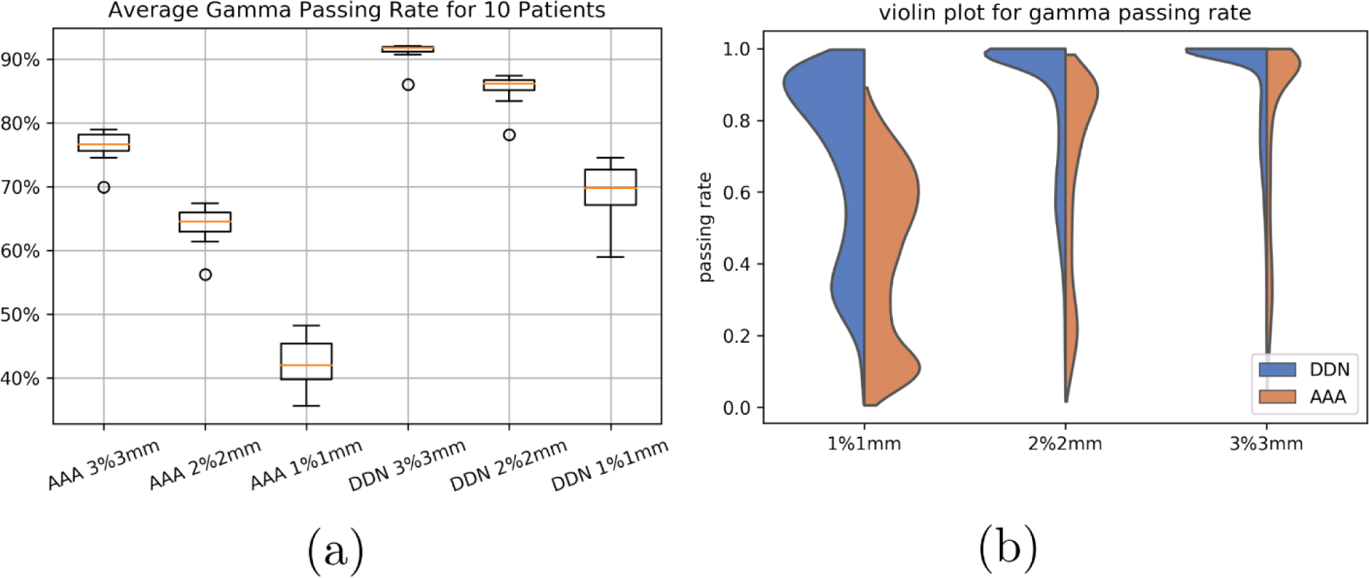
Gamma passing rate of the AAA and DDN methods as compared with that of the AXB at 1%1mm, 2%2mm, and 3%3mm. DDN method achieves markedly improved results.

It is also intriguing that, as can be seen from Fig. 7, the DDN inference yields sharper beam edges as compared with that of AAA. The results are more consistent with the AXB calculations. Moreover, the DDN also reconciles the tissue density heterogeneities along the beam path and adjusts the dose accordingly. In general, a better agreement between the AXB and DDN calculations in the low-density lung regions and in the high-density bones is clearly demonstrated in Fig. 7.

Fig 7.

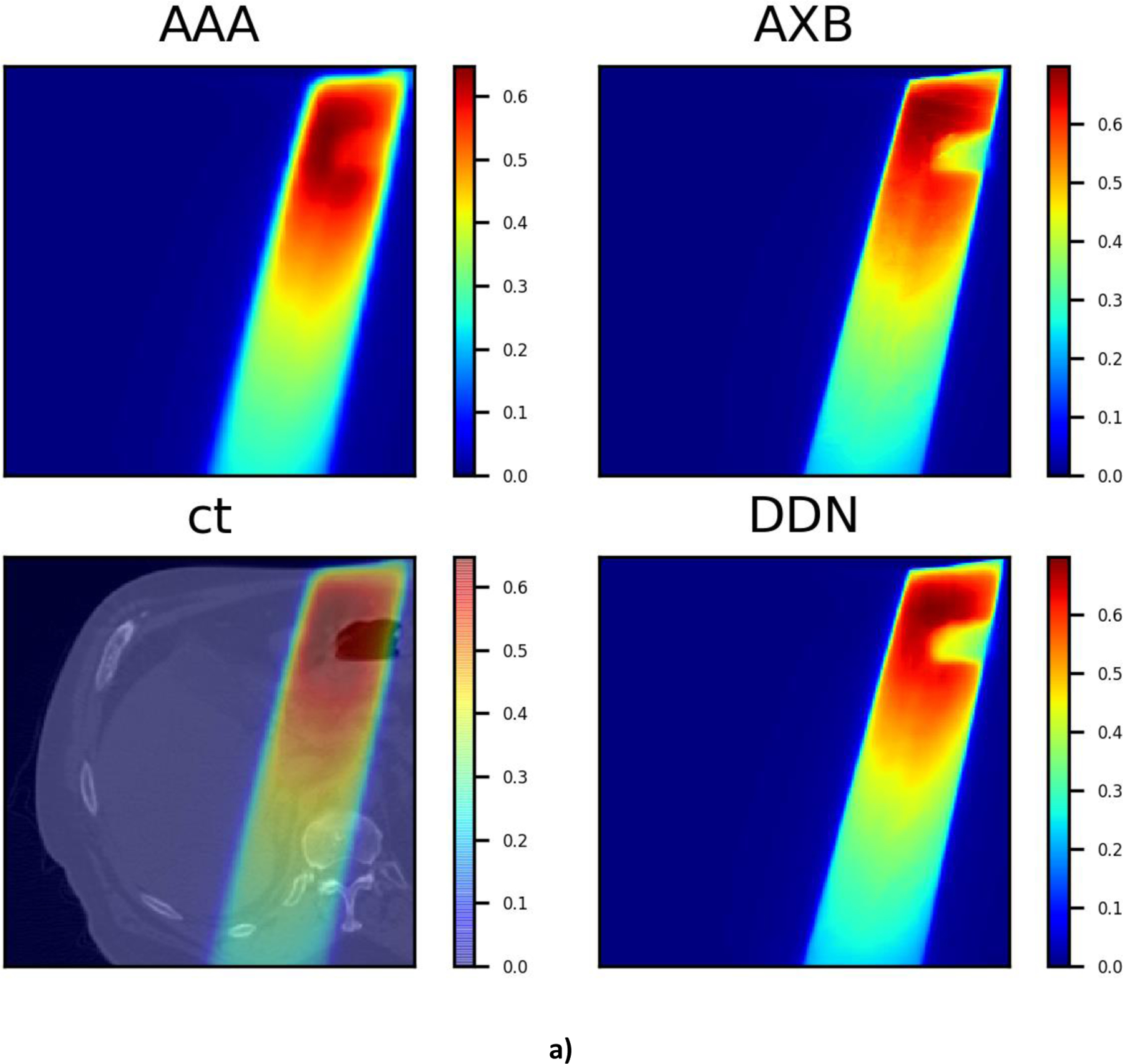
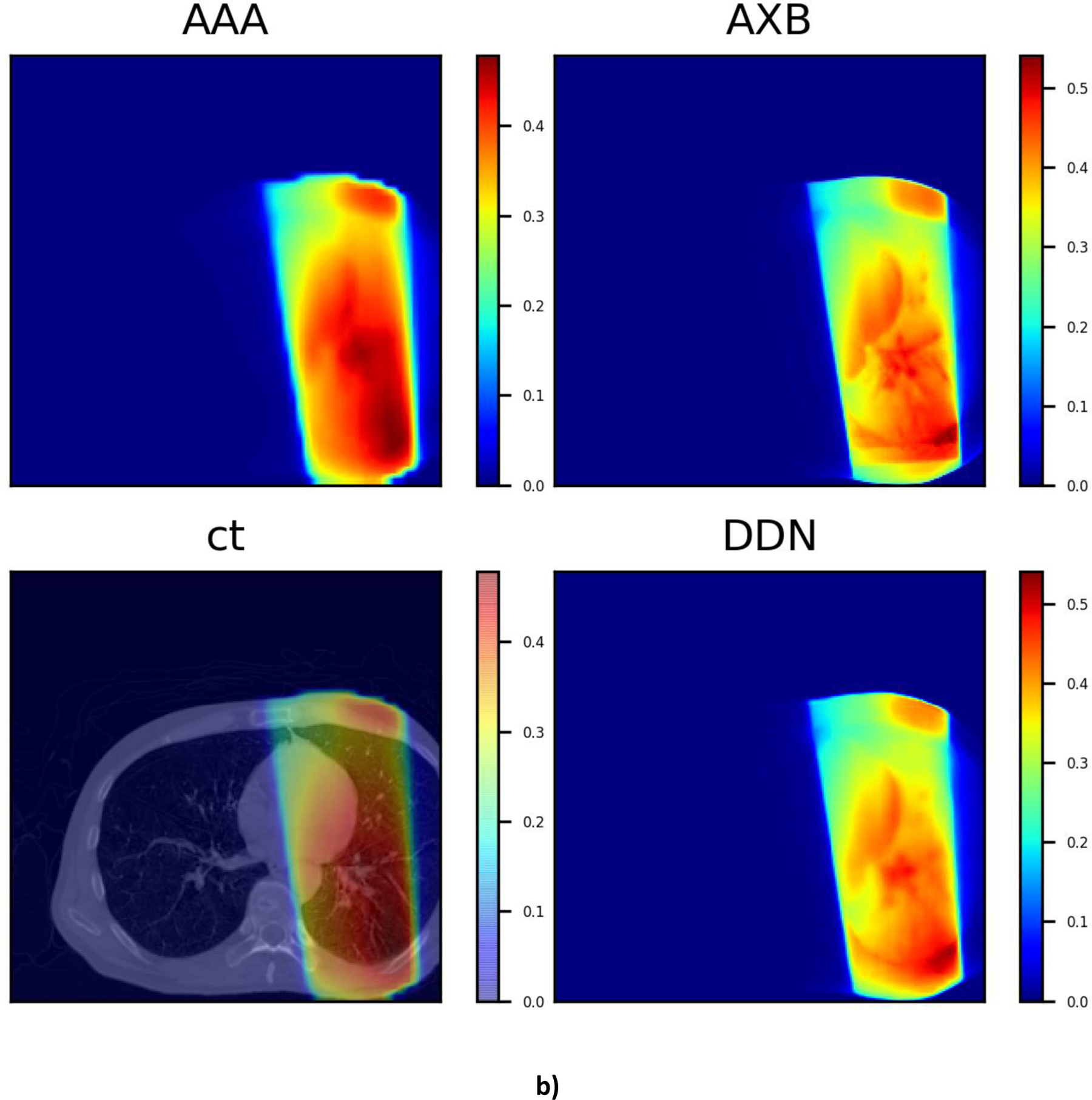
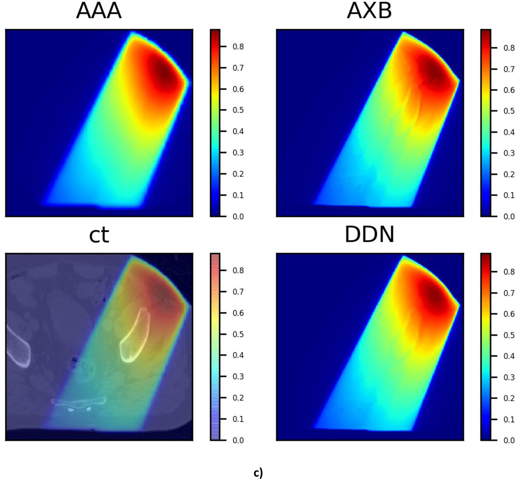
Three typical dose distributions in the validation study obtained using the DDN. For visualization/comparison, the AAA dose overlaid on CT, AAA and AXB doses are also displayed.

On average, it takes ~5 hours to calculate the 1.25 mm resolution AXB dose for 100 radiation therapy beams on our clinical 7 xenon servers with 6–8 cores each. The same calculations using AAA algorithm takes about 3 minutes when a pixel size of 5mm is selected. The proposed DDN method presents orders of magnitude improvement in computational efficiency with only limited (and controllable) compromise in the accuracy of resultant dose distribution. Indeed, the DDN super-resolution calculation for the same 100 beams would take only several seconds. The longer AXB calculation time is partly due to the inefficiency of the AXB algorithm to calculate the field dose rather than the plan dose. The plan dose calculation treats multiple fields in a plan as a whole and it’s not possible to get the dose contribution from each field separately, while the field dose option calculates each field in a plan independently. Ideally, we should compare with the performance of the AXB algorithm on a GPU, however, we don’t have access to one of the GPU systems. There are published data showing a speed up of 4.4 times for a GPU AXB implementation, which can have memory problems for field areas of 300 cm∧2 or below 0.15 cm grid resolution[31].

4. Discussions

The problem of single image super resolution is generally ill posed [32], with multiple solutions for the low-resolution image. Thus, the approach cannot be directly applied to dose super resolution. Effective incorporation of CT information into the DDN helps to alleviate the problem and facilitate the dose transformation calculation. In DDN, the CT image and low-resolution dose distribution are fed into the neural network simultaneously. Note that the CT information is reintroduced at each layer of the network, forcing the network to learn from CT when forming feature maps. The examples shown in Fig. 7 suggest that the DDN picks up the missing density information from the CT images. Generally, a high-performance image super resolution network structure would work better for the DDN with inclusion of the CT information.

We noticed that the evaluation losses for brain and pelvis cases are slightly worse than other sites, presumably due to less abundant training datasets with similar anatomies. By including more training data with more anatomical scenarios included, the performance of DDN is expected to improve. As shown in Fig. 8, the evaluation loss for a lung case improves steadily as more patients are included in the training dataset.

Fig. 8.

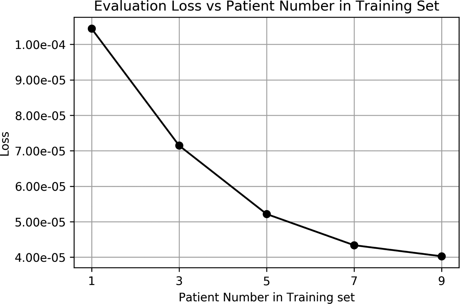
The loss function value as a function of the number of patients in the training datasets.

Our study here is focused on beams with an energy of 10FFF. Compared to lower energy beams, larger discrepancy has been reported between the doses calculated by AAA and AXB [33]. In reality, it is required to train a separate model for each energy. However, the procedure presented in the above is quite broad and generally applicable to any other beam energy or even other modality such as proton therapy and brachytherapy. A study of using super resolution dose approach for proton therapy is still in progress and will be reported in the future.

While the speed of current dose calculation algorithms is improving steadily over the years, the development seems to be outpaced by the increasing demands for higher spatial resolution for SBRT/SRS and treatment of small lesions such as oligomets and for the emerging plan optimization techniques such as MCO and robust optimization. Our study has clearly shown that significant acceleration of dose calculation is achievable by up-sampling the dose with deep learning techniques. The data-driven DDN provides an efficient tool for obtaining accurate dose distribution with high spatial resolution without paying the widely recognized overhead associated with the high-performance dose computing. Finally, we note that the DDN is not yet a full-fledged dose calculation engine. Future directions of improvement might include inferring from 3D CT and AAA data directly, expanding the training dataset to include more CTs, including more beams with different energies and machines, and replacing AAA dose with a simple ray tracing to further speed up the total dose calculation.

5. Conclusion

We have proposed a novel deep learning strategy to obtain highly accurate dose plan by transforming from a dose distribution calculated using a low-cost algorithm or algorithmic setting. Although the feasibility of the approach is demonstrated by using AAA and AXB, the method is quite general and can easily be applied to other algorithms, such as Monte Carlo based calculations. It is important to emphasize that the speed of the DDN does not depend on the algorithm it mimics, only the resolution. This makes it an ideal acceleration add-on for any dose calculation engine to speed up the treatment planning process. Dose super resolution represents a fertile area of research and development in medical physics to harness the enormous potential of deep learning.

Fig. 2.

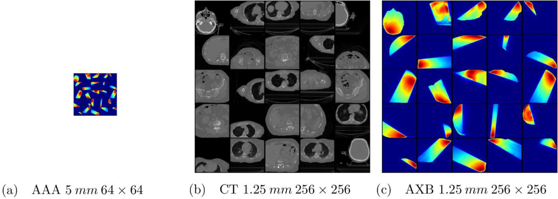
Examples of training data for DDN. (a) AAA dose map with a resolution of 5 mm and a size of 64×64. (b) Corresponding CT images with a resolution of 1.25 mm and a size of 256×256. The images are truncated from the original 512×512 images to save computing memories and speed up calculation. (c) The corresponding AXB dose map with a resolution of 1.25 mm and a size of 512×512. The size of the (a) is a quarter of the (b) and (c).

Fig. 3.

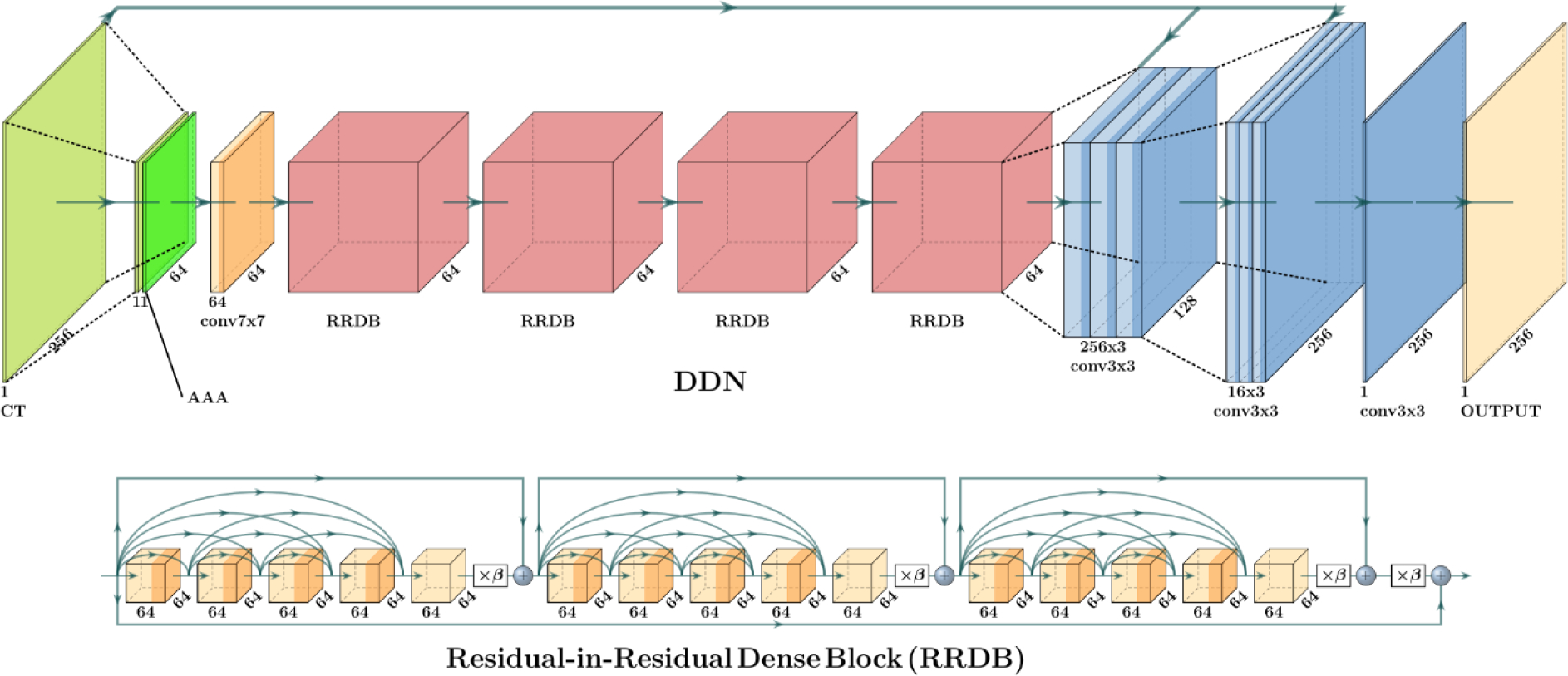
Deep DoseNet Structure. The top picture shows the DDN structure which starts from the downsampled CT and AAA dose, then continues with 64 7×7 filters, 4 RRDB blocks represented by red blocks, followed by two stage upsampling and final output. The bottom picture shows the detailed the RRDB block.

References

- [1].Onishi H et al. , “Stereotactic Body Radiotherapy (SBRT) for Operable Stage I Non-Small-Cell Lung Cancer: Can SBRT Be Comparable to Surgery?,” Int. J. Radiat. Oncol, vol. 81, no. 5, pp. 1352–1358, Dec. 2011. [DOI] [PubMed] [Google Scholar]
- [2].Lutz W, Winston KR, and Maleki N, “A system for stereotactic radiosurgery with a linear accelerator,” Int. J. Radiat. Oncol, vol. 14, no. 2, pp. 373–381, Feb. 1988. [DOI] [PubMed] [Google Scholar]
- [3].Mutic S and Dempsey JF, “The ViewRay System: Magnetic Resonance-Guided and Controlled Radiotherapy,” Semin. Radiat. Oncol, vol. 24, no. 3, pp. 196–199, Jul. 2014. [DOI] [PubMed] [Google Scholar]
- [4].Mackie TR, Scrimger JW, and Battista JJ, “A convolution method of calculating dose for 15-MV x rays,” Med. Phys, vol. 12, no. 2, pp. 188–196, 1985. [DOI] [PubMed] [Google Scholar]
- [5].Craft DL, Hong TS, Shih HA, and Bortfeld TR, “Improved Planning Time and Plan Quality Through Multicriteria Optimization for Intensity-Modulated Radiotherapy,” Int. J. Radiat. Oncol, vol. 82, no. 1, pp. e83–e90, Jan. 2012. [DOI] [PMC free article] [PubMed] [Google Scholar]
- [6].Chu M, Zinchenko Y, Henderson SG, and Sharpe MB, “Robust optimization for intensity modulated radiation therapy treatment planning under uncertainty,” Phys. Med. Biol, vol. 50, no. 23, pp. 5463–5477, Nov. 2005. [DOI] [PubMed] [Google Scholar]
- [7].Dong P, Liu H, and Xing L, “Monte Carlo tree search -based non-coplanar trajectory design for station parameter optimized radiation therapy (SPORT),” Phys. Med. Biol, vol. 63, no. 13, p. 135014, Jul. 2018. [DOI] [PubMed] [Google Scholar]
- [8].Andreo P, “Monte Carlo techniques in medical radiation physics,” Phys. Med. Biol, vol. 36, no. 7, pp. 861–920, Jul. 1991. [DOI] [PubMed] [Google Scholar]
- [9].Rogers DWO, Faddegon BA, Ding GX, Ma C-M, We J, and Mackie TR, “BEAM: A Monte Carlo code to simulate radiotherapy treatment units,” Med. Phys, vol. 22, no. 5, pp. 503–524, 1995. [DOI] [PubMed] [Google Scholar]
- [10].Failla GA, Wareing T, Archambault Y, and Thompson S, “Acuros XB advanced dose calculation for the Eclipse treatment planning system,” Palo Alto CA Varian Med. Syst, vol. 20, 2010. [Google Scholar]
- [11].LeCun Y, Bengio Y, and Hinton G, “Deep learning,” Nature, vol. 521, no. 7553, pp. 436–444, May 2015. [DOI] [PubMed] [Google Scholar]
- [12].Xing L, Krupinski EA, and Cai J, “Artificial intelligence will soon change the landscape of medical physics research and practice,” Med. Phys, vol. 45, no. 5, pp. 1791–1793, 2018. [DOI] [PMC free article] [PubMed] [Google Scholar]
- [13].Szegedy C, Ioffe S, Vanhoucke V, and Alemi A, “Inception-v4, Inception-ResNet and the Impact of Residual Connections on Learning,” ArXiv160207261 Cs, Feb. 2016.
- [14].Fauw JD et al. , “Clinically applicable deep learning for diagnosis and referral in retinal disease,” Nat. Med, vol. 24, no. 9, p. 1342, Sep. 2018. [DOI] [PubMed] [Google Scholar]
- [15].Ronneberger O, Fischer P, and Brox T, “U-net: Convolutional networks for biomedical image segmentation,” in International Conference on Medical image computing and computer-assisted intervention, 2015, pp. 234–241. [Google Scholar]
- [16].Dong C, Loy CC, He K, and Tang X, “Image Super-Resolution Using Deep Convolutional Networks, ” IEEE Trans. Pattern Anal. Mach. Intell, vol. 38, no. 2, pp. 295–307, Feb. 2016. [DOI] [PubMed] [Google Scholar]
- [17].Liu H, Xu J, Wu Y, Guo Q, Ibragimov B, and Xing L, “Learning deconvolutional deep neural network for high resolution medical image reconstruction, ” Inf. Sci, vol. 468, pp. 142–154, 2018. [Google Scholar]
- [18].Gatys LA, Ecker AS, and Bethge M, “Image style transfer using convolutional neural networks, ” in Proceedings of the IEEE conference on computer vision and pattern recognition, 2016, pp. 2414–2423. [Google Scholar]
- [19].Ma M, Kovalchuk N, Buyyounouski MK, Xing L, and Yang Y, “Dosimetric features-driven machine learning model for DVH prediction in VMAT treatment planning, ” Med. Phys, vol. 46, no. 2, pp. 857–867, 2019. [DOI] [PubMed] [Google Scholar]
- [20].Ma M, Buyyounouski MK, Vasudevan V, Xing L, and Yang Y, “Dose distribution prediction in isodose feature-preserving voxelization domain using deep convolutional neural network, ” Med. Phys, vol. 46, no. 7, pp. 2978–2987, 2019. [DOI] [PubMed] [Google Scholar]
- [21].Dong P and Xing L, “DoseNet: A Deep Neural Network for Accurate Dosimetric Transformation Between Different Spatial Resolutions And/or Different Dose Calculation Algorithms for Precision Radiation Therapy, ” in MEDICAL PHYSICS, 2019, vol. 46, pp. E473–E473. [DOI] [PMC free article] [PubMed] [Google Scholar]
- [22].Kim J, Lee JK, and Lee KM, “Accurate Image Super-Resolution Using Very Deep Convolutional Networks, ” ArXiv151104587 Cs, Nov. 2015.
- [23].Ledig C et al. , “Photo-Realistic Single Image Super-Resolution Using a Generative Adversarial Network, ” ArXiv160904802 Cs Stat, Sep. 2016.
- [24].He K, Zhang X, Ren S, and Sun J, “Deep Residual Learning for Image Recognition, ” ArXiv151203385 Cs, Dec. 2015.
- [25].Radford A, Metz L, and Chintala S, “Unsupervised Representation Learning with Deep Convolutional Generative Adversarial Networks, ” ArXiv151106434 Cs, Nov. 2015.
- [26].Han T, Mikell JK, Salehpour M, and Mourtada F, “Dosimetric comparison of Acuros XB deterministic radiation transport method with Monte Carlo and model-based convolution methods in heterogeneous media, ” Med. Phys, vol. 38, no. 5, pp. 2651–2664, May 2011. [DOI] [PMC free article] [PubMed] [Google Scholar]
- [27].Wang X et al. , “Esrgan: Enhanced super-resolution generative adversarial networks, ” in Proceedings of the European Conference on Computer Vision (ECCV), 2018, pp. 0–0. [Google Scholar]
- [28].He K, Zhang X, Ren S, and Sun J, “Delving deep into rectifiers: Surpassing human-level performance on imagenet classification, ” in Proceedings of the IEEE international conference on computer vision, 2015, pp. 1026–1034. [Google Scholar]
- [29].Le QV, Ngiam J, Coates A, Lahiri A, Prochnow B, and Ng AY, “On optimization methods for deep learning, ” in Proceedings of the 28th International Conference on International Conference on Machine Learning, 2011, pp. 265–272. [Google Scholar]
- [30].Abadi Martin et al. , TensorFlow: Large-Scale Machine Learning on Heterogeneous Systems. 2015.
- [31].Aland T, Walsh A, Jones M, Piccini A, and Devlin A, “Accuracy and efficiency of graphics processing unit (GPU) based Acuros XB dose calculation within the Varian Eclipse treatment planning system, ” Med. Dosim. Off. J. Am. Assoc. Med. Dosim, vol. 44, no. 3, pp. 219–225, Autumn 2019. [DOI] [PubMed] [Google Scholar]
- [32].Yang J, Wright J, Huang TS, and Ma Y, “Image super-resolution via sparse representation, ” IEEE Trans. Image Process, vol. 19, no. 11, pp. 2861–2873, 2010. [DOI] [PubMed] [Google Scholar]
- [33].Huang B, Wu L, Lin P, and Chen C, “Dose calculation of Acuros XB and Anisotropic Analytical Algorithm in lung stereotactic body radiotherapy treatment with flattening filter free beams and the potential role of calculation grid size,” Radiat. Oncol, vol. 10, no. 1, p. 53, Feb. 2015. [DOI] [PMC free article] [PubMed] [Google Scholar]