

Abstract
This study predicts the number of visitors to an international tourism Expo to be held in Korea in 2012, an unprecedented event for the host city. Forecasting demand for such a mega-event has received only limited attention in the literature. Unlike most studies forecasting international tourism demand, forecasting Expo demand involves using both quantitative forecasting models and qualitative technique because of data limitations. Combining quantitative techniques with willingness-to-visit (WTV) surveys predicts the Expo demand at 8.9 million visitors. In comparison using the Delphi method, experts predict Expo demand at 6.8 million visitors. For this study, the Delphi method provides more conservative estimates than estimates from combining quantitative techniques with WTV. Policy implications presented are directed toward Expo planners and practitioners in terms of demand and supply side, application of these results in the decision-making process, and future challenges surrounding demand forecasting.
Keywords: Expo, Demand forecasting, Seasonal ARIMA intervention, Winters, Regression, Delphi, Willingness-to-visit
1. Introduction
Interest in mega-events, such as Expos, the World Cup, and the Olympics, is increasing for numerous reasons including their contribution to tourism (Green & Chalip, 1998; Lee, Lee, & Wicks, 2004). Mega-events’ effects on host countries include increased tourist receipts, income, employment, government revenues, and cultural awareness, along with an improved image of the country (Lee, Lee, & Lee, 2005). To realize these positive effects, however, host countries experience high infrastructure development and other costs. Getz (1991) recognizes festivals and events as a new wave of alternative tourism, contributing to sustainable development and improving the relationships between hosts and guests.
Forecasting tourism demand helps both the public and private sectors improve the allocation of scarce resources (Quayson & Var, 1982), which plays a vital role in avoiding shortages or surpluses in the tourism sector (Burger, Dohnal, Kathrada, & Law, 2001). Investments in tourism infrastructures require huge financial commitments from both the public and private sectors. More accurate forecasts provide better estimates of expected return on investments, which help guide investment decisions (Song & Witt, 2006). Specifically, forecasting demand for an international tourism Expo is not only important in the bidding process among international competitors, but also is necessary to help gain public support for hosting the mega-event and determine the expected benefits and costs associated with hosting the event. In the planning stage, forecasting tourism demand is prerequisite to determine factors impacting investment decisions such as the capacity of the Expo site and facilities, necessary road and transportation system expansions, and appropriate food and lodging facilities. Accurate forecasts of tourism demand, therefore, not only help the event planners ensure the successful hosting of an Expo, but also provide them with considerable information to guide their investment decisions (Lee, 1996).
Yeosu City, South Korea with support from the Korean government proposed to host the International Marine Expo for 3 months in the year 2012, which is organized by Bureau International des Expositions (BIE). In spite of the plethora of research on demand forecasting, little research has been conducted on forecasting tourism demand for such an Expo. Because most international Expos are a one-time event, past quantitative data are very limited, increasing the difficulty in predicting Expo demand. The current study provides a methodology that combines different approaches based on available data to overcome the lack of data. Forecasts of the number of tourists visiting the Yeosu International Marine Expo are obtained by combining quantitative techniques with willingness-to-visit (WTV) obtained from survey data.
Demand for the Expo is broken into potential number of visitors by international tourists and domestic tourists by adult and adolescents. International tourist demand is estimated by combining forecasts of international tourist demand based on historical data with survey data on WTV. Before quantitative methods are combined with WTV from the survey, several different quantitative time-series forecasting models of international tourist arrivals are estimated and evaluated. A range of forecasts is obtained using the different methods to provide a richer view of the potential demand for the Expo. Domestic demand is based on WTV derived from a survey and population projections. Forecast of total domestic and international visitors from these methods are then compared to an estimate obtained from experts using the Delphi method.
2. Review of forecasting techniques
A variety of forecasting techniques have been used to estimate tourism demand. The appropriate methods used to forecast tourism demand vary depending on data availability, time horizons, and objectives. Strengths and weaknesses of the various methods have been comprehensively reviewed (Calantone, Di Benedetto, & Bojanic, 1987; Crouch, 1994; Li, Song, & Witt, 2005; Lim, 1997; Uysal & Cromption, 1985; Var & Lee, 1993). Methodologies used to forecast tourism demand are broadly classified into quantitative and qualitative approaches (Calantone et al., 1987; Crouch, 1994; Lim (1997), Lim (1999); Uysal & Cromption, 1985; Var & Lee, 1993).
2.1. Quantitative forecasting techniques
Quantitative techniques are used for forecasting tourism demand when information on past tourism can be quantified and past patterns can reasonably be assumed to continue into the future (Makridakis & Wheelwright, 1978). Two main quantitative approaches used are time series and causal or explanatory models. Time-series models use historical data patterns to generate future forecasts. Commonly used time-series models in tourism research are exponential smoothing (Burger et al., 2001; Geurts & Ibrahim (1975), Geurts & Ibrahim (1982); Lim & McAleer, 2001) and autoregressive integrated moving average (ARIMA) models (Burger et al., 2001; Cho, 2003; Goh & Law, 2002; Kim & Moosa, 2005; Kulendran & Witt (2003a), Kulendran & Witt (2003b); Li et al., 2005; Lim, 2002; Lim & McAleer, 2002).
Geurts and Ibrahim (1975) compared a Box–Jenkins (ARIMA) model with a Brown exponential smoothing model in the context of Hawaiian tourism demand. Results indicate that both the Box–Jenkins and the exponential smoothing models performed equally well in terms of forecasting accuracy, but the latter may be preferred because it is easier to use. Geurts and Ibrahim (1982) demonstrate that the forecasting accuracy of Hawaiian tourism was greatly improved after accounting for atypical months and if the forecasts were updated annually. Burger et al. (2001) compared naïve, moving average (MA), ARIMA, decomposition, and exponential smoothing time-series models in forecasting the US demand for travel to Durban, South Africa. They indicate that in terms of accuracy the exponential smoothing model performed best, followed by naïve, ARIMA, and MA models. The decomposition method performance was inferior to the other models. Lim and McAleer (2001) show the Holt-Winters seasonal exponential smoothing models outperformed both the single and double exponential smoothing models in predicting tourist arrivals to Australia. Lim (2002) employed ARIMA models to forecast international tourism demand for Australia. Their results show that the ARIMA models outperformed the seasonal ARIMA models for forecasting demand from Hong Kong and Malaysia tourists, but demand from Singapore tourists was better forecasted using the seasonal ARIMA model. Goh and Law (2002) found that ARIMA models with seasonality and interventions performed better than other time-series models, because the ARIMA Intervention model reflected the impacts from special events. Cho (2003) predicted tourism demand from different countries to Hong Kong using three time-series models, exponential smoothing, ARIMA, and artificial neural networks. Results indicate the artificial network model outperformed the smoothing and ARIMA models. Cho (2003), however, suggested that ARIMA and smoothing models were also sufficiently adequate for forecasting tourism demand. Kulendran and Witt (2003b) indicate the ARIMA model was more accurate than the error correction model (ECM) for short-term forecasts; however, the ECM outperformed the ARIMA for long-term forecasts.
Causal or explanatory models are based on the assumption that the factor being forecast has a cause-and-effect relationship with one or more variables. Economic-based causal models have been used in forecasting tourism demand (Song & Witt, 2006), particularly when identifying important explanatory variables affecting international tourism demand is an objective (Crouch, 1994; Lim, 1999; Uysal & Cromption, 1984). Income is often identified as the single most important determinant of international tourism demand (Artus, 1972; Barry & O’Hagan, 1972; Crouch, 1994; Di Matteo & Di Matteo, 1993; Gray, 1966; Jud & Joseph, 1974; Laber, 1969; Lee, 1996; Lee, Var, & Blaine, 1996; Loeb, 1982; Sheldon, 1993; Stronge & Redman, 1982; Uysal & Cromption, 1984; Witt & Martin, 1987). Relative prices are also found to be significant as a determinant of demand for international tourism (Barry & O’Hagan, 1972; Crouch, 1992; Han, Durbarry, & Sinclair, 2006; Lee et al., 1996; Loeb, 1982; Quayson & Var, 1982; Uysal & Cromption, 1984; Witt & Witt, 1990). Other variables such as exchange rate (Artus, 1972; Gerakis, 1965; Lee et al., 1996; Uysal & Cromption, 1984) and marketing aspects (Barry & O’Hagan, 1972; Crouch, 1994; Lee, 1996; Uysal & Cromption, 1984) are often found to be significant explanatory variables.
Li et al. (2005) observed recent development in econometric models based on overview of past research in terms of model specifications, major determinants, and test of forecasting accuracy. They suggest increased understanding of international tourism demand could be achieved by applying advanced econometric models, such as time-varying parameter (TVP) models (Li, Wong, Song, & Witt, 2006), vector autoregressive (VAR) models (Song & Witt, 2006), Bayesian VAR (Wong, Song, & Chon, 2006), and almost ideal demand systems (AIDS) (Han et al., 2006).
Unfortunately, no one quantitative method has been shown to be superior to the other techniques. Data availability, study objectives, and situation being studied all play a significant role in determining which method is the most appropriate.
2.2. Qualitative forecasting techniques
Qualitative techniques are used for forecasting tourism demand when changes of a large and unprecedented nature are likely to occur, examples of such changes would be mega-events. Qualitative techniques include the Delphi method, which was first applied by Dalkey and Helmer (1963). Being dependent upon the accumulated experience of experts, this method assembles a panel of experts from disciplines to obtain a group consensus concerning the likely outcome of future events (Archer, 1987). This method assumes that the range of responses will decrease as convergence is achieved toward the midrange of the distribution (Kaynak & Macaulay, 1984). One example of the use of the Delphi model is Liu (1988). Liu predicted Hawaiian tourism demand for 2000 using two separate panels, local tourist receivers and overseas tourist senders. Forecasts of tourism demand made by both local and outside experts were generally consistent with state projections. Lee and Kim (1998) also used the Delphi model for predicting international tourism demand for World Cup games in Korea. Forecasts made by the panel members were 456,000 attendees to the 2002 World Cup which is slightly higher than the actual tourists arrivals of 403,000 (Korea National Tourism Organization, 2006) during the World Cup.
Prideaux, Laws, and Faulkner (2003) assert that qualitative methods such as Delphi are useful because quantitative techniques such as time-series and econometric models use historical data that may not contain information on future events, thus their uncertainty in the future. Qualitative forecasting techniques such as the Delphi model are particularly suitable for long-term forecasting when changes of a large and unprecedented nature are taken into consideration by forecasting experts (Archer, 1987; Liu, 1988; Var & Lee, 1993).
2.3. Accuracy as a criterion for selecting forecasting model
Choosing the most appropriate forecasting model depends heavily on the forecasting situation, such as data patterns, time horizon, costs, and ease of application (Var & Lee, 1993). Accuracy is frequently the criterion used for selecting the “best” forecasting model (Burger, et al., 2001; Li et al., 2005; Lim & McAleer, 2002). Empirical studies show that forecasts from complex and statistically sophisticated methods are not necessarily more accurate than forecasts from relatively simple methods (Makridakis, 1986; Lim & McAleer, 2002). Martin and Witt (1989) indicate that econometric models may not be more accurate than time-series models in terms of forecasts. Van Doorn (1984) maintains that the use of simple forecasting models proved more accurate than complex models. Ascher (1978, p. 199) also observed, “The presumed advantages of sophisticated methodologies simply have not materialized.” For this reason, Calantone et al. (1987) stressed that complex model building should not be undertaken for its own sake. Li et al. (2006) correctly assert that there is no single forecasting model that performs better than the others in all cases because many factors influence forecasting performance. Although many studies indicate that relatively simple methods often outperform sophisticated or complex models, debate on the performance between simple and complex models in terms of forecasting accuracy is still ongoing.
To determine forecasting accuracy, frequently used measures include mean square error (MSE), root mean square error (RMSE), and mean absolute percentage error (MAPE). The primary limitation of MSE is that it does not facilitate comparisons across different time series or over different time intervals, because it is an absolute measure (Makridakis, Wheelwright, & Victor, 1983). RMSE has also limitation in terms of less intuitive (Ascher, 1978). MAPE has been preferred by many researchers (Burger et al., 2001; Cho, 2003; Chu, 1998; Kulendran & Witt, 2003b; Song & Witt, 2006; Wheelwright & Makridakis, 1985), because it is expressed as a percentage of actual values over predicted values. Lewis (1982) suggests the following interpretation of the MAPE statistic: highly accurate forecasts are associated with the model if the MAPE is less than or equal to 10%; good forecasts for MAPE=10–20%; reasonable forecasting for MAPE=20–50%; and inaccurate forecasting for greater than MAPE=50%. MAPE is calculated by the following equation:
| (1) |
where Xi is the actual data for period i; Fi the forecast for period i; | | represents absolute value; and n the number of observations.
In this study, the MAPE is used for measuring accuracy and is the criterion used for selecting the most appropriate forecasting model for tourism demand among the quantitative techniques employed.
3. Methodology
Demand for the Expo consists of international inbound tourists (hereafter foreign tourists) and domestic visitors, which are broken down into adult and adolescent visitors. Specific forecasting procedures are described for each of these groups.
3.1. Forecasting the Expo demand for foreign tourists
Expo demand for foreign tourists is predicted using two steps. In the first step, foreign tourists in the year of 2012 are predicted by using time-series models based on quarterly tourist data from 1990 to 2005 published by Korean National Tourism Organization (2006). Three time-series models, seasonal ARIMA (SARIMA) Intervention, Winters, and Trend Regression model, are used to forecast foreign tourists demand for the Expo. The SARIMA Intervention model incorporates seasonal fluctuations, as well as, the impacts of the following events, IMF (Asian Financial) Crisis, 9/11 terrorism, FIFA World Cup, and Severe Acute Respiratory Syndrome (SARS). Using three levels of smoothing, the Winters model is estimated to represent smoothing type models. Finally, the Trend model, which also includes variables for the impact of the above events, represents one of the simplest possible model formulations. In the second step, WTV is estimated from an on-site survey for foreign tourists (see Survey design and data collection section). Finally, Expo demand by foreign tourists is forecasted by multiplying predicted number of foreign tourists by the WTV estimated from the survey data.
3.1.1. Seasonal ARIMA Intervention model
The autoregression (AR) model is one in which the time-series variable is a function of past values of the variable. In a MA model, the time series is defined by past values of the error term. Combining the AR representation with the MA component one obtains the autoregressive moving average (ARMA) model. Because the ARMA model requires stationary data, non-stationary data are differenced (integrated) to make the data stationary (Makridakis, Wheelwright, & Hyndman, 1998). In this case, model becomes the ARIMA model. Non-stationarity indicates that mean and variance of a series are not constant through time and autocovariance of the series is time varying (Enders, 1995). Taking into account seasonality the model becomes a SARIMA.
Time-series data are often influenced by exogenous or external events. Such exogenous events, called interventions (Glass, 1972), increase the difficult in developing forecasting models. Incorporating these interventions often improves the accuracy of generated forecasts and provides a measure of the impact of the interventions (Box & Tiao, 1975). Empirical studies, such as Goh and Law (2002), show ARIMA Intervention models, which are an extension of the univariate Box–Jenkins ARIMA models, often perform well.
Consider a stationary (integrated of order d) time series, Yt and m number of interventions, the SARIMA Intervention model can be expressed as (Enders, 1995):
| (2) |
where C is the constant term; Xi,t the deterministic binary dummy variable with 0 and 1; ai the magnitude of intervention (Xi,t); and Nt the stochastic disturbance assumed to be SARIMA model.
The disturbance term can be expressed in the following form:
| (3) |
where B is the backshift or one period lag operator; d the d-order non-seasonal difference operator; D the D-order seasonal difference operator; φp(B) the p-order non-seasonal AR model; ΦP(B S): P-order seasonal AR model; θq(B) the q-order non-seasonal MA model; ΘQ(B) the Q-order seasonal MA model; and et the error term ∼IID (0, σ 2).
Assuming multiplicative seasonality, the time structure of Nt is given by a general SARIMA (p,d,q) (P,D,Q) process. The error term is assumed to have a zero mean, constant variance, and be serially uncorrelated (Enders, 1995; Nelson, 2000).
The effects of interventions can be for a single period or spread over a multi periods. The former is called a pulse, while the letter is called a step. In this study, a qualitative zero–one dummy variable is used to represent the effect of interventions. The specific time when the interventions influence tourist arrivals is determined based on prior knowledge of the intervention and by visual examination of the data (Fig. 1 ). A one-pulse function is used for the 2002 FIFA World Cup of Korea–Japan (2nd quarter of 2002). Multi-period functions are used for the IMF (Asian Financial) Crisis (4th quarter of 1997 through 3rd quarter of 2001), 9/11 terrorism (3rd quarter of 2001 through 1st quarter of 2002), and SARS (2nd quarter of 2003 through 3rd quarter of 2003) (Lee & Taylor, 2005; WHO, 2003).
Fig. 1.

Quarterly foreign tourist arrivals to Korea and interventions.
3.1.2. Winters model
Winters model, one of the exponential smoothing methods, is particularly useful when data pattern exhibits seasonality. The Winters model consists of three smoothing equations: level, trend, and seasonality (Makridakis et al., 1998):
| (4) |
| (5) |
| (6) |
and
| (7) |
where Yt is the actual (observed) values; Lt the single smoothed values (the level of the series); bt the trend; St the seasonal component; s the length of seasonality; Ft+m the forecast for m period ahead; and α, β, γ are coefficients to be estimated that range from 0 to 1 and used to minimize mean squared errors.
3.1.3. Trend model
A quadratic trend model, which incorporates the same interventions as the SARIMA Intervention model, is estimated using ordinary least squares:
| (8) |
where Yt is the tourism demand; t the time period; D the dummy variables: D 1 the IMF (Asian Financial) Crisis, D 2 the 9/11 terrorism; D 3 the World Cup, and D 4 the SARS; βi and ri are coefficients to be estimated; and et the error term assumed to be independent and identically distributed.
3.2. Forecasting Expo demand for domestic visitors
3.2.1. Adult visitors
Because demand for the Expo may differ between origin and destination, depending on distance and other factors, demand is estimated for 16 regions (7 metropolitan cities and 9 provinces). To obtain Expo demand, projected population in 2012 is necessary. Forecasting population is not commonly the domain of the field of tourism, however, the Korea National Statistical Office specializes in the projection of domestic population using a cohort component method. As such, this study utilizes projected adult and adolescent populations in 2012 in the 16 regions obtained from the Korea National Statistical Office (2006a). Based on the traditional demographic accounting system, the cohort component predicts the components of population change by each cohort of the same age with respect to fertility, mortality, and net migration. With this cohort component method population at the next time period is projected based on a base population by age and sex, natural increase (births–deaths), and net migration as given in the following equation (Korea National Statistical Office, 2006a):
| (9) |
where Pt is the population at the beginning time period; Pt +1 the population at the next time period; I the natural increase (births–deaths); and M the net migration during the period.
Expo demand by the adult population for each region is predicted by multiplying projected adult population in 2012 by WTV:
| (10) |
where Yadult is the Expo demand for domestic adult visitors; Pi the projected adult population in the year of 2012 in region i; and Wi the WTV in region i.
To obtain WTV, a quota sampling survey (for details, see Survey design and data collection section) based on sex and age for the 16 regions is conducted.
3.2.2. Adolescent visitors
Expo demand for adolescent visitors is separately predicted because adolescents are generally accompanied by their parents. Expo demand by domestic adolescents is calculated using the following formula:
| (11) |
where Yadolescent is the Expo demand for domestic adolescent population; Pi the projected adult population in the year of 2012 in region i; Ai the percent of the population age 30–49 in region i; Wi the WTV in the region i; and Ni the number of adolescent to be accompanied by parents age 30–49 in the region i.
The proportion of parents accompanying adolescents and number of adolescents to be accompanied by parent are estimated using the data from Korean National Statistical Office (2006a), whereas, WTV is estimated based on the national survey data. According to Korean National Statistical Office (2006b), population age category of 30–49 is the most likely to have adolescents in their household. Therefore, this age group is assumed to be the group most likely to accompany adolescents attending the Expo. Finally, Expo demand for adolescent is predicted by multiplying projection of adolescent population by WTV of parents.
3.3. Survey design and data collection
3.3.1. Foreign tourists
Over 70% of international visitors to Korea are from Japan, China including Hong Kong, Taiwan, and the US. As such, the survey was directed toward tourists from these countries by providing the survey instrument in English, Japanese, and Chinese. However, tourists from Canada and Europe, representing additional 10% of total arrivals were also asked to participate. The first part of questionnaire included an introduction, describing purpose of the research, and information on the Expo. Respondents were then answered the question “Are you willing to visit the Expo if the City of Yeosu hosts it” using a 5-point Likert-type scale with 1 being very unlikely, 3 neutral, and 5 being very likely. The last part of the questionnaire ascertained demographic characteristics of the respondents, such as sex and age. On-site surveys of foreign tourists were conducted at the most popular tourist sites in Seoul including Duksoo and Kyungbok Palaces, Myungdong, and Insadong. The self-administered intercept survey was conducted by graduate students enrolled in a class on forecasting tourism demand. When possible, students fluent in Japanese and Chinese conducted the survey for Japanese and Chinese visitors, and students fluent in English conducted the survey for Americans and other English-speaking foreign visitors. The survey was administered on both weekdays and weekends during October and November 2005. A total of 429 usable questionnaires were collected during the survey.
As pointed out by a reviewer, a sample of future foreign tourists should be surveyed to obtain WTV. To survey potential future visitors, surveys would have to be conducted in the countries of origin. Time and cost limitations did not allow for such a design. In surveying only current foreign tourists and using their WTV, the assumption is made that current tourists’ WTV is representative of future tourists’ WTV.
3.3.2. Domestic visitors
A national survey was conducted to estimate national WTV the Yeosu Expo. Twenty-five hundred observations were proportionately allocated to 16 regions based on population size (Korea National Statistical Office, 2005). A quota sampling method for each region was employed according to age and sex based on national population statistics. The first part of questionnaire included an introduction, describing purpose of the research and information on the Expo. Next, respondents’ answered the question “Are you willing to visit the Expo if the City of Yeosu hosts it?” Two WTV questions were posed to the respondents. The first question assumed no admission fee, whereas, the second question included a fee of 20,000 Won (approximately US$ 21). In this study, the WTV based on the question including the admission fee is used to provide a conservative estimate of the number of visitors as this question provided a lower WTV. As in the foreign tourist survey, a 5-point Likert-type scale was used. The third part of the questionnaire determined the number of adolescent likely to accompany their parents to the Expo. Questions concerning demographic characteristics of respondents completed the questionnaire.
The survey was conducted on-site for 2 months from November to December 2005 in the 16 regions. Field researchers approached respondents in residential areas, outlined the purpose of the research project, and invited them to participate in the survey. After consenting, a self-administered questionnaire was presented to each respondent to complete. For respondents who were not able to read, a personal interview was administered by field researchers. The field researchers continued to conduct the surveys until allocated quota-based samples on sex and age groups were satisfied (Table 1 ).
Table 1.
Data collection using quota-sampling method (unit: person)
| Region | Sex |
Age groups |
||||||||||||||
|---|---|---|---|---|---|---|---|---|---|---|---|---|---|---|---|---|
| Male |
Female |
20–29 |
30–39 |
40–49 |
50–59 |
60–69 |
Total |
|||||||||
| Pa | Sb | P | S | P | S | P | S | P | S | P | S | P | S | P | S | |
| Seoul | 275 | 277 | 275 | 273 | 139 | 139 | 145 | 145 | 124 | 124 | 88 | 88 | 54 | 54 | 550 | 550 |
| Busan | 98 | 98 | 98 | 98 | 47 | 47 | 43 | 43 | 48 | 48 | 36 | 36 | 22 | 22 | 195 | 195 |
| Daegu | 67 | 64 | 67 | 69 | 32 | 33 | 33 | 33 | 33 | 33 | 21 | 21 | 13 | 13 | 133 | 133 |
| Incheon | 68 | 69 | 66 | 65 | 30 | 30 | 36 | 37 | 37 | 37 | 19 | 19 | 11 | 11 | 134 | 134 |
| Kwangju | 36 | 36 | 36 | 36 | 19 | 22 | 19 | 15 | 17 | 20 | 10 | 10 | 6 | 5 | 72 | 72 |
| Daejon | 38 | 38 | 37 | 37 | 20 | 20 | 19 | 19 | 19 | 19 | 11 | 11 | 6 | 6 | 75 | 75 |
| Ulsan | 29 | 29 | 27 | 27 | 12 | 12 | 16 | 19 | 15 | 14 | 8 | 7 | 4 | 4 | 56 | 56 |
| Kyonggi | 279 | 278 | 269 | 269 | 123 | 123 | 161 | 161 | 143 | 140 | 72 | 75 | 48 | 48 | 547 | 547 |
| Kangwon | 38 | 35 | 37 | 41 | 16 | 16 | 17 | 17 | 19 | 19 | 12 | 12 | 11 | 11 | 75 | 75 |
| Chungbuk | 38 | 38 | 37 | 37 | 17 | 17 | 19 | 19 | 18 | 18 | 11 | 12 | 10 | 9 | 75 | 75 |
| Chungnam | 49 | 49 | 45 | 45 | 20 | 20 | 22 | 22 | 22 | 22 | 16 | 16 | 14 | 14 | 94 | 94 |
| Jeonbuk | 45 | 46 | 44 | 43 | 19 | 19 | 20 | 20 | 21 | 20 | 16 | 17 | 13 | 13 | 89 | 89 |
| Jeonnam | 45 | 50 | 44 | 40 | 16 | 16 | 19 | 19 | 21 | 21 | 17 | 17 | 16 | 16 | 89 | 89 |
| Kyongbuk | 69 | 70 | 65 | 63 | 29 | 29 | 30 | 29 | 32 | 33 | 23 | 23 | 20 | 20 | 133 | 133 |
| Kyongnam | 79 | 77 | 76 | 78 | 32 | 34 | 40 | 38 | 40 | 38 | 25 | 25 | 19 | 20 | 155 | 155 |
| Jeju | 13 | 13 | 13 | 13 | 6 | 6 | 7 | 7 | 6 | 6 | 4 | 4 | 3 | 3 | 26 | 26 |
| Total | 1267 | 1267 | 1233 | 1233 | 578 | 583 | 645 | 643 | 616 | 612 | 390 | 393 | 271 | 269 | 2500 | 2500 |
Number of proportionate population based on age and sex categories.
Number of sample collected from a national survey.
3.4. Forecasting Expo demand using the Delphi model
A panel of 29 experts was chosen from tourism academics, Korean National Tourism Organization, tourism research institute, and event managers to participate in the Delphi method to generate forecasts of the demand for the Expo for all visitors including domestic and foreign tourists. The experts were selected based on recommendations within each field as to the most appropriate experts to predict demand for the Expo.
The first round of the Delphi questionnaire was distributed to the panel of experts by e-mail the last week of July 2006. The questionnaire described the purpose of the expert survey and provided information about the Yeosu Expo. Furthermore, panel members were provided several forecasts of Expo demand. Forecasts based on above quantitative techniques and surveys using differing assumptions on WTV, as well as three forecasts from overseas BIE experts were provided to assist in the experts in predicting the Expo demand. In the first round, the panel of experts was asked to predict demand for the Expo and explain their reasoning. After compiling the first round responses, summary statistics (mean, median, mode, range, and standard deviation) of the experts’ forecasts were prepared. In the second round of the Delphi method, the experts were provided the summary statistics associated with the first round during the third week of August. The experts were asked to revise, if appropriate, their prediction of the demand for the Expo, after considering the results of the first round. The Delphi survey stopped after two rounds as convergence between two rounds was achieved (Archer, 1976). Convergence in two rounds is consistent with Lee and Kim (1998) who also reported convergence after two rounds of the Delphi method when predicting foreign visitors for the 2002 World Cup.
4. Results
4.1. Expo demand for foreign tourists
4.1.1. SARIMA Intervention model
4.1.1.1. Stationary process
As noted earlier, one assumption of the SARIMA model is that the data are stationary. Tourist arrivals appear to be non-stationary given the upward trend in Fig. 1. Dickey, Hasza, and Fuller (DHF) test is employed for the simultaneous testing of regular and seasonal unit roots (Dickey, Hasza, & Fuller, 1984). Non-seasonal augmented Dickey–Fuller (ADF) and seasonal augmented Dickey–Fuller tests are also performed to check existence of non-seasonally and seasonally stationarity of the variables (Dickey & Fuller, 1979).
As shown in Table 2 , the DHF test for joint non-seasonal and seasonal unit roots indicates that the quarterly tourist data were jointly non-stationary because the null hypothesis of joint non-stationarity could not be rejected at p<0.05. Furthermore, the ADF tests were separately performed for non-seasonal and seasonal unit roots. The tests indicate that the quarterly tourist data are non-stationary because the null hypotheses of non-stationarity for both non-seasonal and seasonal unit roots could not be rejected, p<0.05. These tests imply that both regular and seasonal differencing is required. Unit root tests conducted after non-seasonal and seasonal differencing indicate that the differenced quarterly tourist data are stationary at p<0.05 (see also Fig. 2 ).
Table 2.
Unit root tests of hypotheses of non-stationarity
| Variable | DHF joint unit root | Sig.a | Non-seasonal unit root | Sig.b | Seasonal unit root | Sig.c |
|---|---|---|---|---|---|---|
| Tourist | 3.836 | 0.18 | −0.092 | 0.95 | −2.332 | 0.06 |
| ΔΔ4 Tourist | – | – | −9.705 | 0.00 | −16.385 | 0.00 |
Note: ΔΔ4 indicates the first differencing of the data.
H0: data have jointly non-seasonal and seasonal unit roots.
H0: data have a non-seasonal unit root.
H0: data have a seasonal unit root
Fig. 2.
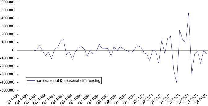
Foreign tourist arrivals after taking seasonal and non-seasonal differences.
4.1.1.2. Model identification
The autocorrelation (ACF) and partial autocorrelation functions (PACF) estimated from the tourist data reveal a strong seasonal pattern. The PACF has prominent spikes at lags (2, 4, and 8), which suggest seasonal and non-seasonal autoregressive processes. The ACF and PACF functions from both seasonal and non-seasonal differenced series suggest three tentative SARIMA Intervention models (2,1,0)(2,1,0)4, (1,1,0)(2,1,0)4, and (2,1,0)(1,1,0)4. Both the Akaike information criterion (AIC) (Akaike, 1974) and Schwarz Bayesian criterion (SBC) (Schwarz, 1978) are employed to select the best SARIMA Intervention model. Being loss functions, the model with the smallest value for AIC and SBC is selected as the best model. The SARIMA Intervention model (2,1,0)(2,1,0)4 had the lowest AIC and SBC values, therefore it is deemed the best SARIMA model (Table 3 ).
Table 3.
Estimation results of SARIMA Intervention and Trend models
| Variables | SARIMA Intervention |
Trend model |
||||
|---|---|---|---|---|---|---|
| Coefficients | SD | t | Coefficients | SD | t | |
| AR(1) | −0.44** | 0.13 | −3.44 | |||
| AR(2) | −0.47** | 0.13 | −3.65 | |||
| SAR(1) | −0.87** | 0.12 | −7.06 | |||
| SAR(2) | −0.46** | 0.14 | −3.34 | |||
| T | 4279.27* | 2073.47 | 2.06 | |||
| t2 | 132.44** | 29.30 | 4.52 | |||
| Constant | 743,032.62 | 28,190.81 | 26.36 | |||
| IMF | 83,484.05* | 39,407.63 | 2.12 | 84,242.84** | 26,076.07 | 3.23 |
| Terrorism | −98,226.66* | 49,112.48 | −2.00 | −65,168.65** | 18,116.21 | −3.60 |
| World Cup | 134,242.33* | 50,890.75 | 2.64 | 119,155.64** | 18,637.18 | 6.39 |
| SARS | −292,077.61** | 49,054.47 | −5.95 | −295,328.68* | 141,615.70 | −2.09 |
SARIMA Intervention (2,1,0)(2,1,0)4 : AIC=1497, SBC=1514; SARIMA Intervention (1,1,0)(2,1,0)4 : AIC=1507, SBC=1522; SARIMA Intervention (2,1,0)(1,1,0)4: AIC=1503, SBC=1520; F=106.19(df=6), p<0.001, R2=0.92.
p<0.05.
p<0.01.
4.1.1.3. Estimation results
As shown in Table 3, in the SARIMA (2,1,0)(2,1,0)4 model, the seasonal and non-seasonal terms are statistically significant at p<0.01 All interventions variables are statistically significant at p<0.05 and have the expected signs. IMF (Asian Financial) Crisis and World Cup coefficients are positive, whereas terrorism and SARS are negative. Estimations were performed using SPSS Statistical Program (version 12.0).
The residual ACF of the SARIMA (2,1,0)(2,1,0)4 Intervention model has no spikes at all lags (Fig. 3 ). Further, the Box–Ljung Q-statistics (Box & Pierce, 1970) are not statistically significant at every lag indicating that the probability that the residual autocorrelations are not white noise is less than 5% (Dharmaratne, 1995). The SARIMA model has accurate within sample forecasts (Fig. 4 ) with a MAPE of 4.5%. Given the model satisfies the above diagnostic criteria and provides accurate forecasts, we conclude that the SARIMA (2,1,0)(2,1,0)4 Intervention model is appropriate. Using a recursive forecasting approach, the SARIMA Intervention model forecasted approximately 2 million potential foreign visitors for the 3rd quarter of 2012, the quarter the Expo is to be held (Table 4 ).
Fig. 3.

ACF and Box–Ljung Q-statistics for the model residuals.
Fig. 4.

Forecasts of quarterly foreign tourist arrivals by the SARIMA Intervention, Trend, and Winters models.
Table 4.
Foreign tourist demand for the Expo based on the three quantitative models
| Model | Forecasts for Expo perioda |
WTVb (%) |
Mean demand |
MAPEc (%) |
|---|---|---|---|---|
| A | B | A×B | ||
| SARIMA1 | 2,001,652 | 28.2 | 564,466 | 4.5 |
| Winters2 | 1,921,733 | 28.2 | 541,929 | 5.0 |
| Trend3 | 2,229,182 | 28.2 | 628,629 | 5.5 |
Taking forecasts for the 3rd quarter of 2012, the quarter the Expo is to be held.
Willingness-to-visit (WTV) the Expo, percentage of tourist indicating they were either likely to visit or very likely to visit based on the foreign tourist survey.
0%⩽MAPE<10%: very accurate forecasts (Lewis, 1982).
4.1.2. Winters model
The sum of squared errors is minimized in the Winters model when the parameters are α=0.5, β=0.0, and γ=0.0. A value of 0.5 for the parameter α indicates that the current single smoothed values were predicted based on the moderate weight on both current values adjusted by seasonality and previous smoothed and trend values. The parameter β=0.0 implies that the current trend values are a function of the previous trend values without considering the difference in the smoothed values. Finally, the parameter γ=0.0 indicates the current seasonal component is a function of the previous seasonal component without considering the current values to be adjusted by the smoothed values. Similar to the SARIMA model, the Winters model has accurate within sample forecasts (Fig. 4) with a MAPE of 5.0%. The Winters model predicted approximately 1.9 million foreign tourists for the 3rd quarter of 2012 (Table 4). Estimations were performed using SPSS Statistical Program (version 12.0).
4.1.3. Trend model
The White Heteroskedasticity test indicates that heteroskedasticity existed (F=7.65, p<0.001) in the trend model. Therefore, robust regression (Huber–White sandwich estimators) using STATA 9.0 (Hamilton, 2003) is employed. As shown in Table 3, the trend model is statistically significant (F=106.19, p<0.001, R 2=0.92). All trend and intervention variables are significant at p<0.05 or less. The intervention variables have the expected signs in that IMF (Asian Financial) Crisis and World Cup coefficients are positive, whereas, terrorism and SARS coefficients are negative. As with the other models, the trend model provides accurate within sample forecasts (MAPE=5.5%) (Fig. 4). The trend model forecasted approximately 2.2 million foreign tourists for the 3rd quarter of 2012 (Table 4).
In summary, using MAPE as the measure of accuracy indicates that all three models performed well, based on values of MAPE being less than 10% (Goh & Law, 2002; Lewis, 1982). The SARIMA Intervention model performed slightly better with the lowest MAPE of 4.5%, followed by Winters model (MAPE=5.0%), and robust trend model (MAPE=5.5%). As shown in Table 4, forecasts by SARIMA Intervention model (2 million) were found similar to those by Winters model (1.9 million), but the trend model predicted a slightly larger tourism demand (2.2 million).
4.1.4. Forecasts of Expo demand by foreign tourists
Approximately twenty-eight percent (28.2%) of the foreign tourist surveyed indicated they were likely to visit (4 on the Likert-type scale) or very likely to visit (5 on the Likert scale). The percentage of tourist responding as a 4 or a 5 is assumed to be the WTV the Expo based on the previous work by Lee (2003). The number of foreign visitors to the Expo is then estimated by multiplying the tourist forecasts for the Expo period by WTV. Expo demand by foreign tourists is forecasted to be between 541,929 and 628,629 visitors (Table 4) by the three models. In this study, Expo demand predicted by the SARIMA Intervention model of 564,466 foreign visitors is chosen as our “best guess” because it provides a middle of the road forecast and the SARIMA Intervention model has the smallest MAPE.
4.2. The Expo demand for domestic visitors
4.2.1. Demand by domestic adult visitors
Expo demand by the domestic adult population in the year of 2012 is presented in Table 5 by region. WTV for the Yeosu Expo is calculated based on the results of national on-site survey in 16 regions. As in the foreign estimations, it is assumed the WTV percentage is represented by the percentage of respondents indicating a 4 (likely to visit) and a 5 (very likely to visit) on the Likert-type scale. WTV ranged from the low of 10.7% for Ulsan to the high of 41.6% for Jeonnam province. Survey results indicate the regions closer to the venue of the Expo generally have higher WTV. For example, Jeonnam, Kwangju, and Jeonbuk provinces, which are close to the Yeosu, have relatively large WTV, 41.6%, 38.9%, and 34.9%. On the other hand, Jeju, Kangwon, Kyongbuk, and Ulsan provinces which are further away from the venue have smaller WTV, ranging from 10.7% to 13.4%. This finding implies that distance between origin and destination is likely to act as a deterrent to attending the Expo. Expo demand by domestic adults is predicted by multiplying adult population in 2012 by WTV for each region and then summing the regional demands. Approximately 6.7 million domestic adults are predicted to attend the Expo (Table 5). Although Seoul metropolitan city and Kyonggi province have low WTV, predicted demands from these regions are relatively larger than less populated regions with larger WTV, because the these two regions have the largest populations in Korea.
Table 5.
Forecasts of the Expo demand for domestic adult by 16 regions
| Region | Adult population (2012) |
WTVa (%) |
Total demand |
|---|---|---|---|
| A | B | A×B | |
| Seoul | 7,363,660 | 20.2 | 1,487,459 |
| Busan | 2,562,995 | 19.9 | 510,036 |
| Daegu | 1,774,777 | 20.3 | 360,280 |
| Inchon | 1,899,237 | 14.9 | 282,986 |
| Kwangju | 989,043 | 38.9 | 384,738 |
| Daejon | 1,079,132 | 18.7 | 201,798 |
| Ulsan | 815,184 | 10.7 | 87,225 |
| Kyonggi | 8,572,496 | 14.6 | 1,251,584 |
| Kangwon | 966,481 | 12.0 | 115,978 |
| Chungbuk | 995,581 | 16.0 | 159,293 |
| Chungnam | 1,342,216 | 18.0 | 241,599 |
| Jeonbuk | 1,086,019 | 34.9 | 379,021 |
| Jeonnam | 1,060,007 | 41.6 | 440,963 |
| Kyongbuk | 1,681,392 | 13.4 | 225,307 |
| Kyongnam | 2,107,846 | 23.9 | 503,775 |
| Jeju | 365,132 | 11.5 | 41,990 |
| Total | 34,661,198 | 6,674,031 |
Willingness-to-visit (WTV) the Expo, percentage people indicating they were either likely to visit or very likely to visit based on the national survey. The WTV was based on the question including the admission fee (US$ 21) in order to provide a conservative estimate of the number of visitors.
4.2.2. Demand by domestic adolescents
Approximately 1.7 million adolescents are predicted to visit the Expo (Table 6 ). The regional demand patterns displayed by adult visitors are also shown in the number of adolescent visitors. In spite of relatively low WTV, Seoul metropolitan city and Kyonggi province are predicted to provide the largest number of visitors because of their large population bases, whereas, Ulsan and Jeju have the smallest demand for the Expo.
Table 6.
Forecasts of Expo demand for domestic adolescents by 16 regions
| Region | Adult population (2012) |
Percent of population age 30–49a (%) |
WTVb (%) |
Adolescent per parentc |
Adolescent population (2012) |
Total demand |
|---|---|---|---|---|---|---|
| A | B | C | D=E/(A×B) | E | A×B×C×D | |
| Seoul | 7,363,660 | 48.8 | 20.2 | 0.44 | 1,574,170 | 317,982 |
| Busan | 2,562,995 | 43.3 | 19.9 | 0.49 | 539,095 | 107,280 |
| Deagu | 1,774,777 | 47.0 | 20.3 | 0.55 | 455,994 | 92,567 |
| Inchon | 1,899,237 | 48.3 | 14.9 | 0.52 | 476,378 | 70,980 |
| Kwangju | 989,043 | 49.0 | 38.9 | 0.63 | 306,964 | 119,409 |
| Daejon | 1,079,132 | 48.8 | 18.7 | 0.53 | 281,386 | 52,619 |
| Ulsan | 815,184 | 49.0 | 10.7 | 0.54 | 215,515 | 23,060 |
| Kyonggi | 8,572,496 | 51.4 | 14.6 | 0.52 | 2,285,556 | 333,691 |
| Kangwon | 966,481 | 43.6 | 12.0 | 0.58 | 244,418 | 29,330 |
| Chungbuk | 995,581 | 46.4 | 16.0 | 0.58 | 266,327 | 42,612 |
| Chungnam | 1,342,216 | 45.1 | 18.0 | 0.58 | 351,405 | 63,253 |
| Jeonbuk | 1,086,019 | 42.4 | 34.9 | 0.66 | 304,036 | 106,109 |
| Jeonnam | 1,060,007 | 40.7 | 41.6 | 0.65 | 282,031 | 117,325 |
| Kyongbuk | 1,681,392 | 43.2 | 13.4 | 0.54 | 393,865 | 52,778 |
| Kyongnam | 2,107,846 | 46.6 | 23.9 | 0.58 | 565,534 | 135,163 |
| Jeju | 365,132 | 48.0 | 11.5 | 0.63 | 110,226 | 12,676 |
| Total | 34,661,198 | 8,652,900 | 1,676,834 |
Parent groups with ages 30–49 who are more likely to have adolescent in the household according to Korea National Statistical Office (2006b). Thus, proportion of parents accompanying adolescent was computed by dividing population of ages 30–49 by all adult population.
Willingness-to-visit (WTV) the Expo, percentage people indicating they were either likely to visit or very likely to visit based on the national survey (see Table 5).
Adolescents to be accompanied by parent, dividing adolescent population by population age 30–49.
4.3. Total demand
Total demand for the Expo is predicted to be approximately 8.9 million visitors. Of these 8.9 million visitors, domestic adults are the largest category with 6.7 million visitors, followed by domestic adolescents (1.7 million), and foreign tourists (0.5 million). Unfortunately, the Korea National Statistical Office does not provide standard errors or confidence intervals with their population estimates. This limitation forces only point estimates for the domestic demand for the Expo to be generated. Given the magnitude of domestic demand relative to foreign demand, confidence intervals for total Expo demand would be meaningless based only on the quantitative model.
4.4. Qualitative forecasts by the Delphi method
Twenty-seven of the 29 panel members responded to both the first and second rounds of the Delphi survey, representing a 93.1% of response rate (Table 7 ). The mean and median varied little between the two rounds changing by 0.3% and 1.4%, whereas, the mode decreased by 12.5%. In round two, these statistics in magnitudes vary by approximately 3%. Standard deviations of forecasted demand decreased from 1,240,500 in the 1st round to 887,300 in the 2nd round. Skewness and kurtosis decreased for 2nd round as compared to 1st round. In addition, the lowest forecast increased from 4 million in the 1st round to 5 million in the 2nd round, whereas the highest forecast decreased from 9 million in the 1st round to 8.5 million in the 2nd round. Taking all statistics into account, it appears that convergence in forecasts by the experts has occurred between two rounds of the Delphi survey.
Table 7.
Results of the Delphi method for demand for Yeosu Expo (number of visitors)
| Statistics | 1st round | 2nd round |
|---|---|---|
| Mean | 6,795,200 | 6,774,100 |
| Median | 7,000,000 | 6,900,000 |
| Mode | 8,000,000 | 7,000,000 |
| Range | ||
| Low | 4,000,000 | 5,000,000 |
| High | 9,000,000 | 8,500,000 |
| Standard deviation | 1,240,500 | 887,300 |
| 95% confidence interval | ||
| Lower bound | 6,304,500 | 6,423,100 |
| Upper bound | 7,285,901 | 7,125,100 |
| Skewness | −0.553 | −0.042 |
| Kurtosis | −0.410 | 0.252 |
| No. of responses | 27 | 27 |
| No. of experts | 29 | 29 |
Given the mean, median, and mode values are similar, the mean value is used as the forecasts by the panel members. Based on the mean value, panel members predicted 6.8 million foreign and domestic visitors to the Expo. The 95% confidence interval ranges from a lower bound of 6.4 million to an upper bound of 7.1 million visitors. Comments by some of the experts indicated that the distance from major metropolitan cities to the Expo site would act as a major barrier to discourage people to visit the Expo. On the other hand, a few experts stated that the Expo event would act as an attraction to encourage people to visit Yeosu.
5. Conclusions and discussions
While forecasting tourism demand usually involves the use of quantitative techniques, predicting the demand for unprecedented events such as an international tourism Expo presents challenges because of the lack of appropriate historical data. To overcome this challenge, this study combined quantitative techniques with WTV generated from survey data to predict the demand for the Yeosu Expo. The combined technique involved: forecasting foreign tourist arrivals using quantitative forecasting models, projected populations, and estimating WTV the Expo using a national survey and a survey of foreign tourists.
Empirical results of quantitative forecasting models of foreign tourists indicate that all three time-series models used in this study performed well in terms of MAPE. All MAPE's are less than 10%. The SARIMA Intervention model slightly outperformed the Winters model and the trend model in within sample forecasting. Using a middle of road estimate, a half million foreign tourists are expected to visit the Expo.
WTV obtained from the national survey indicates that the closer a region is to the Expo site, the larger the WTV to the site. The distance between origin and destination has been discussed in gravity models as deterrent factor to traveling (Cesario, 1973; Reece, 2001; Vanhove, 1980; Var & Lee, 1993). The WTV results support this finding from the gravity models. This study did not attempt to forecast domestic populations, but rather used existing population forecasts from the Korea National Statistical Office. Breaking down the forecast for the Expo by adult and adolescent visitor gives an estimate of 6.7 million adult visitors and 1.7 million adolescent visitors. Total visitors are forecasted at approximately 8.9 million people including 0.5 million foreign tourists.
As a comparison to the above methodology, the above estimates are compared to estimates obtained using the Delphi method. Based on the Delphi survey, 27 experts predicted approximately 6.8 million visitors to the Expo. Comments made by panel members, indicated they considered distance or accessibility as the most important barrier to increasing Expo demand. Experts in the Delphi method predicted lower demand for the Expo than the combined quantitative techniques with WTV surveys. Both methods have merit and only time will tell which estimates are closest.
It is interesting to compare the above forecasts with other forecasts of the demand for the Expo. An official of the Bureau International des Expositions (BIE) expected the Expo demand between 7 and 9 million visitors, a former BIE official predicted 8 million, and the Director of Producer of the 2006 Aichi Expo predicted 7–8 million (Korea Marine Institute, 2006). The lower boundary predicted by overseas experts is similar to forecasts by local experts, whereas the upper boundary predicted by overseas experts is to be similar to forecasts by the quantitative techniques with WTV surveys. Another interesting comparison is to compare the estimates of the Yeosu Expo to the number of visitors to previous Expos. The 93 Daejon Expo, was the first BIE Expo held in South Korea. The number of visitors to the Daejon Expo was 14 million people over 3 months (Korea Marine Institute, 2006). Twenty-two million people attended the 2005 Aichi Expo in Japan over 6 months, which is 7 million more visitors than the sponsors expected to attend (Aichi Expo Organizing Committee, 2006). The number of visitors to both of these previous Expos is higher than even the most optimistic demand forecast for the Yeosu Expo. One potential reason is both the Daejon Expo and the Aichi Expo were held in areas that have relatively larger population bases than the Yeosu area. Another reason is there are two types of Expos, one held for 3 months and the other for 6 months. The Aichi Expo lasted 6 months as compared to 3 months planned for the Yeosu Expo. These comparisons between past Expos and forecasted demand, along with experts’ opinions further suggest that distance and capacities of hosting city are significant factors determining demand for Expos.
From a practical standpoint, results from forecasting the Expo demand are useful for the planners and policy-makers. First, forecasts of the Expo demand are important in the bidding process of the international tourism Expo. One selection criteria of the host city is the magnitude of demand, as well as the appropriateness of the forecasting methods used. Second, forecasts of Expo demand may not only help generate public support, but are also important to help avoid shortages or surpluses in the tourism businesses (Burger et al., 2001). The forecasts of the Expo demand provide managers with planning infrastructure, such as magnitude of Expo site and facilities, number of hotel rooms, expansion of road and transportation system, etc. These infrastructures are highly dependent upon estimates of tourism demand because they require huge financial investment from private and public sectors.
Edgell and Seely (1980) insist that tourism is based on both demand- and supply-side in the managerial and practical points of view. The forecasted demand of between 6.8 and 8.9 million visitors will not be realized unless the capacity of accommodations, road and transportation system, and Expo site can meet this demand. An engineering company which is responsible for the site planning for the Expo unofficially predicted that the Expo site is able to accommodate approximately 8 million visitors in terms of the capacity of site and road system. The higher estimates of Expo demand predicted by quantitative approaches with WTV appeared to slightly exceed the supply-side, whereas the smaller estimates of Expo demand predicted by the Delphi method is within the supply-side capabilities.
Two challenging areas in tourism forecasting are how to obtain better WTV from surveys and how well the estimated WTV reflect actual visits. One beneficial avenue for future research is to develop reliable indices of actualization which will contribute to improving the forecasting accuracy and providing benefit to event managers in the planning stage.
Contributor Information
Choong-Ki Lee, Email: cklee@khu.ac.kr.
Hak-Jun Song, Email: bloodia00@hotmail.com.
James W. Mjelde, Email: j-mjelde@tamu.edu.
References
- Akaike H. A new look at the statistical model identification. IEEE Transactions on Automatic Control. 1974;19(6):716–723. [Google Scholar]
- Aichi Expo Organizing Committee (2006). Visitors statistics. Available from 〈http://www.expo2005.or.jp〉.
- Archer B.H. University of Wales Press; Bangor, UK: 1976. Demand forecasting in tourism. [Google Scholar]
- Archer B.H. Demand forecasting and estimation. In: Ritchie J.R.B., Goeldner C.R., editors. Travel, tourism, and hospitality research. Wiley; New York: 1987. pp. 77–85. [Google Scholar]
- Artus J.E. An econometric analysis of international travel. IMF Staff Paper. 1972;19(3):579–614. [Google Scholar]
- Ascher W. Johns Hopkins University Press; Baltimore: 1978. Forecasting: An appraisal policy-makers and planners. [Google Scholar]
- Barry K., O’Hagan J. An econometric study of British tourist expenditure in Ireland. Economic and Social Review. 1972;3(2):143–161. [Google Scholar]
- Box G.E.P., Pierce D.A. Distribution of residual autocorrelations in autoregressive integrated moving average time series models. Journal of the American Statistical Association. 1970;65(332):1509–1526. [Google Scholar]
- Box G.E.P., Tiao G.C. Intervention analysis with applications to economic and environmental problems. Journal of the American Statistical Association. 1975;70(349):70–79. [Google Scholar]
- Burger C.J.S.C., Dohnal M., Kathrada M., Law R. A practitioners guide to time-series methods for tourism demand forecasting—a case study of Durban, South Africa. Tourism Management. 2001;22(4):403–409. [Google Scholar]
- Calantone R.J., Di Benedetto A., Bojanic D. A comprehensive review of the tourism forecasting literature. Journal of Travel Research. 1987;26(2):28–39. [Google Scholar]
- Cesario F.J. A generalized trip distribution model. Journal of Regional Science. 1973;13(2):233–247. [Google Scholar]
- Cho V. A comparison of three different approaches to tourist arrival forecasting. Tourism Management. 2003;24(3):323–330. [Google Scholar]
- Crouch G.I. Effect of income and price on international tourism. Annals of Tourism Research. 1992;19(4):643–664. [Google Scholar]
- Crouch G.I. The study of international tourism demand: A review of findings. Journal of Travel Research. 1994;33(1):12–23. [Google Scholar]
- Chu F.L. Forecasting tourism: A combined approach. Tourism Management. 1998;19(6):515–520. [Google Scholar]
- Dalkey N., Helmer O. An experimental application of the Delphi method to the use of experts. Management Science. 1963;9(3):456–467. [Google Scholar]
- Dharmaratne G.S. Forecasting tourist arrivals in Barbados. Annals of Tourism Research. 1995;22(4):804–818. [Google Scholar]
- Dickey D.A., Fuller W.A. Distribution of the estimators for autoregressive time series with a unit root. Journal of the American Statistical Association. 1979;74(366):427–431. [Google Scholar]
- Dickey D.A., Hasza D.P., Fuller W.A. Testing for unit roots in seasonal time series. Journal of the American Statistical Association. 1984;79(386):355–367. [Google Scholar]
- Di Matteo L., Di Matteo R. The determinants of expenditures by Canadian visitors to the United States. Journal of Travel Research. 1993;31(4):34–42. [Google Scholar]
- Enders W. 1st ed. Wiley; New York: 1995. Applied econometric time series. [Google Scholar]
- Edgell D., Seely R. A multi-stage model for the development of international tourism forecasts for states and regions. In: Hawkins D.E., Shafer E.L., Rovelstad J.M., editors. Tourism planning and development issues. George Washington University; Washington, DC: 1980. pp. 407–410. [Google Scholar]
- Gerakis A.S. Effects of exchange-rate devaluation and revaluations on receipts from tourism. IMF Staff Paper. 1965;12(2):365–384. [Google Scholar]
- Getz D. Van Nostrand Reinhold; New York: 1991. Festivals, special events, and tourism. [Google Scholar]
- Geurts M.D., Ibrahim I.B. Comparing the Box–Jenkins approach with the exponentially smoothed forecasting model application to Hawaii tourists. Journal of Marketing Research. 1975;12(2):182–188. [Google Scholar]
- Geurts M.D., Ibrahim I.B. Forecasting the Hawaiian tourist market. Journal of Travel Research. 1982;21(1):18–21. [Google Scholar]
- Goh C., Law R. Modeling and forecasting tourism demand for arrivals with stochastic nonstationary seasonality and intervention. Tourism Management. 2002;23(5):499–510. [Google Scholar]
- Glass G.V. Estimating the effects of intervention into a nonstationary time series. American Educational Research Journal. 1972;9(3):463–477. [Google Scholar]
- Gray H.P. The demand for international travel by the United States and Canada. International Economic Review. 1966;7(1):83–92. [Google Scholar]
- Green B., Chalip L. Sport tourism as the celebration of subculture. Annals of Tourism Research. 1998;25(2):275–291. [Google Scholar]
- Hamilton L.C. Duxbury; California: 2003. Statistics with STATA (version 9) [Google Scholar]
- Han Z., Durbarry R., Sinclair M.T. Modelling US tourism demand for European destinations. Tourism Management. 2006;27(1):1–10. [Google Scholar]
- Jud G.D., Joseph H. International demand for Latin American tourism. Growth and Change. 1974;5(1):25–31. [Google Scholar]
- Kaynak E., Macaulay J.A. The Delphi technique in the measurement of tourism market potential. Tourism Management. 1984;5(2):87–101. [Google Scholar]
- Kim J.H., Moosa I.A. Forecasting international tourist flows to Australia: A comparison between the direct and indirect methods. Tourism Management. 2005;26(1):69–78. [Google Scholar]
- Korea Marine Institute. (2006). Demand for the Yeosu Expo: Internal report. Seoul: Korea Marine Institute.
- Korea National Statistical Office. (2005). National population. Available from 〈http://www.nso.go.kr〉.
- Korea National Statistical Office. (2006a). Projection of population. Available from 〈http://www.nso.go.kr〉.
- Korea National Statistical Office. (2006b). Statistics on berth and death. Available from 〈http://www.nso.go.kr〉.
- Korean National Tourism Organization. (2006). Tourism Statistics. Available from 〈http://www.knto.or.kr〉.
- Kulendran N., Witt S.F. Forecasting the demand for international business tourism. Journal of Travel Research. 2003;41(3):265–271. [Google Scholar]
- Kulendran N., Witt S.F. Leading indicator tourism forecasts. Tourism Management. 2003;24(5):503–510. [Google Scholar]
- Laber G. Determinants of international travel between Canada and the United States. Geographical Analysis. 1969;1(4):329–336. [Google Scholar]
- Lee C.K. Major determinants of international tourism demand for South Korea: Inclusion of marketing variable. Journal of Travel and Tourism Marketing. 1996;5(1/2):101–118. [Google Scholar]
- Lee C.K. Ilshinsa; Seoul: 2003. Applied economics of tourism (Korean version) [Google Scholar]
- Lee C.K., Kim J.H. International tourism demand for the 2002 World Cup Korea: A combined forecasting technique. Pacific Tourism Review. 1998;2(2):1–10. [Google Scholar]
- Lee C.K., Lee Y.K., Lee B.K. Korea's destination image formed by the 2002 World Cup. Annals of Tourism Research. 2005;32(4):839–858. [Google Scholar]
- Lee C.K., Lee Y.K., Wicks B. Segmentation of festival motivation by nationality and satisfaction. Tourism Management. 2004;25(1):61–70. [Google Scholar]
- Lee C.K., Taylor T. Critical reflections on the economic impact assessment of a mega-event: the case of 2002 FIFA World Cup. Tourism Management. 2005;26(4):595–603. [Google Scholar]
- Lee C.K., Var T., Blaine T.W. Determinants of inbound tourist expenditures. Annals of Tourism Research. 1996;23(3):527–542. [Google Scholar]
- Lewis C.D. Butterworth; London: 1982. Industrial and business forecasting methods. [Google Scholar]
- Li G., Song H., Witt S.F. Recent developments in econometric modeling and forecasting. Journal of Travel Research. 2005;44(1):83–99. [Google Scholar]
- Li G., Wong K.F., Song H., Witt S.F. Tourism demand forecasting: A time varying parameter error correction model. Journal of Travel Research. 2006;45(2):175–185. [Google Scholar]
- Lim C. Review of international tourism demand models. Annals of Tourism Research. 1997;24(4):835–849. [Google Scholar]
- Lim C. A meta-analytic review of international tourism demand. Journal of Travel Research. 1999;37(3):273–284. [Google Scholar]
- Lim C. Time series forecasts of international travel demand for Australia. Tourism Management. 2002;23(4):389–396. [Google Scholar]
- Lim C., McAleer M. Forecasting tourist arrivals. Annals of Tourism Research. 2001;28(4):965–977. [Google Scholar]
- Lim C., McAleer M. Time series forecasts of international travel demand for Australia. Tourism Management. 2002;23(4):389–396. [Google Scholar]
- Liu J.C. Hawaii tourism to the year 2000: A Delphi forecast. Tourism Management. 1988;9(4):279–290. [Google Scholar]
- Loeb P.D. International travel to the United States: An econometric evaluation. Annals of Tourism Research. 1982;9(1):7–20. [Google Scholar]
- Nelson J.P. Consumer bankruptcies and the Bankruptcy Reform Act: A time-series intervention analysis, 1960–1997. Journal of Financial Services Research. 2000;17(2):181–200. [Google Scholar]
- Makridakis S. The art and science of forecasting: An assessment and future directions. International Journal of Forecasting. 1986;2(1):15–39. [Google Scholar]
- Makridakis S., Wheelwright S.C. Wiley; New York: 1978. Forecasting: Methods and applications. [Google Scholar]
- Makridakis S., Wheelwright S.C., Hyndman R.J. 3rd ed. Wiley; New York: 1998. Forecasting: Methods and applications. [Google Scholar]
- Makridakis S., Wheelwright S.C., Victor E. 2nd ed. Wiley; New York: 1983. Forecasting: Methods and applications. [Google Scholar]
- Martin C.A., Witt S.F. Accuracy of econometric forecasts of tourism. Annals of Tourism Research. 1989;16(3):407–428. [Google Scholar]
- Prideaux B., Laws E., Faulkner B. Events in Indonesia: Exploring the limits to formal tourism trends forecasting methods in complex crisis situations. Tourism Management. 2003;24(4):475–487. [Google Scholar]
- Quayson J., Var T. A tourism demand function for the Okanagan, BC. Tourism Management. 1982;3(2):108–115. [Google Scholar]
- Reece W.S. Travelers to Las Vegas and to Atlantic City. Journal of Travel Research. 2001;39(3):275–284. [Google Scholar]
- Sheldon P.J. Forecasting tourism: Expenditures versus arrivals. Journal of Travel Research. 1993;32(1):13–20. [Google Scholar]
- Song H., Witt S.F. Forecasting international tourist flows to Macau. Tourism Management. 2006;27(2):214–224. [Google Scholar]
- Stronge W.B., Redman M. US tourism in Mexico: An empirical analysis. Annals of Tourism Research. 1982;9(1):21–35. [Google Scholar]
- Schwarz G. Estimating the dimension of a model. Annuals of Statistics. 1978;6(2):461–464. [Google Scholar]
- Uysal M., Cromption J.L. Determinants of demand for international tourist flows to Turkey. Tourism Management. 1984;5(4):288–297. [Google Scholar]
- Uysal M., Cromption J.L. An overview of approaches used to forecast tourism demand. Journal of Travel Research. 1985;23(4):7–15. [Google Scholar]
- Van Doorn J.W.M. Tourism forecasting and the policy maker. Tourism Management. 1984;5(1):24–39. [Google Scholar]
- Vanhove N. Forecasting in tourism. Revue de Tourisme. 1980;35(3):2–7. [Google Scholar]
- Var T., Lee C.K. Tourism forecasting: State-of-the-art techniques. In: Khan M.A., Olsen M.D., Var T., editors. VNR's encyclopedia of hospitality and tourism. Van Nostrand Reinhold; New York: 1993. pp. 679–696. [Google Scholar]
- Wheelwright S.C., Makridakis S. 4th ed. Wiley; New York: 1985. Forecasting methods for management. [Google Scholar]
- WHO . World Health Organization; Geneva: 2003. Severe acute respiratory syndrome (SARS): Status of the outbreak and lessons for the immediate future. [Google Scholar]
- Witt C.A., Witt S.F. Appraising an econometric forecasting model. Journal of Travel Research. 1990;28(3):30–34. [Google Scholar]
- Witt S.F., Martin C.A. Econometric models for forecasting international tourism demand. Journal of Travel Research. 1987;25(3):23–30. [Google Scholar]
- Wong K.F., Song H., Chon K.S. Bayesian models for tourism demand forecasting. Tourism Management. 2006;27(5):773–780. [Google Scholar]