DeepCut: Object Segmentation from Bounding Box Annotations using Convolutional Neural Networks

Abstract

In this paper, we propose DeepCut, a method to obtain pixelwise object segmentations given an image dataset labelled weak annotations, in our case bounding boxes. It extends the approach of the well-known GrabCut [1] method to include machine learning by training a neural network classifier from bounding box annotations. We formulate the problem as an energy minimisation problem over a densely-connected conditional random field and iteratively update the training targets to obtain pixelwise object segmentations. Additionally, we propose variants of the DeepCut method and compare those to a naïve approach to CNN training under weak supervision. We test its applicability to solve brain and lung segmentation problems on a challenging fetal magnetic resonance dataset and obtain encouraging results in terms of accuracy.

I. Introduction

Many modern medical image analysis methods that are based on machine learning rely on large amounts of annotations to properly cover the variability in the data (e.g. due to pose, presence of a pathology, etc). However, the effort for a single rater to annotate a large training set is often not feasible. To address this problem, recent studies employ forms of weak annotations (e.g. image-level tags, bounding boxes or scribbles) to reduce the annotation effort and aim to obtain comparably accurate results as to under full supervision (i.e. using pixelwise annotations) [2], [3], [4].

User-provided bounding boxes are a simple and popular form of annotation and have been extensively used in the field of computer vision to initialise object segmentation methods [1], [5]. Bounding boxes have advantages over other forms of annotations (e.g. scribbles or brush strokes [6], [7], [8]), as they allow to spatially constrain the problem (i.e. ideally, the object is unique to the bounding box region and fully contained in it). In a practical sense, bounding boxes can be defined via two corner coordinates, allowing fast placement (approximately 15 times faster than pixelwise segmentations [9]) and lightweight storage of the information. Considering the required interaction effort and the amount of provided information, these properties qualify bounding boxes as preferred weak annotation for image analysis methods.

In segmentation studies [1], [5], [10], bounding boxes are employed as both initialisation and spatial constraints for the segmentation problem. The above approaches model the image appearance (i.e., colours or greyscale intensity) and impose smoothness constraints upon the segmentation results for each image. However, given an image database and corresponding annotations, we can assume that objects share common shape and appearance information, which can be learned (i.e., instead of direct image-by-image object segmentation, a common model can be learned for the all images in the database). This is particularly interesting for segmentation problems on medical images, where typically an entire cohort is to be analysed for a specific organ or region, exhibiting large class similarity in terms of shape and appearance.

In this paper, we propose combining a neural network model with an iterative graphical optimisation approach to recover pixelwise object segmentations from an image database with corresponding bounding box annotations. The idea builds on top of the popular GrabCut [1] method, where an intensity appearance model is iteratively fitted to a region and subsequently regularised to obtain a segmentation. Similarly to this, the proposed DeepCut method iteratively updates the training targets (i.e. the class associated with a voxel location, described by an image patch) learned by a convolutional neural network (CNN) model and employs a fully connected conditional random field (CRF) to regularise the segmentation. The approach is formulated in a generic form and thus can be readily applied to any object or image modality. We briefly review recent advancements in the following section to put this approach into the context of the current state-of-the-art and highlight our contributions.

A. Related work

Graphical energy minimisation techniques are popular methods for regularised image segmentation due to inherent optimality guarantees and computational efficiency [11], [12]. They have been extensively used in the optimisation of interactive [6], [13], [14], [8] and fully automated segmentation methods [15], [16], [17], [18].

An iterative optimisation of such energy functionals allows to address more complex problems, such as the pixelwise segmentation from bounding box annotations. The popular GrabCut method [1] iteratively updates parameters of a Gaussian mixture model (GMM) and optimises the resulting energy with a graph cut. Lempitsky et al. [5] extended this method by adding a topological prior to prevent excessive shrinking of the region and Cheng et al. [10] improved upon its performance by employing a fast fully connected Conditional-Random Field (CRF) [19]. Similar approaches include the time-implicit propagation of levelsets via continuous max-flow [20], [21], iterative graph cuts [22] and the use of the expectation-maximisation (EM) algorithm [23], [24], [2].

Similarly to the above mentioned segmentation approaches, learning-based methods have been recently investigated to exploit the advantages of weak annotations, primarily to reduce the effort of establishing training data. In contrast to learning under full supervision (i.e. using pixelwise annotations), weakly supervised methods aim to learn from image-level tags, partial labels, bounding boxes, etc. and infer pixelwise segmentations.

Recently, several multiple instance learning (MIL) techniques were investigated, particularly when images could potentially contain multiple objects. Cinbis et al. [25] proposed a multi-fold MIL method to obtain segmentations from image level tags. Vezhnevets and Buhmann [26] addressed the problem with a Texton Forest [27] framework, extending it to MIL. With the re-emerging of convolutional neural networks [28], [29], MIL methods have been proposed to exploit such methods [30], [31]. However MIL-based methods, even when including additional modules under weak supervision [31], have not been able to achieve comparable accuracy to fully supervised methods [2]. However, latest developments using CNN learning with weakly supervised data have shown remarkable improvements in accuracy. Schlegl et al. [4] parse clinical reports to associate findings and their locations with optical coherence tomography images and further obtain segmentations of the reported pathology. Dai et al. [3] iterative between updating region proposals in bounding boxes and model training. Papandreou et al. [2] formulate an Expectation-Maximization (EM) algorithm [23] to iteratively update the training targets. Both of the latter methods were able to achieve comparable accuracy to those under full supervision.

B. Contributions

In this paper, we build upon the ideas of GrabCut [1], a well-known object segmentation method employed on single images. We extend the basic idea with recent advances in CNN modelling and propose DeepCut, a method to recover semantic segmentations given a database of images with corresponding bounding boxes. For this purpose, we formulate an iterative energy minimisation problem defined over a densely connected conditional random field (CRF) [19] and use it to update the parameters of a CNN model. We compare the proposed method against a fully supervised (CNN_FS) and a naïve approach to weakly supervised segmentation (CNN_naïve), to obtain upper and lower accuracy bounds for a given segmentation problem. Further, we examine the effect of region initialisation on the proposed method by providing a presegmentation within the bounding box, (DC_PS)). Finally, we compare all methods in their segmentation accuracy using a highly heterogeneous and challenging dataset of fetal magnetic resonance images (MRI) and further evaluate the performance to GrabCut [1], as an external method to this framework.

II. Methods

Let us consider segmentation problems using energy functionals over graphs as described in [11]. We seek a labelling f for each pixel i, minimising

$$E(f)=\sum _i{\psi }_u\left(f_i\right)+\sum _{i<j}{\psi }_p(f_i,f_j),$$ (1)

where ψ_u(f_i) serves as unary data consistency term, measuring the fit of the label f at each pixel i, given the data. Additionally, the pairwise regularisation term ψ_p(f_i,f_j) penalises label differences for any two pixel locations i and j. Typically, pairwise regularisation terms have the form of

$${\psi }_p(f_i,f_j)\propto \text{exp}\left(-\frac{{(I_i-I_j)}^2}{2{\theta }_{\beta }}\right),$$ (2)

and enforce contrast-sensitive smoothness penalties between the intensity vectors I_i and I_j [6], [17]. We can minimise the energy in Eq. (1) using a densely-connected CRF [19], where we replace the pairwise term with

$${\psi }_p\left(f_i\right)=g(i,j)[f_i\ne f_j],$$ (3)

consisting of two penalty terms modelling appearance (4a) and smoothness (4b) between the locations p_i and p_j:

$$g(i,j)={\omega }_1\text{exp}\left(-\frac{{|p_i-p_j|}^2}{2{\theta }_{\alpha }^2}-\frac{{|I_i-I_j|}^2}{2{\theta }_{\beta }^2}\right)$$ (4a)

$$+{\omega }_2\text{exp}\left(-\frac{{|p_i-p_j|}^2}{2{\theta }_{\gamma }^2}\right).$$ (4b)

The relative contributions of the two penalties is weighted by the regularisation parameters ω ₁and ω ₂ and the degrees of spatial proximity and similarity are controlled by θ_α and θ_β respectively [19].

The unary potential is computed independently for each pixel i by a data model with the parameters Θ that produces a distribution y_i over the label assignment given an input image or patch x and is defined as the negative log-likelihood of this probability:

$${\psi }_u\left(f_i\right)=-\text{log}P\left(y_i|x,\mathrm{\Theta }\right).$$ (5)

In contrast to [1], where the unary term is computed from a GMM of the observed colour or intensity vector, we employ a CNN with the parameters Θ. We describe the network architecture in Section II-B in detail.

A. Segmentation by Iterative Energy Optimisation

The proposed DeepCut method can be seen as an iterative energy minimisation method similar to GrabCut [1]. There are two key stages to both algorithms, model estimation and label update. GrabCut uses a GMM to parametrise the colour distributions of the foreground and background. In the model estimation stage the parameters Θ for the GMM are computed based on the current label assignment f for each pixel i. At the label update stage the pixels are relabelled based on the new model. DeepCut replaces the GMM with a Neural Network model and the graph cut solver from [11] with [19] on a densely-connected graph. In contrast to [1], and rather than recomputing our model, we make use of transfer learning [32] and reinitialise the CNN with the parameters of the last iteration.

This two-step iterative method is similar to an EM algorithm, consisting of an E-step (label update) and M-step (model update). Papandreou et al. [2] describe such a method to iteratively update f, however only employ regularisation as in Eq. (1) as a post-processing step during testing.

B. Convolutional Neural Network Model

The CNN is a hierarchically structured feed-forward neural network comprising of least one convolutional layer [28], [29]. Additionally, max-pooling layers downsample the input information to learn object representations at different scales. Downstream of several convolutional and max-pool layers is typically a layer of densely-connected neurons, reducing the output to a desired number of classes [4]. our CNN is a typical feed-forward neural network model which consist of convolutional layers (feature extraction), max-pooling layers (shift/scale invariance) and dense layers (classification stage). The network architecture used in this study is depicted in Fig. 1.

Fig. 1.

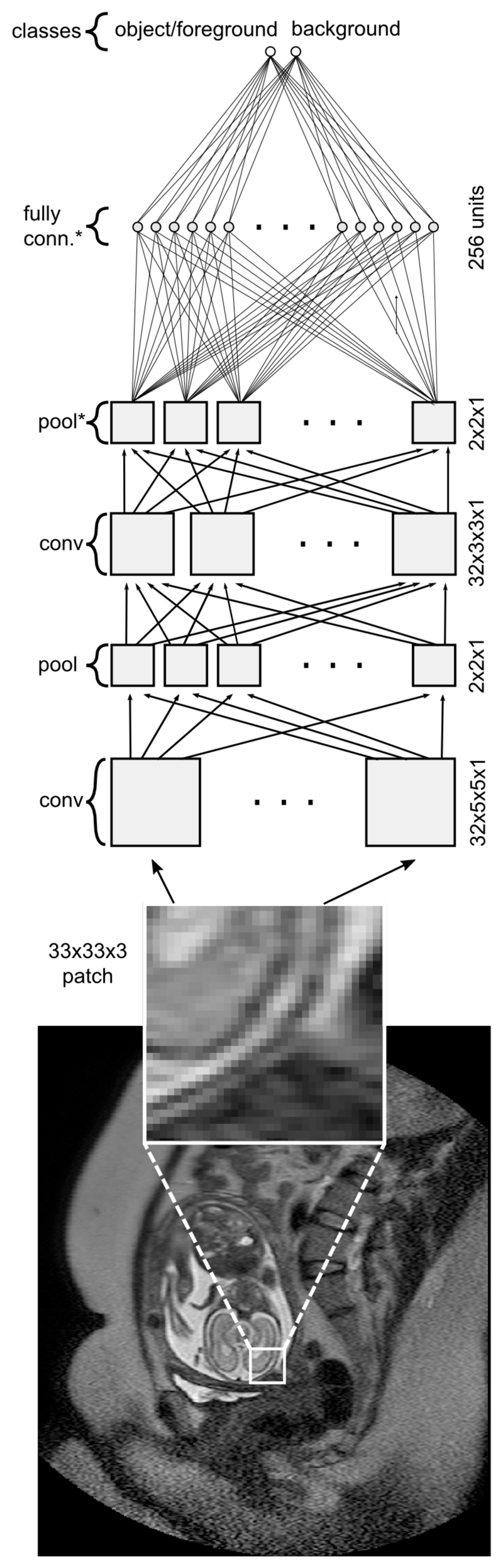
CNN architecture with convolutional (conv), max-pooling (pool) layers, and fully connected layers for foreground/background classification. Layer, which inputs are subjected to 50% dropout [33] are marked with *.

Input & Output Space

Given a database of size N containing images I = {I ₁,…,I_N} and corresponding bounding boxes B = {B ₁,…,B_N}, we attempt to learn pixelwise segmentations of the objects depicted in I and constrained to B. For this purpose, we employ a CNN with parameters Θ to classify image patches centred around a voxel location i into foreground and background.

We describe each voxel location i ∈ I_n as a 3D patch of size p_x × p_y × p_z, centred around X. Each patch X is associated with an integer value Y = {0,1}, representing background and foreground class of the centre voxel at i, respectively. The patch X serves as input to the network, which aims to predict Y. Because of anticipated motion artefacts between fetal MR slices, we decided to emphasise the in-plane context of our training patches, using a patch size of 33x33x3, rather than cubic patch dimensions.

Network Configuration

For the purpose of this study, we designed a simple CNN inspired by the well-known LeNet architecture [34]. While the proposed approach can employ other networks, we chose this configuration, as it is easily understandable and simple to reproduce. The CNN consists of two sets of convolutional (conv) and subsequent max-pooling (pool) layers. Since a convolution reduces the layer output by half the kernel size, we pad its output with zeros to preserve the size of the input tensor. The two serial conv/pool layers are attached to a layer with densely-connected (dense) neurons and an output layer with neurons associated with foreground and background. For regularisation purposes, we add dropout to both inputs of the dense and output layer, randomly sparsifying the signal and reducing the potential of over-fitting [33]. Figure 1 depicts the specific configuration, which has been fixed for all experiments in this study.

Training & Optimisation

In each epoch, we extract K = 10⁵ patches X_k from the training database, which are equally distributed between the classes Y_k. All CNN weights are initialised by sampling from a Gaussian distribution. We employ an adaptive gradient descent optimisation (ADAGRAD) [35] of mini-batches using a constant learning rate η = 0.015 for a fixed number of epochs. This has the advantage of adapting the learning rate locally for each feature, thus exhibiting more robust behaviour and faster convergence. The loss function is defined as the categorical cross-entropy between the true and coding distributions, respectively.

Data Augmentation

The training set undergoes data augmentation for better generalisation of the learned features and to prevent over-fitting to the training data. For this purpose, we add a Gaussian-distributed intensity offset to each patch with the standard deviation σ and randomly flip the patch across the spatial dimensions to increase the variation in the training data.

C. Naïve Learning Approach

If we assume that the patches describing the object constrained to the bounding box B are unique, we can attempt to classify patches X_i ∈ B into object and background, by using patches sampled from the bounding boxes as foreground targets. To obtain background targets, we can extend B to a halo region H, solely containing background voxels. A naïve approach to segmentation would be to assume that all X_i ∈ B belong to the object and all X_i ∈ H to the background. However, since the region B contains false positive locations (i.e., the object does not fully extend to the entire bounding box region, but is merely a subset of it), we will introduce errors into the model, which will impact the accuracy of the final segmentation. To ensure a fair comparison of the segmentation results, post-processing includes regularisation with a densely-connected CRF [19]. This naïve approach (CNN_naïve) is depicted in Figure 2.

Fig. 2.

Naïve CNN learning versus the proposed DeepCut approach, iteratively updating the learning target classes for input patches.

D. DeepCut

In order to develop a better approach compared to Section II-C, we start training the CNN model Θ with patches X sampled from B and H for foreground and background, respectively. In contrast to the naïve approach, we interrupt the training of Θ after a fixed number of epochs and update the classes Y for all voxels in B = R_FG ∪ R_BG, via inference and subsequent CRF regularisation, according to Section II-A. We continue training with the updated targets and reinitialise the CNN with Θ.

E. Region Initialisation

While methods such as DeepCut, GrabCut [1] or others [2], [3] rely on (approximately) globally optimal solvers (i.e., [11] and [19], respectively), the iterative nature of the algorithm will be limited to finding local optima. Thus the resulting segmentation is dependent on the initial regions R_FG and R_BG. Papandreou et al. [2] propose performing a presegmentation within B to initialise R_FG and R_BG closer to the object and observed large improvements in accuracy of the final segmentation. Similar initialisation can be done with the proposed DeepCut method and will be examined in Section III. In our experiments, we distinguish the variants of DeepCut initialised with bounding boxes and pre-segmentations with DC_bb and DC_PS, respectively.

III. Experiments

A. Image Data

For all experiments, we used the database in [36], consisting of MR images of 55 fetal subjects. The images were acquired on 1.5T MR scanner using a T2-weighted ssFSE sequence (scanning parameters: TR 1000ms, TE 98ms, 4mm slice thickness, 0.4mm slice gap). Most of the images contain motion artefacts that are typical for such acquisitions. The imaged population consists of 30 healthy subjects and 25 subjects with intrauterine growth restriction (IUGR) and their gestational age ranged from 20 to 30 weeks. For all images, the brain and the lung regions have been manually segmented by an expert rater. We want to emphasise that the brain segmentations are in fact not tissue segmentations, but whole brains similar to the data used in [37], [38].

B. Preprocessing & Generation of Bounding Boxes

All images underwent bias field correction [39] and normalisation of the image intensities to zero mean and unit standard deviation computed from the bounding box. Bounding boxes B were generated from manual segmentations by computing the maximum extent of the segmentation and enlarging it by 5 voxels for each slice. The background halo regions H were created by extending B by 20 voxels.

C. Comparative Methods

To compare the performance of the proposed DeepCut approach, we fix the CNN architecture (see Section II-B), preprocessing and CRF parameters for all learning-based methods. We can consider the CNN_naïve (c.f. Section II-C) a lower bound in terms of accuracy performance. Alternatively, we train the CNN directly under full supervision (i.e. from pixelwise segmentations, CNN_FS) and predict into B, which can be considered an upper accuracy bound given model complexity and data. We assess both the performance of the proposed DeepCut initialised by bounding boxes (DC_BB) or via a GrabCut pre-segmentation (DC_PS) as suggested in Section II-E. Lastly, we state results from the GrabCut (GC) method [1] for a performance comparison external to the proposed framework.

D. Experimental Setup, Evaluation & Parameter Selection

We performed 5-fold cross-validation of randomly selected healthy and IGUR subjects and fixed the training and testing databases for all compared methods. The resulting segmentations are evaluated in their overlap with expert manual segmentations using the Dice Similarity Coefficient, measuring the mean overlap between two regions A and B:

$$DSC=\frac{2|A\cap B|}{\left|A\right|+\left|B\right|}$$ (6)

Three datasets were left out of the evaluation experiments and used to tune the GrabCut MRF regularisation weight and the CRF regularisation parameters in (4b) and (4a) via random permutations of the parameter combinations using manual segmentations.

E. Implementation Details & Hardware

We implemented the CNN as shown in Fig. 1 with Lasagne ¹ and Theano ² [40]. All experiments were run on Ubuntu 14.04 machines with 256 GB memory and a single Tesla K80 (NVIDIA Corp., Santa Clara, CA) with 12GB of memory. We used the CRF implementation in [41] to solve Eq. (1), according to [19].

IV. Results

Example segmentation results of all compared methods and initialisations can be found in Figures 3 and 4. We observe comparable agreement of the proposed DC_PS and a fully supervised CNN_FS for the brain region. Generally, an increase of segmentation accuracy can be seen in brain and lungs with increasing sophistication of the learning-based methods.

Fig. 3.

Example brain segmentation results for all compared methods: Top row (from left to right): (1) original image (2) manual segmentation (red), (3) initial bounding box B with halo H, (4) GrabCut [1] (GC, blue). Bottom Row: (5) naïve learning approach (CNN_naïve, yellow), (6) DeepCut from bounding boxes (DC_BB, purple), (7) DeepCut from pre-segmentation (DC_PS, pink) and (8) fully supervised CNN segmentation (CNN_FS, cyan).

Fig. 4.

Example lung segmentation results for all compared methods: Top row (from left to right): (1) original image (2) manual segmentation (red), (3) initial bounding box B with halo H, (4) GrabCut [1] (GC, blue). Bottom Row: (5) naïve learning approach (CNN_naïve, yellow), (6) DeepCut from bounding boxes (DC_BB, purple), (7) DeepCut from pre-segmentation (DC_PS, pink) and (8) fully supervised CNN segmentation (CNN_FS, cyan).

A. Naïve Learning Approach versus DeepCut

Comparison of methods directly learning from bounding boxes (i.e. CNN_naïve and DC_BB, demonstrate that the iterative target update of the proposed DeepCut method results in large improvements in accuracy for both the brain and the lungs (see Fig. 3 and 4), Tab. II and III). Numerically, we obtain an increase of 12.6% and 8.9% in terms of average DSC for the brain and lungs, respectively.

Table II. Numerical accuracy results for fetal brain segmentation. All measurements are reported as DSC [%].

	BB	GC [1]	CNNnaïve	DCBB	DCPS	CNNFS
mean	63.0	80.7	74.0	86.6	90.3	94.1
std.	4.5	4.9	4.5	4.7	5.4	4.1

Table III. Numerical accuracy results for fetal lungs segmentation. All measurements are reported as DSC [%].

	BB	GC [1]	CNNnaïve	DCBB	DCPS	CNNFS
mean	47.0	58.6	61.1	70.0	74.9	82.9
std.	4.1	19.0	6.4	8.1	6.7	10.0

B. Initialisation with Pre-segmentations

Further, when a pre-segmentation instead of bounding boxes is used to initialise the DeepCut method, the mean DSC is improved by another 3.7% for the brain and 4.9% for the lungs. This can be seen in the example segmentation in Fig. 3 and 4, where the DC_PS segmentation for both organs is visually closer to those of the fully supervised CNN_FS.

C. Comparison with GrabCut

While the comparative GrabCut method performs well for the brain (DSC 80.7±4.9%), we observe less robust behaviour in the lungs (DSC 58.6 ± 19.0%). GrabCut outperforms the CNN_naïve for brain segmentation, however the presence of large outliers results in a lower mean accuracy in the lung regions. Several segmentations present with DSC < 20%, indicating that the GrabCut was not able to detect an object in some cases or the segmenting false positive voxels in others.

D. DeepCut versus Fully Supervised Learning

We halted training and evaluated intermediate accuracy results of the proposed DeepCut variants over iterations. For both DC_BB and DC_PS, accuracy increases after each iteration (see Fig. 6) and approaches the upper bound of fully supervised training (CNN_FS). Most importantly, both proposed DeepCut methods present with higher average accuracy than the naïve approach, however the accuracy remains lower than CNN_FS. For reference, in Fig. 6 the mean (black) and standard deviation (gray) of CNN_naïve and CNN_FS are also shown.

Fig. 6.

Accuracy improvement in terms of DSC over DeepCut iterations in case of fetal brain segmentations. DeepCut initialisation with bounding boxes (DC_BB) (red) versus initialisation with pre-segmentation (DC_PS) (blue) in context with lower (CNN_naïve) and upper (CNN_FS) accuracy bound, depicted with mean (black) and standard deviations (grey).

V. Discussion

The proposed DeepCut allows for obtaining pixelwise segmentations from an image database with bounding box annotations. Its general formulation allows for readily porting it to other segmentation problems and its use of CNN models avoids feature engineering as required by other learning-based methods.

A. Image Data

We deliberately chose a database exhibiting large variation in the imaged anatomy (e.g. the arbitrary position of the fetal body in the uterus, the extended gestational age range of 20-38 weeks or the presence of growth restriction (IGUR)) to test if a simple network configuration suffices for object segmentation problems constrained to bounding boxes. By restricting learning background patches from the halo H, we avoid learning features for the entire image domain, allowing for faster training.

B. Comparison with Related Studies

Comparing fully supervised learning (CNN_FS) qualitatively, we obtain an increased mean accuracy (94.1% DSC) over Keraudren et al. [37] (93.0% DSC) and large improvements over Taleb et al. [38] (84.2% DSC) for fetal brain segmentations. However, these methods [37], [38] are highly problem-specific solutions, which are applied to the entire image domain, making comparisons difficult. The only conclusion drawn from this comparison is roughly what accuracy range can be expected for automated fetal brain segmentation methods. In this sense, the generally applicable DC_PS method yields similar accuracy (90.3% DSC) by employing weak annotations, potentially placed 15x faster than pixel-wise annotations [9], [2].

C. Differences in Brain and Lung Segmentation Performance

For all internally compared methods, we observe a higher accuracy for brain segmentation results than for those of the lungs. There are several contributing factors to these differences, affecting all compared methods similarly. The regular shape of the brain can be better approximated with a bounding box than the lungs, which is underlined by the higher mean overlap of BB (refer to Tab. II and III, respectively). This introduces a lower amount of false positive initial targets, facilitating training the CNN. Secondly, the contrast of the background is higher in the brain, as it is often surrounded by hyper-intense amniotic fluid or hypo-intense muscular tissue. We can observe this in the tuned CRF parameters θ_β, penalising intensity differences (see Tab. I), to automatically tune to a lower value than the brain. Additionally, this can experimentally be observed with the GrabCut (GC) method, which heavily relies on intensity differences between the object and the adjacent background, performing worse than CNN_naïve (c.f., Fig. 5 (a) and (b), and Tab. II and III).

Table I. DeepCut parameters.

Parameter	Value
Convolutional Neural Network
Patch size (px x py x pz)	33 x 33 x 3
Learning rate η	0.015
NEpochs (Brain)	500
NEpochs (Lungs)	250
NEpochs per DeepCut iteration	50
NBatch	105 patches per Epoch
NMini–batch	5000 patches
Densely-connected CRF
ω 1,ω 2	5.0
θα	10.0
θβ (Brain)	20.0
θβ (Lungs)	0.1
θ γ (Brain)	1.0
θ γ (Lungs)	0.1
NIterations	5
GrabCut (see [1])
γ (Brain)	2.5
γ (Lungs)	1.0

Fig. 5.

Comparative accuracy results for the segmentation of the fetal brain (a) and lungs (b) for all methods: Initial bounding boxes (BB), GrabCut [1] (GC), naïve CNN CNN_naïve learning approach from bounding boxes (CNN_BB), DeepCut initialised from bounding boxes (DC_BB), DeepCut initialised via pre-segmentation (DC_PS) and a fully supervised learning approach from manual segmentations (CNN_FS) as upper bound for this network architecture.

D. Effect of Initialisation on DeepCut performance

As shown in Fig. 6, we observe an increase in segmentation accuracy, when initialising the DeepCut with a presegmentation, rather than a bounding box. Papandreou et al. [2] reported a similar increase in accuracy when initialising their EM-based algorithm. Although in both approaches, the accuracy steadily increases with the number of epochs, the methods converge to different optima. This is due to the locally optimal nature of this iterative method and other iterative optimisation schemes, such as levelsets [21], [42] or iterated graphical methods [22], [43], [1] even when employing an (approximately) globally optimal solver such as [19], [21], [11]. Potential improvements might include to update the targets with a higher frequency than in this study (c.f., Tab I, N_Epochs per DeepCut iteration) or entertaining the notion, that an optimal set of CRF regularisation parameters exists at each iteration. However, tuning for the latter might be computationally expensive and thus of little practical value. Recent advances of expressing the employed CRF [19] as a recurrent neural network [44], might be a solution for back-to-back training of the θ parameters involved in (4a) and (4b) at each DeepCut iteration.

E. Internal Comparative Experiments

For both lungs and brain segmentation, we report a large improvement in accuracy with DeepCut variants over a naïve learning approach (c.f., Fig. 5 and Tab. II and III). As in Section II-E, we suggest to initialise DeepCut with a presegmentation, reducing the amount of false positive targets for the initial training. A closer initialisation leads to a performance improvement, even if the pre-segmentation is not accurate (c.f., Fig. 5 (b), where there is a remarkable improvement from DC_BB to DC_PS). The generally low standard deviations of all learning-based methods underline the robust performance compared to image segmentation methods, such as GrabCut. It can be explained, that learning a model of the object from a collection of images is favourable to fitting a model (e.g. a GMM) to a single image, as done in many object segmentation methods. If desired, the model can be adjusted in depth to cover a wider variation of appearance and scales, as those employed in [2], [3]. However, when the objects exhibit a large class similarity in terms of shape and appearance, simple CNN architectures could suffice for most medical image segmentation problems.

F. Conclusions

We proposed DeepCut, a new method to obtain pixelwise segmentations, given a database of bounding box annotations and studied variants employing an iterative dense CRF formulation and convolutional neural network models. DeepCut is able to segment both the fetal brain and lungs from an image database of large variation in the anatomy and is readily applicable to similar problems on medical images. The proposed method performs well in terms of accuracy compared to a model trained under full supervision and simultaneously greatly reduces the annotation effort required for analysis.

References

- [1].Rother C, Kolmogorov V, Blake A. Grabcut: Interactive foreground extraction using iterated graph cuts. ACM Transactions on Graphics (TOG) 2004;23(3):309–314. [Google Scholar]
- [2].Papandreou G, Chen L-C, Murphy K, Yuille AL. Weakly-and semi-supervised learning of a dcnn for semantic image segmentation. arXiv preprint arXiv:1502.02734. 2015 [Google Scholar]
- [3].Dai J, He K, Sun J. Boxsup: Exploiting bounding boxes to supervise convolutional networks for semantic segmentation. arXiv preprint arXiv:1503.01640. 2015 [Google Scholar]
- [4].Schlegl T, Waldstein SM, Vogl W-D, Schmidt-Erfurth U, Langs G. Predicting semantic descriptions from medical images with convolutional neural networks. Information Processing in Medical Imaging; Springer; 2015. pp. 437–448. [DOI] [PubMed] [Google Scholar]
- [5].Lempitsky V, Kohli P, Rother C, Sharp T. Image segmentation with a bounding box prior. Computer Vision, 2009 IEEE 12th International Conference on; IEEE; 2009. pp. 277–284. [Google Scholar]
- [6].Boykov YY, Jolly M-P. Interactive graph cuts for optimal boundary & region segmentation of objects in nd images. Computer Vision, 2001. ICCV 2001. Proceedings. Eighth IEEE International Conference on; IEEE; 2001. pp. 105–112. [Google Scholar]
- [7].Rajchl M, Yuan J, White J, Ukwatta E, Stirrat J, Nambakhsh C, Li FP, Peters TM, et al. Interactive hierarchical-flow segmentation of scar tissue from late-enhancement cardiac mr images. Medical Imaging, IEEE Transactions on. 2014;33(1):159–172. doi: 10.1109/TMI.2013.2282932. [DOI] [PubMed] [Google Scholar]
- [8].Baxter JS, Rajchl M, Peters TM, Chen EC. Optimization-based interactive segmentation interface for multi-region problems. SPIE Medical Imaging; International Society for Optics and Photonics; 2015. pp. 94 133T–94 133T. [Google Scholar]
- [9].Lin T-Y, Maire M, Belongie S, Hays J, Perona P, Ramanan D, Dollár P, Zitnick CL. Microsoft coco: Common objects in context. Computer Vision-ECCV; Springer; 2014. pp. 740–755. [Google Scholar]
- [10].Cheng M-M, Prisacariu VA, Zheng S, Torr PH, Rother C. Computer Graphics Forum. 7. Vol. 34. Wiley Online Library; 2015. Densecut: Densely connected crfs for realtime grabcut; pp. 193–201. [Google Scholar]
- [11].Boykov Y, Veksler O, Zabih R. Fast approximate energy minimization via graph cuts. Pattern Analysis and Machine Intelligence, IEEE Transactions on. 2001;23(11):1222–1239. [Google Scholar]
- [12].Komodakis N, Tziritas G, Paragios N. Fast, approximately optimal solutions for single and dynamic mrfs. Computer Vision and Pattern Recognition, 2007. CVPR’07. IEEE Conference on; IEEE; 2007. pp. 1–8. [Google Scholar]
- [13].Freedman D, Zhang T. Interactive graph cut based segmentation with shape priors. Computer Vision and Pattern Recognition, 2005. CVPR 2005. IEEE Computer Society Conference on; IEEE; 2005. pp. 755–762. [Google Scholar]
- [14].Price BL, Morse B, Cohen S. Geodesic graph cut for interactive image segmentation. Computer Vision and Pattern Recognition (CVPR), 2010 IEEE Conference on; IEEE; 2010. pp. 3161–3168. [Google Scholar]
- [15].Xia W, Domokos C, Dong J, Cheong L-F, Yan S. Semantic segmentation without annotating segments. Proceedings of the IEEE International Conference on Computer Vision; 2013. pp. 2176–2183. [Google Scholar]
- [16].Wolz R, Heckemann RA, Aljabar P, Hajnal JV, Hammers A, Lötjönen J, Rueckert D, A. D. N. Initiative et al. Measurement of hippocampal atrophy using 4d graph-cut segmentation: application to adni. NeuroImage. 2010;52(1):109–118. doi: 10.1016/j.neuroimage.2010.04.006. [DOI] [PubMed] [Google Scholar]
- [17].Koch LM, Rajchl M, Tong T, Passerat-Palmbach J, Aljabar P, Rueckert D. Multi-atlas segmentation as a graph labelling problem: Application to partially annotated atlas data. Information Processing in Medical Imaging; Springer International Publishing; 2015. pp. 221–232. [DOI] [PubMed] [Google Scholar]
- [18].Rajchl M, Baxter JS, McLeod AJ, Yuan J, Qiu W, Peters TM, Khan AR. Hierarchical max-flow segmentation framework for multiatlas segmentation with kohonen self-organizing map based gaussian mixture modeling. Medical image analysis. 2016;27:45–56. doi: 10.1016/j.media.2015.05.005. [DOI] [PubMed] [Google Scholar]
- [19].Krähenbühl P, Koltun V. Efficient inference in fully connected crfs with gaussian edge potentials. arXiv preprint arXiv:1210.5644. 2012 [Google Scholar]
- [20].Yuan J, Ukwatta E, Qiu W, Rajchl M, Sun Y, Tai X-C, Fenster A. Jointly segmenting prostate zones in 3d mris by globally optimized coupled level-sets. Energy Minimization Methods in Computer Vision and Pattern Recognition; Springer Berlin Heidelberg; 2013. pp. 12–25. [Google Scholar]
- [21].Rajchl M, Baxter JS, Bae E, Tai X-C, Fenster A, Peters TM, Yuan J. Variational time-implicit multiphase level-sets. Energy Minimization Methods in Computer Vision and Pattern Recognition; Springer International Publishing; 2015. pp. 278–291. [Google Scholar]
- [22].Nambakhsh C, Yuan J, Punithakumar K, Goela A, Rajchl M, Peters TM, Ayed IB. Left ventricle segmentation in mri via convex relaxed distribution matching. Medical Image Analysis. 2013;17(8):1010–1024. doi: 10.1016/j.media.2013.05.002. [DOI] [PubMed] [Google Scholar]
- [23].Dempster AP, Laird NM, Rubin DB. Maximum likelihood from incomplete data via the em algorithm. Journal of the royal statistical society. Series B (methodological) 1977:1–38. [Google Scholar]
- [24].Kapur T, Grimson WEL, Wells WM, Kikinis R. Segmentation of brain tissue from magnetic resonance images. Medical image analysis. 1996;1(2):109–127. doi: 10.1016/S1361-8415(96)80008-9. [DOI] [PubMed] [Google Scholar]
- [25].Cinbis RG, Verbeek J, Schmid C. Multi-fold mil training for weakly supervised object localization. Computer Vision and Pattern Recognition (CVPR), 2014 IEEE Conference on; IEEE; 2014. pp. 2409–2416. [Google Scholar]
- [26].Vezhnevets A, Buhmann JM. Towards weakly supervised semantic segmentation by means of multiple instance and multitask learning. Computer Vision and Pattern Recognition (CVPR), 2010 IEEE Conference on; IEEE; 2010. pp. 3249–3256. [Google Scholar]
- [27].Shotton J, Johnson M, Cipolla R. Semantic texton forests for image categorization and segmentation. Computer vision and pattern recognition, 2008. CVPR 2008. IEEE Conference on; IEEE; 2008. pp. 1–8. [Google Scholar]
- [28].Ciresan D, Meier U, Schmidhuber J. Multi-column deep neural networks for image classification. Computer Vision and Pattern Recognition (CVPR), 2012 IEEE Conference on; IEEE; 2012. pp. 3642–3649. [Google Scholar]
- [29].Krizhevsky A, Sutskever I, Hinton GE. Imagenet classification with deep convolutional neural networks. Advances in neural information processing systems. 2012:1097–1105. [Google Scholar]
- [30].Pathak D, Shelhamer E, Long J, Darrell T. Fully convolutional multi-class multiple instance learning. arXiv preprint arXiv:1412.7144. 2014 [Google Scholar]
- [31].Pinheiro PO, Collobert R. From image-level to pixel-level labeling with convolutional networks. Proceedings of the IEEE Conference on Computer Vision and Pattern Recognition; 2015. pp. 1713–1721. [Google Scholar]
- [32].Oquab M, Bottou L, Laptev I, Sivic J. Learning and transferring mid-level image representations using convolutional neural networks. Proceedings of the IEEE Conference on Computer Vision and Pattern Recognition; 2014. pp. 1717–1724. [Google Scholar]
- [33].Srivastava N, Hinton G, Krizhevsky A, Sutskever I, Salakhutdinov R. Dropout: A simple way to prevent neural networks from overfitting. The Journal of Machine Learning Research. 2014;15(1):1929–1958. [Google Scholar]
- [34].LeCun Y, Boser B, Denker JS, Henderson D, Howard RE, Hubbard W, Jackel LD. Backpropagation applied to handwritten zip code recognition. Neural computation. 1989;1(4):541–551. [Google Scholar]
- [35].Duchi J, Hazan E, Singer Y. Adaptive subgradient methods for online learning and stochastic optimization. The Journal of Machine Learning Research. 2011;12:2121–2159. [Google Scholar]
- [36].Damodaram MS, Story L, Eixarch E, Patkee P, Patel A, Kumar S, Rutherford M. Foetal volumetry using magnetic resonance imaging in intrauterine growth restriction. Early human development. 2012;88:S35–S40. doi: 10.1016/j.earlhumdev.2011.12.026. [DOI] [PubMed] [Google Scholar]
- [37].Keraudren K, Kuklisova-Murgasova M, Kyriakopoulou V, Malamateniou C, Rutherford M, Kainz B, Hajnal J, Rueckert D. Automated fetal brain segmentation from 2d mri slices for motion correction. NeuroImage. 2014;101:633–643. doi: 10.1016/j.neuroimage.2014.07.023. [DOI] [PubMed] [Google Scholar]
- [38].Taleb Y, Schweitzer M, Studholme C, Koob M, Dietemann J-L, Rousseau F. Automatic template-based brain extraction in fetal mr images. 2013 [Google Scholar]
- [39].Sled JG, Zijdenbos AP, Evans AC. A nonparametric method for automatic correction of intensity nonuniformity in mri data. Medical Imaging, IEEE Transactions on. 1998;17(1):87–97. doi: 10.1109/42.668698. [DOI] [PubMed] [Google Scholar]
- [40].Bastien F, Lamblin P, Pascanu R, Bergstra J, Goodfellow I, Bergeron A, Bouchard N, Warde-Farley D, Bengio Y. Theano: new features and speed improvements. arXiv preprint arXiv:1211.5590. 2012 [Google Scholar]
- [41].Kamnitsas K, Chen L, Ledig C, Rueckert D, Glocker B. Multiscale 3d convolutional neural networks for lesion segmentation in brain mri. Ischemic Stroke Lesion Segmentation. 2015:13. [Google Scholar]
- [42].Ukwatta E, Yuan J, Rajchl M, Qiu W, Tessier D, Fenster A. 3-d carotid multi-region mri segmentation by globally optimal evolution of coupled surfaces. Medical Imaging, IEEE Transactions on. 2013;32(4):770–785. doi: 10.1109/TMI.2013.2237784. [DOI] [PubMed] [Google Scholar]
- [43].Ben Ayed I, Chen H-m, Punithakumar K, Ross I, Li S. Graph cut segmentation with a global constraint: Recovering region distribution via a bound of the bhattacharyya measure. IEEE Conference on Computer Vision and Pattern Recognition (CVPR); IEEE; 2010. pp. 3288–3295. [Google Scholar]
- [44].Zheng S, Jayasumana S, Romera-Paredes B, Vineet V, Su Z, Du D, Huang C, Torr P. Conditional random fields as recurrent neural networks. arXiv preprint arXiv:1502.03240. 2015 [Google Scholar]