Responses of Auditory Cortex to Complex Stimuli: Functional Organization Revealed Using Intrinsic Optical Signals

Abstract

We used optical imaging of intrinsic signals to study the large-scale organization of ferret auditory cortex in response to complex sounds. Cortical responses were collected during continuous stimulation by sequences of sounds with varying frequency, period, or interaural level differences. We used a set of stimuli that differ in spectral structure, but have the same periodicity and therefore evoke the same pitch percept (click trains, sinusoidally amplitude modulated tones, and iterated ripple noise). These stimuli failed to reveal a consistent periodotopic map across the auditory fields imaged. Rather, gradients of period sensitivity differed for the different types of periodic stimuli. Binaural interactions were studied both with single contralateral, ipsilateral, and diotic broadband noise bursts and with sequences of broadband noise bursts with varying level presented contralaterally, ipsilaterally, or in opposite phase to both ears. Contralateral responses were generally largest and ipsilateral responses were smallest when using single noise bursts, but the extent of the activated area was large and comparable in all three aural configurations. Modulating the amplitude in counter phase to the two ears generally produced weaker modulation of the optical signals than the modulation produced by the monaural stimuli. These results suggest that binaural interactions seen in cortex are most likely predominantly due to subcortical processing. Thus our optical imaging data do not support the theory that the primary or nonprimary cortical fields imaged are topographically organized to form consistent maps of systematically varying sensitivity either to stimulus pitch or to simple binaural properties of the acoustic stimuli.

Introduction

Optical imaging of intrinsic signals has been used to study the functional organization of auditory cortex, but most previous studies have been limited to revealing its tonotopic organization. Tonotopy consistent with existing electrophysiological data has been demonstrated in the cat (Dinse et al. 1997; Spitzer et al. 2001), ferret (Mrsic-Flogel et al. 2006; Nelken et al. 2004,Versnel et al. 2002), chinchilla (Harel et al. 2000; Harrison et al. 1998), gerbil (Hess and Scheich 1996; Schulze et al. 2002), rat (Bakin et al. 1996; Kalatsky et al. 2005), and guinea pig (Bakin et al. 1996). However, for reasons that are only partially understood, it is much more difficult to generate functional maps in auditory cortex than in visual cortex, which has so far limited the value of this technique for uncovering other organizational principles.

Most of the data reported in the present study were acquired using a new paradigm, originally used in visual cortex by Kalatsky et al. (2003), where images are acquired continuously and stimuli are delivered in a series of constantly repeated sequences, with each sequence running through a particular stimulus parameter of interest (e.g., up the frequency scale). This approach enabled us to use much shorter data acquisition times and to generate functional maps from both primary and nonprimary cortical areas at much higher resolution in stimulus parameter space. We have previously validated this approach by measuring the large-scale tonotopic organization of ferret auditory cortex (Nelken et al. 2004), thereby allowing us to reveal the location of extra-primary fields. The main conclusions of that optical imaging study have subsequently been verified using electrophysiological recordings (Bizley et al. 2005). Similar methods have been used recently to study the auditory cortex of the rat (Kalatsky et al. 2005).

Using this methodology, it is now possible to address additional organizational principles of auditory cortex. Two such principles are studied here: binaural interactions and periodotopicity.

It has been reported in electrophysiological studies of several species (see, e.g., Kelly and Judge 1994; Kelly and Sally 1988; Middlebrooks et al. 1980; Reale and Kettner 1986; Recanzone et al. 1999; Rutkowski et al. 2000) that neurons with similar binaural properties are arranged across the surface of the primary auditory cortex (A1) into clusters or patches. Both in cats (Middlebrooks et al. 1980) and in ferrets (Kelly and Judge 1994), patches of neurons exhibiting binaural excitation (EE) or binaural inhibition (EI) are elongated approximately orthogonal to the isofrequency axis. Such an organization should be readily apparent in optical recordings; contralateral excitation by broadband stimuli should activate the whole cortex and therefore result in a uniform decrease of reflectance, when adding an ipsilateral stimulus should reduce the activity in EI patches. Thus a difference map should pick out EI regions. As will be subsequently demonstrated, this simple prediction was not borne out by the data.

Periodicity is an extremely important property of sounds. Under appropriate conditions, periodic sounds evoke clear pitch percepts in humans, with pitch values proportional to the reciprocal of the period. Evidence for pitch sensitivity in ferrets is limited, although preliminary data (Bizley et al. 2007) suggest that ferrets can discriminate between stimuli based on their periodicity pitch but with an acuity that is substantially worse than that of humans. Pitch is such a pervasive percept that its neural basis has attracted a substantial amount of research. One intriguing possibility is that auditory cortex contains a periodotopic map, based on the presence of topographically arranged neurons in cortex that are tuned to systematically varying sound pitches, irrespective of the spectral composition of those periodic sounds. Evidence for periodotopic maps has been reported in human studies (Langner et al. 1997; Pantev et al. 1989, 1996) and in optical imaging in gerbils (Schulze et al. 2002). However, the evidence for such an organization remains weak. For example, in the study reported by Schultze et al. (2002), the stimuli used were sinusoidally amplitude modulated (SAM) sounds, where the carrier was an 8-kHz tone. Such sounds can produce cochlear combination tones and have since been shown to evoke robust responses in low-frequency neurons of the inferior colliculus (McAlpine 2004). These responses to cochlear distortion products could result in patterns of activation of low-frequency A1 regions that could be mistaken for pitch maps. Furthermore, the relevance of SAM sounds with high carrier frequencies for pitch perception is unclear because complex sounds with energy exclusively >4 kHz do not produce musical pitch in humans (Krumbholz et al. 2000; Pressnitzer et al. 2001); 4–5 kHz also seems to be an upper limit for the musical pitch of pure tones (e.g., Semal and Demany 1990). Finally, since the study by Schulze et al. (2002) used only SAM tones, it is unclear whether the observed topographies are the manifestation of an invariant place code for periodicity, which persists when probed with other sounds that have the same periodicity but different spectral composition. To circumvent these potential shortcomings we chose to use a large set of periodic and quasi-periodic sounds, covering different frequency ranges, in our search for periodotopic structure in auditory cortex.

Methods

Animal preparation

All animal procedures were performed under license from the UK Home Office in accordance with the Animal (Scientific Procedures) Act 1986 and approved by the local ethical review committee. Five adult pigmented female ferrets (Mustela putorius) were used in this study. These are the same animals whose responses to pure tones were described in Nelken et al. (2004). Animal preparation and general recording procedures are described in detail there. In short, surgery was performed under alphaxalone/alphadolone acetate (Saffan) anesthesia. The trachea was cannulated to allow artificial ventilation and, once surgery was complete, anesthesia was switched to halothane (0.5–1.5%, as needed) in a mixture of oxygen and nitrous oxide (50%/50%). A neuromuscular blocker [pancuronium bromide (Pavulon) 0.2 mg·kg⁻¹·h⁻¹] was delivered through continuous intravenous infusion to prevent involuntary movements of the animal during acquisition of the optical imaging data. Body temperature, inspired and expired CO₂, and both electrocardiogram (ECG) and electroencephalogram (EEG) measurements were carefully monitored to ensure stable and adequate anesthesia throughout.

The temporal muscles of both sides were retracted to expose the dorsal and lateral parts of the skull. On the right side of the skull a metal bar was cemented and screwed in place, to hold the head without need of a stereotaxic frame. This freed the ear canals for the insertion of two specula to which earphones (Panasonic RPHV297) were fixed for acoustic stimulation. The most dorsal parts of the left suprasylvian and pseudosylvian sulci (Fig. 1A ) were exposed by a craniotomy and a stainless steel chamber (16-mm diameter) was cemented and sealed around it. The overlying dura was removed and the chamber filled with silicone oil and sealed with a glass lid.

Fig. 1.

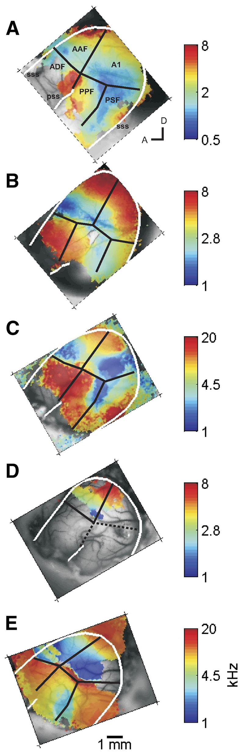
Tonotopic maps for the 5 ferrets studied herein (replotted from Nelken et al. 2004). The black lines correspond to the divisions of auditory cortex as defined by Bizley et al. (2005). The white lines highlight the border of the temporal lobe formed by the suprasylvian sulcus (sss; see A) and also indicate the location of the pseudosylvian sulcus (pss; see A). A: ferret 230 (F0230). B: F0234. C: F0242. D: F0253. E: F0256. A1, primary auditory cortex; AAF, anterior auditory field; ADF, anterior dorsal field; PPF, posterior pseudosylvian field; PSF, posterior suprasylvian field; A, anterior; D, dorsal.

Recordings were performed in a purpose-built, light- and soundproof, double-walled sound-attenuated chamber. After imaging data collection was completed the glass cover and silicone oil were removed from the chamber and agar (2% in physiological saline) was placed over the surface of the cortex for electrophysiological recordings with glass-coated tungsten electrodes.

Stimulation protocols

Stimuli consisted of sequences of short (30- to 50-ms) consecutive sound bursts with a parameter that changed gradually over the duration of the sequence. Typically, sequences were 10–14 s long. Identical sequences were repeated in a continuous loop to produce continuous stimulation lasting 150 s. Usually, these continuous stimulation periods were repeated 10 times. Thus a total of about 25 min of data were collected to map each stimulus parameter.

To reveal the tonotopic organization of the temporal cortex we used pure-tone sequences of gradually rising or falling frequency. The resulting tonotopic maps, previously published in Nelken et al. (2004), were subsequently verified with electrophysiological recordings (Bizley et al. 2005). The tonotopic maps of all the animals used in this study are reproduced in Fig. 1 for comparison with the complex sound maps generated here. The figure shows color-coded surface maps of the left temporal cortices, oriented so that the rostral part is seen on the left and the dorsal part is shown topmost in each figure panel. Maps shown in the following text (Figs. 2, 4, 7, and 8) are oriented in the same way.

Fig. 2.

Areas showing significant (F >2) modulation by periodic stimuli for 2 animals. A–C: F0230, areas modulated by sinusoidally amplitude modulated (SAM) tones (A), high-pass click trains (B), and high-pass iterated ripple noise (IRN) (C). D and E: F0242, areas modulated by SAM tones (D), high-pass click trains (E), and high-pass IRN (F). The magenta lines represent the 4-kHz isofrequency contours extracted from the frequency maps of the respective animals (Fig. 1, A and C , respectively).

Fig. 4.

Parameter-sensitivity maps for periodic stimuli in 2 animals. The panels represent the trigger periods at all pixels with significant modulation of the optical signal. A–C: F0242, maps for SAM tones (A), high-pass click trains (B), and high-pass IRN (C) (corresponding to activation areas in Fig. 2, D–F , respectively. The frequency organization of the auditory cortex in this animal is shown in Fig. 1C ). D–F: F0253, maps for SAM tones (D), highpass click trains (E), and high-pass IRN (F) for F (the frequency organization of the auditory cortex in this animal is shown in Fig. 1D ). The color scale is given in terms of “pitch” (1/period).

Fig. 7.

A–C: maps of zero crossings of the RMFs in response to tone sequences presented in 3 different aural configurations. The 3 maps are plotted with the same color scale. A: contralateral. B: ipsilateral. C: diotic. D and E: scatterplots comparing the zero crossings in the different aural configurations.

Fig. 8.

A: maps of reflectance changes evoked by noise in 3 aural configurations for F0234. Only pixels at which the optical signal was >1 SD away from its mean reflectance in silence are displayed. Activated regions have low reflectance (blue). In the difference map diotic-contra, only pixels in which both reflectance values were >1 SD away from their respective mean reflectance in silence are displayed. Positive (red) values correspond to larger contralateral activation. The magenta lines are the 4-kHz isofre-quency lines, extracted from the tonotopic map for this animal (Fig. 1B ). Color scale for the single conditions (contralateral, ipsilateral, and diotic) is saturated at 15%, for the difference map at 4.5%. B: the same data for F0242. The tonotopic map is in Fig. 1C . Color scale for the single conditions is saturated at 10%, for the difference map at 3%. C: the same data for animal F0256. The tonotopic map is in Fig. 1E . Color scale for the single conditions is saturated at 15%, for the difference map at 4.5%.

To study binaural interactions, broadband noise stimuli were presented in different aural configurations using a standard fixed-stimulus technique, where each binaural stimulus was presented individually, with long intervals between stimuli to let the responses die out before the next stimulus. Data were also collected using the continuous acquisition paradigm with sequences of noise bursts with systematically varying interaural level difference (ILD).

For the fixed-stimulus experiments, the time between stimuli was 17.5 s and each stimulus was presented 64 times. These values are similar to those used by Versnel et al. (2002) for collecting tonal maps. Stimuli consisted of broadband noise bursts, presented either to the contralateral ear or to the ipsilateral ear alone, or to both ears diotically. The total stimulus level was about 75 dB SPL in each ear.

For the continuous acquisition experiments, the ILD sequences consisted of 50-ms frozen Gaussian noise bursts delivered at a rate of 2 s⁻¹. The noise waveform delivered to each ear was identical, except that the noise was scaled to produce systematically varying stimulus intensities in each ear. The average binaural level was constant at about 75 dB SPL, but the ILD varied systematically over a ±28-dB range, changing at a rate of 4 dB s⁻¹, so that it took a total of 14 s for the noise bursts to cycle from 28 dB left ear louder to 28 dB right ear louder and back to the left.

To study the periodotopic organization of auditory cortex, we used three classes of stimuli: 1) sinusoidally amplitude modulated (SAM) tones with a 6-kHz carrier, 2) click trains and high-pass filtered click trains, and 3) iterated ripple noises (IRNs). Of these three classes of stimuli, only the click stimuli were strictly periodic, in the sense that they repeated with an identical waveform on every period. The individual SAM sounds had periodic envelopes, but were strictly periodic only when the modulator and the carrier were harmonically related. IRNs were created by repeatedly applying delay-and-add operations to a white-noise stimulus. IRNs were also not strictly periodic, but the repeated delay-and-add operation caused sufficient approximate periodicity to evoke a very robust pitch sensation.

Only the click trains were strictly periodic in the sense that each period is an identical copy of any other period. Nevertheless, for simplicity, all three classes of stimuli will hereafter be called “periodic stimuli.” Furthermore, the term “period” will be used interchangeably to refer to the modulator frequency of SAM tones, the click interval of click trains, or the delay period of the IRN, respectively.

Sounds whose energy resides entirely at >4 kHz do not produce reliable musical pitch in humans (Pressnitzer et al. 2001). Thus although many of these stimuli induce a pitch percept in human listeners with a pitch equal to the reciprocal of the period (the repetition rate) of the sound, some will produce stronger and more unambiguous pitch percept than others. We subsequently refer to the reciprocal of the period of a sound as its “pitch,” even when the strength of the pitch percept for the particular sound might be weak, because this allows us to distinguish clearly between the “pitch” period of a stimulus and the repetition period for repeatedly presented stimulus sequences.

The sequences of the periodic stimuli consisted of 61 sound bursts, rising in “pitch” in 60 equal steps on a logarithmic scale from 100 to 3,200 Hz. A single, fixed-sequence duration was used in each experiment, which varied from 10 to 14 s among experiments.

SAM tones were created by multiplying a 6-kHz carrier with a raised sinusoidal envelope and played at a sampling rate of 25 kHz. Click trains and high-passed click trains were created by generating click (“delta function”) sequences and filtering them through a digital four-pole Butterworth high-pass filter. The corner frequency of the high-pass filter was set at 0 (no filtering), 2, or 4 kHz. IRNs (Yost et al. 1996) were generated by adding up random Gaussian noise to itself, with a delay equal to the required period. Three delay-and-add operations were cascaded to generate the IRN. To generate filtered IRNs, the signal was filtered through a digital four-pole Butterworth high-pass filter. The click train and IRN stimuli were played at a sampling rate of 48.8 kHz. All signal processing was performed on the fly on an RP2 signal processor (Tucker-Davis Technologies, Alachua, FL).

Data collection

Intrinsic optical signals were acquired using Imager 2001 VSD+ (Optical Imaging, Mountainside, NJ). Data were collected while the cortex was illuminated by narrowband green light (wavelength, 546 nm; 50% bandwidth, 10 nm; Coherent-Ealing, Ealing Electro-Optics, Holliston, MA) directed through two fiber-optic light guides. Images were grabbed using a video camera (CS8310C, Tokyo Electronic Industries, Tokyo, Japan), mounted above the cortex and perpendicular to its surface. The area over which data were collected measured approximately 8 × 6 mm, at 1/4 or 1/9 of the maximal resolution (758 × 568 pixels). Blood vessel artifacts at the cortical surface were reduced using a macro double-lens configuration (2 × 50-mm SLR camera lenses mounted front to front; Nikon, Tokyo, Japan) with a shallow depth of field and focused 500 μm below the cortical surface. We used the VDAQ/NT data acquisition software (v1.5, Optical Imaging).

To synchronize the auditory stimulation and the optical image acquisition, we used a separate computer that collected all the necessary timing information using AlphaMap (Alpha Omega, Nazareth, Israel). A digital output signal that changed its state on every image acquisition was used to determine image acquisition times. The stimulus generation system produced two timing signals, one that was on during the actual stimulus presentation and a second one that turned on at the start of each sequence repeat. The same computer also recorded the times of every stroke of the respirator and the waveform of the ECG. The nominal period between images was 80 ms in one experiment and 240 ms in the other four experiments. The precise times of image acquisitions, as determined from the digital output of the Imager 2001 system, fluctuated somewhat around these values.

Electrophysiology

Extracellular recordings were made using fixed arrays of four tungsten-in-glass electrodes. The signals were band-pass filtered (500–5 kHz), amplified (≤ 10,000-fold), and digitized at 25 kHz. Data were collected and analyzed using BrainWare software (Tucker-Davis Technologies). Single units and small multiunit clusters were isolated from the digitized signal. Stimuli were presented pseudorandomly at a repetition rate of 1/s with 5–10 repetitions per recording. Frequency mapping was performed with pure tones ranging from approximately 0.5 to 30 kHz and approximately 10 to 90 dB SPL. Exact parameters varied between animals. The responses to pure tones have been described in Nelken et al. (2004). “Periodicity tuning curves” were recorded with 100-ms SAM tones, high-pass filtered click trains, or IRN bursts exactly like those used during imaging, with pitch values ranging from 100 to 3,200 Hz in 16 logarithmic steps.

All data presented are from units whose spike counts during the stimulus were significantly different from the spike counts in windows of the same duration just preceding stimulus onset (P < 0.05, paired t-test). Units were classified as selective if a one-way ANOVA of spike count against pitch showed a significant effect (P < 0.05).

Data analysis

The acquired images were analyzed on a pixel-by-pixel basis. Full details, including stability and reproducibility analysis, are given in Nelken et al. (2004). We refer to the time series of reflectance values observed at one particular pixel as the pixel’s “optical waveform.” Since the optical reflectance was highly smooth over the cortical surface, the images were downsampled by a factor of 3. The first step in the analysis of the optical waveform was to correct for respiration artifacts (for a full description see Nelken et al. 2004). After correction for respiratory and heartbeat artifacts, the optical waveforms were normalized by expressing them as a proportion of the average reflectance value for each pixel across the entire recording time. All further analysis was performed on the corrected, normalized frame sequences.

From the normalized signal we then calculated the stimulus-dependent reflectance modulation function (RMF) by averaging the optical waveform as a function of time during the stimulus sequence, after correction for the possible small jitter in frame acquisition times as in Nelken et al. (2004). To judge the statistical significance of the stimulus-evoked modulation, a one-way ANOVA was performed, with the time after the start of the sequence as the factor. In all figures, only pixels whose F value from the ANOVA test was >2 are displayed. The F value represents the ratio of the variance of the RMF as a function of time over the average variance of the responses to individual cycles around this mean. It is therefore a “signal-to-noise ratio” and the value of 2 is a reasonable cutoff point. The nominal significance of this F value with respect to the null hypothesis of no modulation is <0.01 for all tests performed here, and <0.0001 for the typical tests (sequences of 12 s). Because of temporal correlations in the signal, we estimated the probability of exceeding F = 2 for Gaussian processes with the same power spectrum as that of a typical optical waveform. The true significance level is 1–3% for a critical value of 2, but this probability decreases very fast with further increase in the critical value (for example, for F = 2.5 it is about 1% and for F = 3 it is <0.5%). Because the parameter maps most often contain about 5,000 pixels, we would expect, on average, about 25 “significant” pixels to arise by chance when using a criterion of F >3. In fact, the map with the smallest number of significant pixels presented herein had almost fourfold as many pixels with F >3. Thus all maps presented here have substantially more pixels with significant modulation than would be expected by chance.

To be able to derive estimates of preferred stimulus parameters from the RMF it is necessary to estimate the temporal relationship between the RMF and the start of the stimulus sequence. Our data analysis is based on the assumption that the RMF is the signature of a stereotyped response of a cortical pixel, which is “triggered” when the stimulus sequence crosses the tuning curves of the neurons in the pixel. Consequently, if we understand the (presumably fixed) temporal relationship between identifiable features of the RMF (like maxima or zero crossings) and the “trigger point” then we can deduce which stimulus parameter triggered the response.

In the simplest version of this model, the “temporal position” of the RMF relative to the start of the stimulus sequence is determined by two factors: 1) a fixed delay, which depends on the dynamics of the reflectance signal, and is expected to be on the order of about 1 s; and 2) the time from the beginning of the sequence until the trigger parameter value. If we take downward zero crossings as points of reference on the RMF, then these temporal relationships are given by the following equation

$$zc(x,y)=T+\frac{p(x,y)-p(start)}{p(end)-p(start)}D$$

where zc(x, y) is the time of the zero crossing at the pixel with coordinates x and y; T is the delay, assumed to be fixed across conditions and across the imaged area; p(x, y) is the parameter value that triggers the response; and D is the duration of the sequence that starts at parameter value p(start) and ends at parameter value p(end). Note that p(start), p(end), D, and zc(x, y) are either given or easily measured. The delay T was estimated using the pure-tone responses for each individual animal in Nelken et al. (2004) and these values were used here. Thus once the zero crossing times are identified, the trigger parameter can be computed. Errors in the estimate of T would result in a global shift of the resulting parameter map, but not of its shape.

One possible limitation of the fixed-delay approach is a potential dependence of the delay on the stimulus. For example, at a fixed sound level, some neurons show strong correlations between response magnitude and response latency (e.g., Nelken et al. 2005), and magnetoencephalography (MEG) studies have shown a correlation between the latency of some response components and the period of quasi-periodic stimuli (Krumbholz et al. 2003). However, these latency shifts are on the order of 10–100 ms and are therefore much smaller than the uncertainty in our estimates of the delay.

Statistical tests are considered significant when P < 0.05. For tests resulting in extreme values of the statistics, better bounds on the P values are reported. In some of the ANOVA tests, post hoc comparisons have been performed. These are always done using Tukey’s honestly significant difference criterion at the 0.05 level.

Results

Periodotopicity

We used three types of periodic stimuli: SAM tones, click trains, and IRN. In addition, the click trains and IRN were filtered to different degrees. Both stimulus type and filter settings influenced the optical signals. We will report first the extent of activation by each stimulus and then the properties of the resulting parameter maps.

To illustrate the extent of activation of the cortical surface by the periodic stimuli, Fig. 2 shows maps of the F values for the RMFs recorded using a sequence of SAM tones, high-passed clicks, or high-passed IRN in two animals (Fig. 2, A–C : animal F0230; Fig. 2, D–F : F0242). In all five animals, the area with significant modulation for SAM tones and the area with significant modulation for clicks were comparable in size. Whereas in two animals these areas were shifted relative to each other, as in Fig. 2, A and B , in the remaining three animals, the territories that were significantly activated by SAM tones and by high-passed clicks were much larger and overlapped significantly, as illustrated in Fig. 2, D and E . In contrast, the area with significant modulation for IRN was consistently substantially smaller (Fig. 2, C and F ).

The areas with significant modulation for SAM tones, high-passed filtered clicks, and high-passed IRN (three stimuli that have roughly similar bandwidths) were compared across all animals. There was a significant effect of stimulus type [F(2,7) = 6.65, P < 0.05, two-way ANOVA] and post hoc comparisons showed that the area activated by IRN was significantly smaller than the area activated by the SAM tones. The area activated by click trains was intermediate between the other two and not significantly different (post hoc tests at the 0.05 level) from either.

Given the tonotopic organization of much of auditory cortex, we might have expected SAM tones, the most narrowband stimuli used with most energy around 6 kHz, to activate a smaller area than the other stimuli (clicks and IRN). In fact, the opposite was observed. We therefore repeated the analysis, this time using the clicks and IRNs at all filter settings. We expected the wider bandwidth of the stimuli to cause a substantial increase in the size of significantly modulated cortical areas and make them comparable to the area significantly modulated by the SAM tones. Surprisingly, the pattern of results remained very much the same: the territories over which each of the three periodic stimuli evoked significant responses varied significantly by type [F(2,17) = 14.5, P << 0.05, two-way ANOVA on stimulus type × experiment]. Post hoc comparisons indicated that the area activated by IRN was significantly smaller than the areas activated by the click trains or SAM tones, which did not differ significantly from each other. These results suggest that SAM tones activated the cortex to a substantially greater degree than expected purely by their simple spectral structure.

The total area activated by the different types of periodic stimuli may not be a good measure for the area of a putative periodotopic map. A pitch-sensitive area should be activated by stimuli that have the right periodicity regardless of whether they contain the appropriate spectral energy according to the tonotopic map, but the periodic stimuli could activate more than just the relevant part of the periodotopic map. We therefore determined which parts of the low-frequency representation showed significant modulation when presented with the different periodic stimuli and how these varied depending on stimulus type and on filter settings.

When comparing the SAM, clicks, and IRN without filtering (so that the clicks and IRNs had low-frequency energy), the overlap between the low-frequency representation (<4 kHz, the 4-kHz isofrequency contours are marked on Fig. 2) defined by responses to tonal stimuli and the areas significantly modulated by the periodic stimuli depended highly significantly on the stimulus type [F(2,3) = 42.7, P < 0.05], with IRN showing substantially more overlap (almost 20% more on average) than the SAM tones or the click trains.

However, when comparing overlap with the low-frequency representation for the high-passed stimuli, the finding was different. There was still a significant effect of stimulus type [SAM tones, high-passed clicks, and high-passed IRN; F(2,12) = 4.32, P < 0.05]. However, post hoc comparisons showed that, for these stimuli, the fraction of SAM tone responses in the low-frequency representation (54% on average) was significantly larger than that of the IRN stimuli (11% on average). The click stimuli had intermediate overlap values (38% on average) that were not significantly different from either of the other two stimuli.

In summary, the three periodic stimuli behaved differently in terms of the activated area and its dependence on high-pass filtering. On average, IRN stimuli activated a significantly smaller area than the other two stimuli and the activated areas overlapped substantially with low-frequency regions when the stimulus was unfiltered (and therefore contained low frequencies) but much less so when it was high-pass filtered. Click stimuli activated larger areas than those activated by the IRN in spite of the similar bandwidth. Furthermore, on average, filtering did not have much effect on the size of the activated areas, although in at least one animal (F0230) the areas activated by high-passed clicks did not overlap the low-frequency representation, as expected from the spectral structure of these stimuli. Finally, SAM tones activated the largest areas, even though their bandwidth was the smallest and the acoustic stimulus consisted only of high-frequency components.

Turning now to the parameter sensitivity of the responses, the RMFs in response to the periodic stimuli were much the same as the RMFs in response to the tones. Figure 3 shows RMFs collected from the same pixels for different periodic stimuli (animal F0242): SAM tones (Fig. 3A ), clicks (with no filtering) (Fig. 3B ), and IRN (also without filtering) (Fig. 3C ). These RMFs were collected along a line crossing the low-frequency representation in A1, where a periodotopic map might be expected to exist. Clearly, all three stimuli caused a significant modulation of the reflectance in at least part of this territory. However, the details of the modulation differed from stimulus to stimulus. In particular, markers for the stimulus sensitivity of the optical signal such as the maximum, minimum, and the downward zero crossing of the RMFs were very different for the three stimuli. Here, the downward zero crossings (magenta lines in Fig. 3, A–C ) are the preferred marker for activation of the tissue (for a discussion of this choice see Nelken et al. 2004). For the SAM stimuli, the zero crossings occurred relatively early in the sequence, for the clicks they occurred at about the middle, and for the IRN they occurred late in the sequence. Thus in this animal, whereas the optical signal was sensitive to the periodicity of each of the three stimulus types, this sensitivity was specific to each stimulus.

Fig. 3.

Examples of reflectance modulation functions (RMFs) collected along the same line on the cortical surface (F0242, inset) using 3 different types of periodic stimuli. Red indicates increased reflectance relative to the mean; blue indicates decreased reflectance, signaling increased blood volume in the tissue. A: SAM tones (color scale saturation: 2.2%). B: click trains (unfiltered, color scale saturation: 1.8%). C: IRN (unfiltered, color scale saturation: 1.2%). Magenta lines in A–C correspond to the downward zero crossing in the RMF.

Parameter-sensitivity maps were generated by inverting Eq. 1. T was the delay estimated for the tonotopic maps for each animal in Nelken et al. (2004). Examples of such maps are shown in Fig. 4. The most striking finding illustrated in Fig. 4 is the general incompatibility between the maps generated using different periodic stimuli. For example, the wide territory in which the optical signal was modulated by SAM tones in Fig. 4A (animal F0242) contained a representation of both high- and low-pitch values. Low-pitch values were mainly represented in low-frequency areas, whereas high-pitch values were mainly represented in high-frequency areas (see Fig. 1C for the tonotopic maps in this animal). For the high-pass click train stimuli, there was a similar arrangement but the high-frequency areas showed sensitivity to much higher pitch values (Fig. 4B ). The IRN stimuli (Fig. 4C ) significantly modulated the optical signal only in high-frequency A1 and produced no significant pitch-related modulations in widespread areas that were well modulated by SAM tones and click trains. The discrepancy was even more pronounced in the anterior part of the primary fields near the tip of the ectosylvian gyrus. Here, the SAM tones showed preference to low pitches even in high-frequency areas, whereas the high-pass click trains showed sensitivity to higher pitches at the same locations; IRNs did not show any sensitivity.

In a second animal (F0253), the SAM tones again caused modulation over an extensive cortical territory (the tonotopic maps in the primary areas for this animal, shown in Fig. 1D , occupied a much smaller area). For the SAM tones, the periodotopic gradient (Fig. 4D ) is again approximately parallel to the tonotopic gradient (as in animal F0242, Fig. 4A ). In this case, however, the high-pass click trains had almost constant trigger periods along the same line (Fig. 4E ). The high-pass IRN stimuli also had an almost constant trigger period, but at a much shorter value (Fig. 4F ). These results are therefore consistent with the data from ferret F0242, in that different stimuli with the same period evoked different patterns of activity in the cortex.

In general, maps derived from the responses to SAM tones and unfiltered click trains shared the greatest similarity; this similarity was most evident in the low-frequency tonotopic areas. However, unfiltered IRNs invariably gave rise to totally different pitch representations in the same areas.

Electrophysiological responses to periodic stimuli

To validate the optical maps, we compared the optical data with electrophysiological recordings of multiunit spiking activity in response to the same stimuli. Overall, 62 recording locations in four of the five ferrets were tested with some or all of the three types of periodic stimuli (SAM tones, IRN, and clicks), giving rise to 114 comparisons of electrophysiological and optical responses. Representative examples of electrophys-iological responses are shown in Fig. 5. Responses to high-pass click trains almost always showed sensitivity to the click repetition rate, although this sensitivity was almost exclusively high-pass. Responses to IRN were only very rarely selective to pitch, although the IRN stimuli often evoked significant responses. The responses to the SAM tones were intermediate, with about half the number of recording sites showing significant tuning to pitch. As expected from the optical maps, there was no statistically significant association between the selectivity of the same cluster to the different stimulus types. For example, among the 12 clusters tested with both SAM tones and clicks, 4 had significant modulation by clicks but not by SAM tones; 2 had significant modulation by SAM tones but not by clicks; and 6 had significant modulation by both clicks and SAM tones. This is nonsignificant at the 0.05 level by Fisher’s exact test.

Fig. 5.

Comparison of electrophysiological and optical responses. The color maps give multiunit spike rates as a function of stimulus pitch (y-axis) and time poststimulus onset (x-axis). The horizontal magenta lines indicate the trigger pitch of the optical signal at the corresponding location, for those cases in which the RMF had significant modulation. The number in the title is the F value for the RMF recorded at the electrode location earlier in the same experiment. The black lines indicates stimulus duration. A and B: responses of the same multiunit cluster to high-pass click trains (A) and high-pass IRN (B). C and D: responses of another cluster to high-pass click trains (C) and SAM tones (D). E and F: responses of a third cluster to SAM tones (E) and high-pass IRN (F).

The depth of modulation of the optical signal due to pitch variation tended to be larger in those pixels where electrophysiological recordings exhibited selectivity to pitch for the same type of stimulus (compare Fig. 5A , where both the electrophysiological response was selective to pitch and the optical modulation was large, and Fig. 5B , where the electrophysiological response, although significant, was nonselective to pitch and the optical modulation was weak). Figure 6A shows the number of cases that had nonsignificant modulation (F <2) and significant modulation (F ≥2) of the optical signal, separately for cases with significant versus nonsignificant selectivity of the spiking responses. Cases with significant pitch selectivity of the spiking responses (54/114) had a clear tendency for significant modulation of the optical signal by the same type of stimulus (44/54 cases, 81%). Similarly, cases with nonsignificant selectivity to pitch in the electrophysiological responses (60/114) tended to have nonsignificant modulation of the optical signal (45/60 cases, 75%). Stated alternatively, among 69 cases that had significant modulation of the optical signal, 44 had a significant modulation of the spike rate as a function of periodicity; and among the 55 cases with nonsignificant modulation of the optical signal, 45 cases also had a nonsignificant modulation of the spike rate (64 and 82%, respectively). The tendency of recording locations to have both significant modulation of the optical signal and a significant modulation of the multiunit responses by periodicity (and vice versa) was highly significant (χ² = 36, df = 1, P << 0.01).

Fig. 6.

Relationships between electrophysiological and optical responses. A: histograms comparing the number of recording locations where spike counts did (white bars) or did not (black bars) depend significantly on stimulus pitch. Recording sites are split into groups depending on whether the optical RMFs recorded at the same location were significantly modulated by pitch. Pitch-selective electrophysiological responses are clearly associated with RMFs exhibiting significant pitch modulation. B: distribution of number of “hits,” cases in which the trigger pitch of the RMF also evoked maximal spiking responses, in the surrogate data (see text for details). The actual measured value is marked with an arrow.

There was also a significant association between the trigger pitch for the optical and electrophysiological responses. Thus the pitch trigger value corresponded to the stimulus pitch evoking the largest spiking response in 10/44 (23%) cases with both significant modulation of the optical signal and significant selectivity of the spiking responses. The significance of this association was checked by calculating the same percentage while randomly permuting the trigger pitch values among the spiking responses. Only 1.4% (140/10,000 permutations) had ≥10 of the trigger values at the largest spiking responses (Fig. 6B ). In another 10 locations, the pitch trigger value fell within one octave of the stimulus pitch that evoked the largest spiking response. In 9 of these 10 locations, the stimulus pitch that evoked the largest spiking response was lower than the trigger pitch value, so that the increase in neural activity presumably occurred shortly before the corresponding decrease in reflectance. The excess of this configuration was significant (χ² = 6.4, df = 1, P < 0.05). Thus a similarity between the electrophysiological and optical selectivity was found in about half of the cases (20/44, 45%). In the other cases (24/44), the difference between the trigger pitch and the stimulus pitch that evoked the largest spiking response was >1 octave, precluding a meaningful comparison between them.

Binaural responses

Binaural interactions were studied using three paradigms. The first paradigm tested the stability of the tonotopic organization with respect to different aural configurations. The other two paradigms used broadband noise stimulation and were designed to demonstrate correlates of EE and EI interactions in the optical signal. For this purpose, both fixed-stimulus paradigms and sequences of broadband noise bursts with varying ILDs were used.

First, tone sequences were used in three aural configurations: right (contralateral) ear alone, left (ipsilateral) ear alone, and diotically. Figure 7 presents three zero-crossing maps for the same tone sequence (upward frequency sweep, 14 s) at three aural configurations (animal F0256). The similarity between the three maps is clear and, although there are some differences (e.g., in the location of the discontinuity at the center of the map), these results show that the tonotopic organization revealed by optical imaging is largely invariant with respect to aurality, as expected from previous electrophysiological evidence. For more quantitative comparisons, the zero crossings estimated from the maps for the contralateral stimulation (Fig. 7A ) and ipsilateral stimulation (Fig. 7B ) for each pixel are displayed as a scatterplot in Fig. 7D . A similar scatterplot for the zero crossings estimated from the contralateral stimulation and the diotic stimulation (Fig. 7C ) is displayed in Fig. 7E . In both cases, there are only small shifts of the zero crossings. These shifts, although small, were systematic: the zero crossings for contralateral stimulation occurred somewhat later than for the other two configurations. Such shifts could be due to differences in the response latency (T in Eq. 1) between the difference aural configurations, but there were insufficient data to confirm this. The clusters of points away from the diagonal (in the top left corner for Fig. 7D and in the bottom right corner for Fig. 7E ) represent pixels in which the phase wrapped back to 0 in one aural configuration but not in the other. In spite of these spots, the correlation coefficients between the maps in Fig. 7 are high: 0.7 (contra to ipsi) and 0.48 (contra to diotic).

Tone sequences of various durations and aural configurations were used in two experiments. Overall, the correlation coefficients between the zero-crossing maps were high (mean ± SD: 0.73 ± 0.2, 12 comparisons; range 0.38–0.99). Thus the example in Fig. 7 is typical.

Although the tonotopic map appears to be very similar in different aural configurations, the size of the response can show effects of binaural interactions. To look for correlates of binaural interactions in the optical signals, we used broadband noise bursts in contralateral, ipsilateral, and diotic configurations in a fixed-stimulus design. Figure 8 shows activation maps for broadband noise in the three aural configurations using the standard fixed-stimulus paradigm, for three of the five animals for which such data were collected (A: F0234; B: F0242; C: F0256). The overall sound level for the noise stimuli was the same as that of the tone stimuli (~70 dB SPL). Broadband noise activated large cortical territories, usually encompassing all the areas that were activated by any of the other sound stimuli tested. Contralateral stimulation elicited the strongest responses in all animals and ipsilateral stimulation elicited the weakest responses of the three configurations, although these responses were still substantial. Diotic stimulation elicited intermediate responses in all animals except one, in which these were slightly weaker on average than the ipsilateral responses. All of these differences were statistically significant [F(2,445892) = 7.109, P << 0.05; two-way ANOVA on aural condition × experiment; only pixels with significant deviation from baseline were used; all post hoc comparisons were highly significant]. These results suggest that, although ipsilateral stimulation on its own can evoke quite substantial optical signals, in the diotic condition the overall net effect of ipsilateral stimulation on the optical responses is suppressive.

In spite of the significant differences in the magnitude of the reflectance changes between the aural conditions, the observed differences in the size of the activated areas (defined as the fraction of the imaged area where the responses were larger than twice their SD) were not statistically significant.

The right column of Fig. 8 presents maps of the difference between reflectance changes due to diotic and contralateral stimulation. It is tempting to identify pixels with lower contralateral than diotic reflectance (red in these maps) as containing mostly neurons with EI neurons and pixels with comparable or lower diotic than contralateral reflectance as containing mostly EE neurons. However, optical signals, which are due to metabolic coupling with neural activity, do not distinguish between excitatory and inhibitory inputs: lower reflectance does not necessarily mean larger spiking responses. Thus even areas in which the diotic reflectance changes were similar to or lower than the contralateral reflectance changes could have inhibitory binaural characteristics. For example, if the inhibitory interaction occurred in the cortex itself, diotic reflectance changes could be due to larger neuronal activity that sums together both excitatory (contralateral) and inhibitory (ipsilateral) inputs. Similarly, areas showing contralateral dominance could show higher diotic spiking responses, in which case the contralateral reflectance changes might actually indicate inhibitory, rather than excitatory, inputs.

In spite of these interpretation problems, based on a criterion of contralateral dominance, presumptive “EI regions” can be seen in all three maps (and also in the other two animals). However, these regions were not oriented orthogonal to the isofrequency contours (e.g., the 4-kHz contours extracted from the tonotopic maps are displayed in Fig. 8). In all three animals, the areas showing stronger contralateral than diotic responses largely avoided the high-frequency region of the primary fields and instead dominated the low-frequency regions of the maps. The contralateral-diotic contrast was significantly larger (contralateral-dominated) in the low-frequency regions than in the high-frequency region (t = –2.87, df = 4, P < 0.05, paired t-test on the mean activation values below and above 4 kHz in the five animals). Although the contralateral-dominated bands largely avoided high-frequency A1/anterior auditory field (AAF), they did extend into the high-frequency regions of the non-primary fields, but with some variation between animals. For example, in Fig. 8, A and C , such regions are seen on the posterior ectosylvian gyrus, whereas in Fig. 8B a possible EI region is seen on the anterior ectosylvian gyrus.

Nevertheless, there are clear changes in the contralateral dominance of the optical responses along isofrequency contours. Such changes occurred in all three examples displayed in Fig. 8 along the 4-kHz contour in A1/AAF. For example, in Fig. 8A the posterior end of the 4-kHz contour traversed a presumed EI region, then a region with larger diotic reflectance changes (blue), which may represent an EE region, and finally the 4-kHz isofrequency contour traversed a region with stronger contralateral signals, again presumably indicating EI responses. This sequence corresponds well to the binaural organization reported by Kelly and Judge (1994) in some ferrets. It is only by observing the large-scale organization of the presumed binaural responses, made possible by the use of optical imaging, that the breakdown of the orthogonal relationships between binaural interaction bands and isofrequency contours can be detected.

To study the large-scale binaural organization with higher resolution, we used ILD sequences. The ILD values moved between values of +28 dB (contralateral ear louder) to –28 dB (ipsilateral ear louder). With these stimuli, one might expect EI regions to have activation peaks at contralateral ILDs and activation minima at ipsilateral ILDs. EE regions could show any of a number of possible patterns depending on the details of the interaction between the ears, including reduced modulation (if the optical signals produced by stimulating the two ears separately sum up linearly) or period halving (if the optical signal corresponded to the maximum overall sound level at either ear, which occurs twice per period).

Responses to ILD sequences and to the constituent contralateral and ipsilateral monaural sequences were collected in three animals (F0242, F0253, and F0256). RMFs at the three aural configurations in one animal (F0242), collected along the same line on the cortical surface, are shown in Fig. 9A . The RMFs collected with ipsilateral and contralateral stimulation are roughly in counterphase to each other, and the RMF collected in the binaural stimulation condition (bottom) was smaller than either of the monaural RMFs.

Fig. 9.

A: RMFs recorded in response to level changes in the contralateral, ipsilateral, or both (binaural) ears along a line on the cortical surface (animal F0242). The color scale is saturated at 3% (same value for all 3 panels). B and C: scatterplots of the amplitudes of the RMFs for all the pixels with significant modulation (same animal as in A). D– F: histograms of the phase of the RMFs for contralateral (blue) and ipsilateral (red) stimulation. Each panel corresponds to the data from a different animal (D: F0242; E: F0253; F: F0256). Only data from pixels with significant modulation in both conditions are used.

Surprisingly, for all experiments, the RMFs recorded in response to the ipsilaterally presented level sequences tended to have the largest amplitudes, followed by the contralateral RMFs (Fig. 9, B and C ). The binaural RMFs were always the smallest. This result was confirmed by a two-way ANOVA test [aural condition × experiment; effect of aural condition: F(2,12647) = 55, P << 0.05]. Post hoc comparisons showed that all differences were statistically significant. Similarly, the territory size over which the RMFs had significant modulation followed the same order: the largest territories occurred for the ipsilateral stimulation and the smallest territories with significant modulation were found with binaural stimulation.

Figure 9, D–F shows the histogram of the phases of the fundamental period of the RMFs in the two monaural configurations for the three animals. The difference between the peaks of the two distributions is roughly π radians, corresponding to the antiphase relationships of the stimulation sequences in the two cases. Thus it seems that the two monaural conditions were essentially equivalent in terms of the phase of the optical signal: large optical signal amplitude was roughly related to high stimulus level.

The small deviations in the phase of the RMFs observed in Fig. 9A may be interpreted naturally as differences in thresholds to broadband noise bursts along the cortical surface. The data in Fig. 9A suggest that these differences were correlated between the two ears, so that earlier phases for contralateral and ipsilateral stimulations co-occurred. This was especially true for two animals (F0242 and F0253), where the correlation coefficient between the phase of the responses to contralateral and ipsilateral stimulation was >0.8. For the third animal, the range of phases was substantially smaller (see Fig. 9F ) and the correlation coefficient, although highly significant, was substantially smaller (0.3). Topographic maps of these phases did not show any reproducible behavior across animals (data not shown).

One possible explanation for the relatively small modulation of the optical signal during binaural stimulation with ILD sequences is that the activation level in the binaural condition was roughly the sum of the two monaural conditions and thus was large when either ear was stimulated at high levels. In this case, it would be expected that the mean reflectance level in the binaural condition would be the smallest (corresponding to the largest blood flow) among the three aural configurations. To test this, the reflectance in each pixel, averaged across the whole stimulation period, was compared between aural configurations. The mean reflectance level was indeed different in the three conditions [two-way ANOVA on aural condition × animal, F(2,23344) = 215, P << 0.001], but post hoc comparisons showed that the mean reflectance was largest (instead of smallest) in the binaural condition, corresponding to the lowest amount of blood flow.

It is possible that the smaller modulation observed with binaural stimulation is due to approximately linear summation of the processes causing the reflectance changes in response to monaural stimulation. In one animal (F0242) the binaural RMFs could be accounted for rather well by simple linear summation of the monaural RMFs (Fig. 10A ). The arithmetic sum of the two monaural RMFs (continuous cyan line) is a reasonable approximation to the binaural RMF (dashed black line). This was not the case, however, in the other two animals (Fig. 10, B and C ).

Fig. 10.

Prediction of the binaural response as a sum of the monaural responses. Data from 3 animals are shown (A: F0242; B: F0253; C: F0256). The top panel shows examples of RMFs measured in response to contra (dashed blue), ipsi (dashed green), and binaural (dashed black) stimulation. In addition, 2 types of predictions are shown: simple linear sum of the monaural responses (continuous, cyan) and an optimized weighted sum of the monaural responses (continuous, magenta). The histograms of the prediction errors normalized by the mean energy of the 2 monaural RMFs at each pixel, are shown below. Prediction weights (computed from the data of all pixels with significant modulation; see main text). A: contralateral weight: 0.77, ipsilateral weight: 0.56. B: contralateral weight: 0.05, ipsilateral weight: –0.18. C: contralateral weight: 0.41, ipsilateral weight: 0.10.

The goodness of fit of the approximation was quantified by the sum of squared differences (energy of the difference) between the predicted and measured RMFs, divided by the mean energy of the two monaural RMFs used to form the prediction. In animal F0242, the histogram of prediction errors (Fig. 10A , bottom, cyan) showed relatively small errors (its median is at 0.37, corresponding to an error of approximately one third of the mean energy of the monaural RMFs). In the other two animals, however, a simple summation of monaural RMFs often gave quite a poor approximation of the binaural response (Fig. 10, B and C , cyan histograms). In both cases, in many pixels the errors of this fit were >1, so that the fit error was often as large as or larger than the individual responses composing it.

To improve the linear prediction of the binaural responses, we tried to fit the binaural responses by a weighted sum of the monaural responses. The fit was done by least squares, over all pixels at which both of the monaural conditions showed significant modulation, and using all time lags at those pixels. This substantially improved predictions in all cases (compare the magenta and cyan lines in Fig. 10, top panels and the cyan and magenta histograms in the bottom panels of Fig. 10).

The weights of the two monaural RMFs (given in the legend of Fig. 10) were significantly different from 0 and the intercept was <0.0003 in all animals. In two animals (Fig. 10, A and C ), the weights were positive, consistent with a roughly linear interaction between the two monaural signals. In the third animal (Fig. 10B ), although qualitatively the RMFs behaved similarly, the phase of the binaural responses was closer to the phase of the contralateral stimulation than in the other two experiments. As a result, the regression weights in this case had opposite signs.

In summary, ipsilateral and contralateral stimulations produce roughly equivalent effects on the optical signal, whereas binaural stimulation caused smaller modulation of the signal. In two animals, a rough linearity was found in the relationships between the two monaural and the binaural responses, whereas in a third animal, the contralateral ear seemed to dominate the binaural responses.

Discussion

Periodotopic maps

The main interest in periodic stimuli stems from their relationship with the phenomenon of pitch; many periodic stimuli generate a pitch percept at their periodicity. A periodotopic organization of A1 has been suggested in imaging and magnetoencephalographic studies in humans (Langner et al. 1997; Pantev et al. 1989) and in a combined optical imaging and electrophysiological study of gerbil A1 (Schulze et al. 2002), in which responses to SAM tones are topographically organized and superimposed on the tonotopic map.

Like Schulze et al. (2002), we found that large extents of auditory cortex were activated by SAM tones. Regular progressions of the period sensitivity could also be demonstrated, but this progression appeared to run parallel to the tonotopic map, in contrast to the results of Langner et al. (1997) who reported an orthogonal arrangement of tonotopy and periodotopy in human auditory cortex. Our maps are roughly consistent with those generated by Schulze et al. (2002) in the gerbil, with long periods represented in low-frequency areas of the cortex and short periods represented in high-frequency cortex, particularly in high-frequency A1/AAF.

However, SAM tones evoke very strong combination tones through nonlinear distortion in the cochlea (Wiegrebe and Patterson 1999). Furthermore, with carriers >4 kHz, no pitch percept is created in humans when combination tones are controlled for (Krumbholz et al. 2000; Pressnitzer et al. 2001). It is therefore possible that the periodotopic maps observed in response to SAM tones, both by Schulze et al. (2002) and by us, result from combination tones, rather than sensitivity to the period of a high-frequency stimulus.

The data we collected with other periodic stimuli, filtered click trains, and IRN further suggest that the parameter maps observed with SAM tones are not “true periodotopic maps.” First, the extent of the regions showing significant modulation of the optical signal by the other periodic stimuli was often much smaller than that produced by the SAM tones. This was particularly true for the IRN stimuli, which often evoked a weak modulation in high-frequency regions only. Second, both the RMFs and the derived parameter maps were different for the different periodic stimuli. Finally, the electrophysiological responses to the different periodic stimuli were not consistent with a generalized sensitivity to stimulus period.

The simplest explanation of these findings is that none of the pixels in our functional maps exhibited a common sensitivity to the period of complex stimuli regardless of stimulus spectral content. Our results thus suggest that none of the areas of auditory cortex investigated here contained a true topographic representation of pitch.

Aural interactions in the intrinsic optical signals

In the fixed-stimulus paradigm, we found that both contralateral and ipsilateral stimulations activated the majority of the exposed area, although the optical signals evoked by contralateral stimulation were larger than those evoked by ipsilateral stimulation. This is consistent with a previous optical imaging study of ferret A1 (Mrsic-Flogel et al. 2006) and with electro-physiological data (Campbell et al. 2006; Kelly and Judge 1994; Phillips et al. 1988), suggesting that most, perhaps even all, cortical neurons receive inputs from both ears. The optical signal is presumably related to changes in blood flow associated with both excitatory and inhibitory responses. Thus the smaller diotic signal suggests that most of the suppression of contralateral responses by ipsilateral stimulation may occur subcortically. Although the magnitude of the reflectance changes produced by the different aural conditions varied over the cortical surface, our data do not support the existence of “binaural interaction bands” (Imig and Adrian 1977; Middlebrooks et al. 1980) orthogonal to the frequency gradient.

These conclusions are strengthened by the analysis of responses to the ILD sequences. Although equivalent in terms of their temporal structure, the ipsilateral responses showed greater modulation than that of the contralateral responses. This finding could be the result of higher thresholds to ipsilateral stimuli than to contralateral stimuli. Thus the contralateral stimulation levels used were likely to have been mostly above threshold, resulting in a higher mean activation level and smaller modulation of the optical signal, whereas the same range of levels in the ipsilateral ear could have been partly above and partly below threshold, resulting in a lower mean activation level, but larger modulations.

The responses to the dichotic sequences were much smaller, and covered a significantly smaller extent of cortex, than either contralateral or ipsilateral responses. This could be because contralateral and ipsilateral activities sum up, resulting in higher sustained activity level and consequently less modulation. Alternatively, it could be that the binaural interactions occur mostly below the cortical level and that the optical signals recorded from cortex show only their net result. This second interpretation is more consistent with the fixed-stimulus results, which also suggest a decrease in the total drive to the cortex with binaural stimulation. It is also consistent with the finding that the mean reflectance level for the ILD sequences was larger (consistent with smaller blood flow and therefore less neural activity) with dichotic stimulation than in either monaural case.

The major previous study of binaural organization in the ferret was published by Kelly and Judge (1994). There are many correspondences between the conclusions of that study and the current one. Like the current report, Kelly and Judge (1994) reported a preponderance of binaural suppression over binaural facilitation, certainly with respect to the cat, where EE clusters are the majority in essentially all studies (e.g., Matsubara and Phillips 1988; Reale and Kettner 1986; Rotman et al. 2001). They also reported clustering of the binaural responses in “EI” and “EE” bands, similarly to the areas of contralateral dominance, presumably EI, reported here (Fig. 8). However, in contrast with the data presented herein, Kelly and Judge (1994) interpreted their findings as demonstrating the presence of binaural interaction bands that are orthogonal to the isofrequency contours.

There are several methodological differences between the study of Kelly and Judge (1994) on the one hand and the current paper on the other. Perhaps the most important difference is that here we mapped a much larger extent of auditory cortex. Kelly and Judge (1994) reported one map that covers most of what is considered here as high-frequency A1 and AAF. This map is rather similar to the example in Fig. 8A , with stronger contralateral dominance in the posterior and anterior sections of the mapped area and diotic dominance in the middle of the field. Otherwise, their maps cover rather small parts of the middle ectosylvian gyrus (MEG), in many cases a single isofrequency contour, emphasizing high frequencies (>10 kHz). In particular, Kelly and Judge (1994) did not map the low-frequency areas where we suggest the presence of strong contralateral dominance. Thus whereas in those parts of A1 and AAF that were mapped in both studies the results of each study are compatible, the use of optical imaging, making it possible to map substantially larger areas of the MEG, allowed us to uncover a larger-scale organization of binaural responses.

It must be emphasized that mapping binaural interactions along a single isofrequency contour, which is the major approach used by Kelly and Judge (1994), cannot be used to argue for binaural interaction bands—for that, it is necessary to map binaural interactions over a range of frequencies. In fact, following Reale and Kettner (1986), the tendency in studies of cat auditory cortex is to describe binaural interactions as arranged in clusters rather than as bands (e.g., Matsubara and Phillips 1988; Rotman et al. 2001). The same is true in the guinea pig auditory cortex (Rutkowski et al. 2000).

Other possible reasons for differences between the study of Kelly and Judge (1994) and the present one consist of the rather coarse definition of binaural interactions: more recent studies (starting with Semple and Kitzes 1993a,b) have adopted more complex, fine-grained binaural classification schemes (e.g., in the ferret, Campbell et al. 2006). Such more refined classification could give rise to subparcellation of their binaural interaction bands, possibly disrupting the order reported by Kelly and Judge (1994). Finally, they tested binaural interactions close to threshold, whereas in this study tests were run at suprathreshold levels. It is now well established that binaural interactions are not invariant to absolute sound level (Campbell et al. 2006; Semple and Kitzes 1993a,b). Indeed, Kelly and Judge (1994) reported a number of clusters that had “mixed” binaural interactions, with EE responses at low levels and EI responses at high levels. It is possible that these mixed clusters contributed to our contralateral dominated areas. However, since only a minority of the recording sites were classified as mixed by Kelly and Judge, this is probably not a major reason for the discrepancy between the two studies.

Lack of fine-grain structure of sensory maps in auditory cortex

In areas 17 and 18 of visual cortex, optical maps of orientation selectivity show a fine-grain structure, attributed to different orientation columns within the same “hypercolumn,” which represent all the features analyzed from a small spot in the visual scene. One of the “holy grails” of research in auditory cortex, and a major rationale for the use of optical imaging, is the search for a similar fine-grain structure, which should give hints about those parameters that are coded topographically in auditory cortex.

Our results, like those of previous studies of auditory cortex using optical signals, did not reveal any clear fine structure. For all the stimuli we used, the parameter maps we measured tended to vary slowly and continuously over large cortical extents, without the spatial changes at small scales (<1 mm) typical of maps in primary visual cortex. The data shown herein were obtained with green light, which has been shown to be less effective for imaging visual cortex (Frostig et al. 1990). However, as in previous intrinsic imaging studies of auditory cortex of the cat (Spitzer et al. 2001), we did not observe stimulus-specific reflectance changes with red (700 nm) light in any of these animals. We also found that orange light (610 nm) elicited RMFs that were significantly smaller than the corresponding RMFs in green and showed much less sensitivity to stimulus frequency.

There are two possible trivial interpretations of our data. First, it is possible that we did not use the right stimuli and that another family of parametric stimuli may give rise to signals in red light and to fine structure of the optical map of auditory cortex. According to this interpretation, the sounds we used did not activate auditory cortex strongly enough and we failed to observe its true underlying functional architecture. Second, it is possible that there is a mismatch between a large size of recruitable vascular units (as in Harrison et al. 2002) and a small size of the neuronal “modules.” According to this interpretation, optical imaging of intrinsic signals is an inappropriate methodology for studying detailed organizational features of auditory cortex.

We do not believe that either of these arguments is fully valid. We observed very large responses to a range of stimuli in green light (reaching an amplitude of 15%), revealing tonotopic organization that was reproducible and consistent both across animals and with electrophysiological data. Thus the stimuli we used strongly activated auditory cortex (probably as strongly as the visual stimuli used to image visual cortex). Second, the spatial scale of binaural interaction clusters is probably the largest of all parameters mapped in auditory cortex (Rotman et al. 2001; Schreiner 1992, 1995) and there is no a priori reason why they should not be observed with optical imaging. Similarly, the periodicity map reported in the gerbil auditory cortex covers a rather large area comparable to the area of the tonotopic map and, again, there is no reason to assume that optical imaging would not be capable of resolving such a map.

The apparent absence in the tonotopic and nontonotopic fields of a systematic variation in sensitivity to either stimulus pitch or to the binaural properties of the stimuli used in this study suggests that auditory cortex could be organized according to different principles from visual cortex. This finding now has support from studies of both auditory cortex anatomy (Harrison et al. 2002) and cortical responses to simple and complex sounds (Barbour and Wang 2002; Bar-Yosef et al. 2002; Biermann and Heil 2000; Heil 2001; Las et al. 2005; Lu et al. 2001; Nelken and Versnel 2000; Schreiner et al. 2000; Ulanovsky et al. 2003; Wang et al. 2005). In fact, Chechik et al. (2006) showed that neurons in auditory cortex of cats, even if they have the same best frequency, show a high degree of information independence when tested with complex sounds. If this is so, blood flow or other measures of metabolic demands, which are driven by the average activity of a large number of neurons, may not be good indicators of the interesting processing carried out by these neurons. Our results therefore are consistent with the view (Bar-Yosef et al. 2002) that these neurons perform high-level processing on their input, which cannot be reduced to simple feature detection and is therefore unlikely to result in systematic, topographically arranged feature maps.

References

- Bakin JS, Kwon MC, Masino SA, Weinberger NM, Frostig RD. Suprathreshold auditory cortex activation visualized by intrinsic signal optical imaging. Cereb Cortex. 1996;6:120–130. doi: 10.1093/cercor/6.2.120. [DOI] [PubMed] [Google Scholar]
- Barbour DL, Wang X. Temporal coherence sensitivity in auditory cortex. J Neurophysiol. 2002;88:2684–2699. doi: 10.1152/jn.00253.2002. [DOI] [PubMed] [Google Scholar]
- Bar-Yosef O, Rotman Y, Nelken I. Responses of neurons in cat primary auditory cortex to bird chirps: effects of temporal and spectral context. J Neurosci. 2002;22:8619–8632. doi: 10.1523/JNEUROSCI.22-19-08619.2002. [DOI] [PMC free article] [PubMed] [Google Scholar]
- Biermann S, Heil P. Parallels between timing of onset responses of single neurons in cat and of evoked magnetic fields in human auditory cortex. J Neurophysiol. 2000;84:2426–2439. doi: 10.1152/jn.2000.84.5.2426. [DOI] [PubMed] [Google Scholar]
- Bizley JK, Nodal FR, Nelken I, King AJ. Functional organization of ferret auditory cortex. Cereb Cortex. 2005;15:1637–1653. doi: 10.1093/cercor/bhi042. [DOI] [PubMed] [Google Scholar]
- Bizley JK, Walker K, King AJ, Schnupp JWH. Behavioural and neural measures of pitch discrimination in ferrets. Assoc Res Otolaryngol Abstr. 2007;398 [Google Scholar]
- Campbell RA, Schnupp JW, Shial A, King AJ. Binaural-level functions in ferret auditory cortex: evidence for a continuous distribution of response properties. J Neurophysiol. 2006;95:3742–3755. doi: 10.1152/jn.01155.2005. [DOI] [PMC free article] [PubMed] [Google Scholar]
- Chechik G, Anderson MJ, Bar-Yosef O, Young ED, Tishby N, Nelken I. Reduction of information redundancy in the ascending auditory pathway. Neuron. 2006;51:359–368. doi: 10.1016/j.neuron.2006.06.030. [DOI] [PubMed] [Google Scholar]
- Dinse HR, Godde B, Hilger T, Reuter G, Cords SM, Lenarz T, von Seelen W. Optical imaging of cat auditory cortex cochleotopic selectivity evoked by acute electrical stimulation of a multi-channel cochlear implant. Eur J Neurosci. 1997;9:113–119. doi: 10.1111/j.1460-9568.1997.tb01359.x. [DOI] [PubMed] [Google Scholar]
- Frostig RD, Lieke EE, Ts’o DY, Grinvald A. Cortical functional architecture and local coupling between neuronal activity and the microcirculation revealed by in vivo high-resolution optical imaging of intrinsic signals. Proc Natl Acad Sci USA. 1990;87:6082–6086. doi: 10.1073/pnas.87.16.6082. [DOI] [PMC free article] [PubMed] [Google Scholar]
- Harel N, Mori N, Sawada S, Mount RJ, Harrison RV. Three distinct auditory areas of cortex (AI, AII, and AAF) defined by optical imaging of intrinsic signals. Neuroimage. 2000;11:302–312. doi: 10.1006/nimg.1999.0537. [DOI] [PubMed] [Google Scholar]
- Harrison RV, Harel N, Kakigi A, Raveh E, Mount RJ. Optical imaging of intrinsic signals in chinchilla auditory cortex. Audiol Neurootol. 1998;3:214–223. doi: 10.1159/000013791. [DOI] [PubMed] [Google Scholar]
- Harrison RV, Harel N, Panesar J, Mount RJ. Blood capillary distribution correlates with hemodynamic-based functional imaging in cerebral cortex. Cereb Cortex. 2002;12:225–233. doi: 10.1093/cercor/12.3.225. [DOI] [PubMed] [Google Scholar]
- Heil P. Representation of sound onsets in the auditory system. Audiol Neurootol. 2001;6:167–172. doi: 10.1159/000046826. [DOI] [PubMed] [Google Scholar]
- Hess A, Scheich H. Optical and FDG mapping of frequency-specific activity in auditory cortex. Neuroreport. 1996;7:2643–2647. doi: 10.1097/00001756-199611040-00047. [DOI] [PubMed] [Google Scholar]
- Imig TJ, Adrian HO. Binaural columns in the primary field (A1) of cat auditory cortex. Brain Res. 1977;138:241–257. doi: 10.1016/0006-8993(77)90743-0. [DOI] [PubMed] [Google Scholar]
- Kalatsky VA, Polley DB, Merzenich MM, Schreiner CE, Stryker MP. Fine functional organization of auditory cortex revealed by Fourier optical imaging. Proc Natl Acad Sci USA. 2005;102:13325–13330. doi: 10.1073/pnas.0505592102. [DOI] [PMC free article] [PubMed] [Google Scholar]
- Kalatsky VA, Stryker MP. New paradigm for optical imaging: temporally encoded maps of intrinsic signal. Neuron. 2003;38:529–545. doi: 10.1016/s0896-6273(03)00286-1. [DOI] [PubMed] [Google Scholar]
- Kelly JB, Judge PW. Binaural organization of primary auditory cortex in the ferret (Mustela putorius) J Neurophysiol. 1994;71:904–913. doi: 10.1152/jn.1994.71.3.904. [DOI] [PubMed] [Google Scholar]
- Kelly JB, Sally SL. Organization of auditory cortex in the albino rat: binaural response properties. J Neurophysiol. 1988;59:1756–1769. doi: 10.1152/jn.1988.59.6.1756. [DOI] [PubMed] [Google Scholar]
- Krumbholz K, Patterson RD, Pressnitzer D. The lower limit of pitch as determined by rate discrimination. J Acoust Soc Am. 2000;108:1170–1180. doi: 10.1121/1.1287843. [DOI] [PubMed] [Google Scholar]
- Krumbholz K, Patterson RD, Seither-Preisler A, Lammertmann C, Lutkenhoner B. Neuromagnetic evidence for a pitch processing center in Heschl’s gyrus. Cereb Cortex. 2003;13:765–772. doi: 10.1093/cercor/13.7.765. [DOI] [PubMed] [Google Scholar]
- Langner G, Sams M, Heil P, Schulze H. Frequency and periodicity are represented in orthogonal maps in the human auditory cortex: evidence from magnetoencephalography. J Comp Physiol A Sens Neural Behav Physiol. 1997;181:665–676. doi: 10.1007/s003590050148. [DOI] [PubMed] [Google Scholar]
- Las L, Stern EA, Nelken I. Representation of tone in fluctuating maskers in the ascending auditory system. J Neurosci. 2005;25:1503–1513. doi: 10.1523/JNEUROSCI.4007-04.2005. [DOI] [PMC free article] [PubMed] [Google Scholar]
- Lu T, Liang L, Wang X. Neural representations of temporally asymmetric stimuli in the auditory cortex of awake primates. J Neurophysiol. 2001;85:2364–2380. doi: 10.1152/jn.2001.85.6.2364. [DOI] [PubMed] [Google Scholar]
- Matsubara JA, Phillips DP. Intracortical connections and their physiological correlates in the primary auditory cortex (AI) of the cat. J Comp Neurol. 1988;268:38–48. doi: 10.1002/cne.902680105. [DOI] [PubMed] [Google Scholar]
- McAlpine D. Neural sensitivity to periodicity in the inferior colliculus: evidence for the role of cochlear distortions. J Neurophysiol. 2004;92:1295–1311. doi: 10.1152/jn.00034.2004. [DOI] [PubMed] [Google Scholar]
- Middlebrooks JC, Dykes RW, Merzenich MM. Binaural response-specific bands in primary auditory cortex (AI) of the cat: topographical organization orthogonal to isofrequency contours. Brain Res. 1980;181:31–48. doi: 10.1016/0006-8993(80)91257-3. [DOI] [PubMed] [Google Scholar]
- Mrsic-Flogel TD, Versnel H, King AJ. Development of contralateral and ipsilateral frequency representations in ferret primary auditory cortex. Eur J Neurosci. 2006;23:780–792. doi: 10.1111/j.1460-9568.2006.04609.x. [DOI] [PubMed] [Google Scholar]
- Nelken I, Bizley JK, Nodal FR, Ahmed B, Schnupp JWH, King AJ. Large-scale organization of ferret auditory cortex revealed using continuous acquisition of intrinsic optical signals. J Neurophysiol. 2004;92:2574–2588. doi: 10.1152/jn.00276.2004. [DOI] [PubMed] [Google Scholar]
- Nelken I, Chechik G, Mrsic-Flogel TD, King AJ, Schnupp JWH. Encoding stimulus information by spike numbers and mean response time in primary auditory cortex. J Comput Neurosci. 2005;19:199–221. doi: 10.1007/s10827-005-1739-3. [DOI] [PubMed] [Google Scholar]
- Nelken I, Versnel H. Responses to linear and logarithmic frequency-modulated sweeps in ferret primary auditory cortex. Eur J Neurosci. 2000;12:549–562. doi: 10.1046/j.1460-9568.2000.00935.x. [DOI] [PubMed] [Google Scholar]
- Pantev C, Elbert T, Ross B, Eulitz C, Terhardt E. Binaural fusion and the representation of virtual pitch in the human auditory cortex. Hear Res. 1996;100:164–170. doi: 10.1016/0378-5955(96)00124-4. [DOI] [PubMed] [Google Scholar]
- Pantev C, Hoke M, Lutkenhoner B, Lehnertz K. Tonotopic organization of the auditory cortex: pitch versus frequency representation. Science. 1989;246:486–488. doi: 10.1126/science.2814476. [DOI] [PubMed] [Google Scholar]
- Phillips DP, Judge PW, Kelly JB. Primary auditory cortex in the ferret (Mustela putorius): neural response properties and topographic organization. Brain Res. 1988;443:281–294. doi: 10.1016/0006-8993(88)91622-8. [DOI] [PubMed] [Google Scholar]
- Pressnitzer D, Patterson RD, Krumbholz K. The lower limit of melodic pitch. J Acoust Soc Am. 2001;109:2074–2084. doi: 10.1121/1.1359797. [DOI] [PubMed] [Google Scholar]
- Reale RA, Kettner RE. Topography of binaural organization in primary auditory cortex of the cat: effects of changing interaural intensity. J Neurophysiol. 1986;56:663–682. doi: 10.1152/jn.1986.56.3.663. [DOI] [PubMed] [Google Scholar]
- Recanzone GH, Schreiner CE, Sutter ML, Beitel RE, Merzenich MM. Functional organization of spectral receptive fields in the primary auditory cortex of the owl monkey. J Comp Neurol. 1999;415:460–481. doi: 10.1002/(sici)1096-9861(19991227)415:4<460::aid-cne4>3.0.co;2-f. [DOI] [PubMed] [Google Scholar]
- Rotman Y, Bar-Yosef O, Nelken I. Relating cluster and population responses to natural sounds and tonal stimuli in cat primary auditory cortex. Hear Res. 2001;152:110–127. doi: 10.1016/s0378-5955(00)00243-4. [DOI] [PubMed] [Google Scholar]
- Rutkowski RG, Wallace MN, Shackleton TM, Palmer AR. Organisation of binaural interactions in the primary and dorsocaudal fields of the guinea pig auditory cortex. Hear Res. 2000;145:177–189. doi: 10.1016/s0378-5955(00)00087-3. [DOI] [PubMed] [Google Scholar]
- Schreiner CE. Functional organization of the auditory cortex: maps and mechanisms. Curr Opin Neurobiol. 1992;2:516–521. doi: 10.1016/0959-4388(92)90190-v. [DOI] [PubMed] [Google Scholar]
- Schreiner CE. Order and disorder in auditory cortical maps. Curr Opin Neurobiol. 1995;5:489–496. doi: 10.1016/0959-4388(95)80010-7. [DOI] [PubMed] [Google Scholar]
- Schreiner CE, Read HL, Sutter ML. Modular organization of frequency integration in primary auditory cortex. Annu Rev Neurosci. 2000;23:501–529. doi: 10.1146/annurev.neuro.23.1.501. [DOI] [PubMed] [Google Scholar]
- Schulze H, Hess A, Ohl FW, Scheich H. Superposition of horseshoe-like periodicity and linear tonotopic maps in auditory cortex of the Mongolian gerbil. Eur J Neurosci. 2002;15:1077–1084. doi: 10.1046/j.1460-9568.2002.01935.x. [DOI] [PubMed] [Google Scholar]
- Semal C, Demany L. The upper limit of musical pitch. Music Percept. 1990;8:165–176. [Google Scholar]
- Semple MN, Kitzes LM. Binaural processing of sound pressure level in cat primary auditory cortex: evidence for a representation based on absolute levels rather than interaural level differences. J Neurophysiol. 1993a;69:449–461. doi: 10.1152/jn.1993.69.2.449. [DOI] [PubMed] [Google Scholar]
- Semple MN, Kitzes LM. Focal selectivity for binaural sound pressure level in cat primary auditory cortex: two-way intensity network tuning. J Neurophysiol. 1993b;69:462–473. doi: 10.1152/jn.1993.69.2.462. [DOI] [PubMed] [Google Scholar]
- Spitzer MW, Calford MB, Clarey JC, Pettigrew JD, Roe AW. Spontaneous and stimulus-evoked intrinsic optical signals in primary auditory cortex of the cat. J Neurophysiol. 2001;85:1283–1298. doi: 10.1152/jn.2001.85.3.1283. [DOI] [PubMed] [Google Scholar]
- Ulanovsky N, Las L, Nelken I. Processing of low-probability sounds by cortical neurons. Nat Neurosci. 2003;6:391–398. doi: 10.1038/nn1032. [DOI] [PubMed] [Google Scholar]
- Versnel H, Mossop JE, Mrsic-Flogel TD, Ahmed B, Moore DR. Optical imaging of intrinsic signals in ferret auditory cortex: responses to narrowband sound stimuli. J Neurophysiol. 2002;88:1545–1558. doi: 10.1152/jn.2002.88.3.1545. [DOI] [PubMed] [Google Scholar]
- Wang X, Lu T, Snider RK, Liang L. Sustained firing in auditory cortex evoked by preferred stimuli. Nature. 2005;435:341–346. doi: 10.1038/nature03565. [DOI] [PubMed] [Google Scholar]
- Wiegrebe L, Patterson RD. Quantifying the distortion products generated by SAM noise. J Acoust Soc Am. 1999;106:2709–2718. doi: 10.1121/1.428099. [DOI] [PubMed] [Google Scholar]
- Yost WA, Patterson R, Sheft S. A time domain description for the pitch strength of iterated rippled noise. J Acoust Soc Am. 1996;99:1066–1078. doi: 10.1121/1.414593. [DOI] [PubMed] [Google Scholar]