Binaural-Level Functions in Ferret Auditory Cortex: Evidence for a Continuous Distribution of Response Properties

Abstract

Many previous studies have subdivided auditory neurons into a number of physiological classes according to various criteria applied to their binaural response properties. However, it is often unclear whether such classifications represent discrete classes of neurons or whether they merely reflect a potentially convenient but ultimately arbitrary partitioning of a continuous underlying distribution of response properties. In this study we recorded the binaural response properties of 310 units in the auditory cortex of anesthetized ferrets, using an extensive range of interaural level differences (ILDs) and average binaural levels (ABLs). Most recordings were from primary auditory fields on the middle ectosylvian gyrus and from neurons with characteristic frequencies >5 kHz. We used simple multivariate statistics to quantify a fundamental coding feature: the shapes of the binaural response functions. The shapes of all 310 binaural response surfaces were represented as points in a five-dimensional principal component space. This space captured the underlying shape of all the binaural response surfaces. The distribution of binaural level functions was not homogeneous because some shapes were more common than others. Despite this, clustering validation techniques revealed no evidence for the existence of discrete, or partially overlapping, clusters that could serve as a basis for an objective classification of binaural-level functions. We also examined the gradients of the response functions for the population of units; these gradients were greatest near the midline, which is consistent with free-field data showing that cortical neurons are most sensitive to changes in stimulus location in this region of space.

Introduction

Neuronal sensitivity to differences in sound level at each ear provides a means by which the location of high-frequency sounds can be represented in the brain. Because the auditory cortex is required for normal directional hearing (Heffner and Heffner 1990; Kavanagh and Kelly 1987; Malhotra et al. 2004; Smith et al. 2004), a number of studies have used dichotic stimuli to measure how the responses of its neurons vary with interaural level difference (ILD). These studies have made extensive use of nominal classification schemes for data reduction purposes (Imig and Adrian 1977; Irvine 1987; Kelly and Judge 1994; Kelly and Sally 1988; Middlebrooks et al. 1980; Phillips and Irvine 1983; Reale and Kettner 1986; Rutkowski et al. 2000; Zhang et al. 2004). Thus neurons were assigned to classes on the basis of their responses to monaural stimulation of the contralateral and ipsilateral ears and then typically subclassified according to the binaural interactions of the monaural responses. For example, the occurrence of nonlinear summation of the monaural inputs would be classed as a “facilitatory” interaction. The complexity of binaural stimulus sets has increased over time, with recent work using extensive two-dimensional (2D) stimulus grids in which ILDs were recorded over a broad range of average binaural sound levels (ABLs) (Irvine et al. 1996; Semple and Kitzes 1993a,b; Zhang et al. 2004). Such stimuli, having greater degrees of freedom, revealed a fascinating diversity of responses that was not evident with one-dimensional ILD functions. In the light of this complexity, the relatively simple binaural classification schemes originally devised are no longer adequate, and the functional organization of auditory cortex with respect to binaural response properties needs to be reassessed.

The manner in which a neuron encodes stimuli is best described through shape-related parameters such as the maximum response or the region of greatest slope. The shapes of binaural response surfaces have been explored in a variety of ways. This has been carried out qualitatively by reporting commonly encountered features, such as the incidence of nonmonotonic responses to ILD and/or ABL (Semple and Kitzes 1993a,b), or by quantifying parameters such as the preferred sound level combination at each ear (Semple and Kitzes 1993b; Zhang et al. 2004) or the location of the half-maximal ILD (Irvine et al. 1996). A disadvantage of these parameters is that they capture relatively little shape-related information and so poorly represent the full diversity of bin-aural responses. A recent approach that has attempted to take this diversity into account involved classifying the binaural interactions with respect to the monaural responses at each level combination in the stimulus grid (Zhang et al. 2004). However, the resulting classification scheme is too complex to be easily interpretable.

Current approaches to binaural classification have two drawbacks. First they partition responses into classes. “Class” is a nominal variable and therefore has low statistical power, placing an artificial restriction on subsequent analysis. The partitioning is arbitrary if the class boundaries are drawn without reference to a statistical distribution of response properties across the population. If, for example, the underlying distribution exhibited distinct modes, it would be natural to draw the class boundaries so as to separate these modes. Because the underlying statistical distributions have not so far been documented or taken into account, it is unclear whether identifiable classes of neurons, based on their sensitivity to ILDs or other binaural cues, actually exist. Second, although there is a relationship between the shape of the ILD/ABL response function and the binaural interaction class, one is often not predictive of the other (Irvine et al. 1996; Semple and Kitzes 1993a; Zhang et al. 2004). This is a disadvantage because response shape is a parameter that can be related to neural coding. Thus the relationship of binaural interaction class to neural coding has remained unspecified.

The aim of our study was to develop an approach in which the shape of 2D (ILD/ABL) binaural functions could be described within a metric space. Principal components analysis (PCA) of the responses from 310 cortical units was used to create an objective “binaural-level function space,” in which the similarity between units could be measured. We used clustering validation techniques to analyze the distribution of points in this space to search for natural partitioning of the observed functions. Because the shape of the response functions is related to neural coding, the occurrence of discrete clusters or prominent modes would indicate the existence of distinct ILD/ABL classes. This approach is unsupervised, meaning that it holds no prior assumptions regarding the nature and number of binaural response classes and is readily applicable to other areas of neuroscience. We also calculated the gradients over the population of response functions, to explore the regions of the stimulus space to which the neurons were most sensitive.

Methods

General

Seven adult (aged ≥4 mo) pigmented ferrets (Mustela putorius) with normal hearing (assessed by otoscopic examination and tympa-nometry) were used in this study. All surgical procedures were approved by the local ethical review committee and licensed by the UK Home Office. At the end of each experiment, the animal was killed humanely by anesthetic overdose.

On the day preceding the experiment, the ferret was deprived of food to prevent the possibility of anesthetic-induced emesis. The ferrets were anesthetized by intramuscular injection of alphaxalone/alphadolone acetate (Saffan, 2 mg · kg^–1; Mallinckrodt Veterinary, Uxbridge, UK). During surgery, bupivacaine hydrochloride (Marcain Polyamp, Astrazeneca UK, Luton, UK) was applied topically, and supplementary doses of Saffan were given as required by a cannula implanted in the radial vein. Body temperature was monitored by a rectal probe and maintained at about 38°C with a feedback electric blanket. The animal’s head was fixed in a stereotaxic frame using blunt ear bars and the skull was exposed. A tracheal cannula was implanted and the animal was ventilated (7025 respirator; Ugo Basile, Milano, Italy) with oxygen-enriched air. Atropine sulfate (0.06 mg · kg^–1 · h^–1; Animal Care, York, UK) and dexamethasone (0.5 mg · kg^–1 · h^–1, Dexadreson; Intervet UK, Milton Keynes, UK) were administered intramuscularly to reduce mucus secretions in the airways and to minimize cerebral edema, respectively. A steel bar (diameter 7 mm) was attached to the skull with stainless steel screws and dental cement. The bar was clamped to a steel plate and the stereotaxic frame was removed, leaving the animal’s head supported by only the cemented bar.

A craniotomy was performed over either the right or left auditory cortex. In experiments using tungsten-in-glass electrodes, the dura was left in place to protect the brain and minimize the risk of swelling. Cortical motion was reduced by building a well of dental acrylic around the craniotomy and filling this with 2% agar in saline. For experiments using 16-channel silicon electrodes (Neuronexus Technologies, Ann Arbor, MI), the dura had to be removed because the electrodes could not penetrate it. In these cases we exposed only a small region of cortex, which was protected with a thin layer of mineral oil. At the conclusion of the surgical preparation, anesthesia was switched to an intravenous infusion (Perfusor Secura FT infusor; B. Braun Melsungen, Melsungen, Germany) of ketamine/medetomi-dine hydrochloride (Ketaset, 5 mg · kg^–1 · h^–1, Fort Dodge Animal Health, Southampton, UK; Domitor, 10 μg · kg^–1 · h^–1, Pfizer, Sandwich, UK) in Hartmann’s solution.

Stimuli

All stimuli were created using TDT System 3 hardware (Tucker-Davis Technologies, Alachua, FL) and presented using commercial Panasonic headphones (Panasonic RP-HV297, Bracknell, UK) coupled to otoscope specula that were inserted into each ear canal. The transfer function of the earphones was canceled from the stimulus using an inverse filter to flatten the frequency response of the drivers. Closed-field calibration was carried out using a 1/8-in. condenser microphone (Type 4138, Brüel & Kjær UK, Stevenage, UK). The Panasonic drivers produced a flat (± <5 dB) frequency response over the ranges at which they were used (see following text).

Broadband (0.5- to 25-kHz) noise stimuli of 50- or 100-ms duration (5-ms raised cosine onset and offset ramps) were presented dichotically with an interstimulus interval of 1,000 ms. Noise bursts were appropriate stimuli to use given that behavioral studies have implicated auditory cortex in the localization of broadband stimuli (e.g., Heffner and Heffner 1990). In addition, unlike pure tones, there was no need to adapt the stimuli to the characteristic frequency (CF) of each individual unit (a distinct practical advantage when many different units are recorded simultaneously through an electrode array). The output of the two drivers was checked regularly throughout the experiment using a closed-field microphone and measuring amplifier (Brüel & Kjær Type 2610) to ensure they were within 2 dB of each other. To capture ILD functions at a range of ABLs, 80 binaural noise level combinations were presented randomly from a stimulus grid containing ABLs from 0 to 90 dB and ILDs from 0 to ±50 dB (Fig. 1). A 50-dB maximum ILD was chosen because this was below the cross-talk level of our sound delivery system. Ferrets engaged in the localization of far-field sources rarely experience ILDs >35 dB (Parsons et al. 1999), although the range of ILDs that might be experienced from near-field sources can be considerably larger (Duda and Martens 1998). A greater range of ILDs was used in this study because binaural interactions still occur at these extreme values and it is possible that responses to stimuli outside the physiological range might reveal differences in response classes that would not otherwise be apparent. Note, however, that we also analyzed our data after excluding responses to nonphysiological ILDs. This analysis (data not shown) gave very similar results to those presented here. Each sound level combination was usually sampled 10 times, although 17 units were sampled only seven times at each level combination and 49 units were sampled 15 times.

Fig. 1.

Schematic illustrating the 80 sound level combinations (black dots) at which binaural stimuli were presented. Gray lines indicate the axes along which average binaural level (ABL) and interaural level difference (ILD) vary (i.e., ABL is constant along the ILD dimension).

We measured frequency response areas (FRAs) of units to determine the CF. FRAs were recorded in 1/3-octave steps from 500 Hz to 25 kHz. We sampled each frequency at a range of sound levels (0 to 70 dB in 10-dB steps). Tone stimuli were 100 ms long (5-ms raised cosine onset and offset ramps) and were presented with an interstimulus interval of 1,000 ms. Units where the response bandwidth was <2 octaves at a sound level of 10 dB above threshold were considered to be frequency selective and assigned a CF.

Electrophysiological recording

Single-unit activity was recorded extracellularly using either a linear array (spanning 1–2 mm) of four tungsten-in-glass microelec-trodes (0.1–10 MΩ) (four animals) or 16-channel silicon probes (three animals). The silicon probes consisted of four prongs each with four active sites. This formed a 4 × 4 square matrix of active sites with an intersite separation of 0.2 mm. The electrode signals were band-pass filtered (500 Hz to 5 kHz), amplified (×15,000), and digitized at 25 kHz. Stimulus generation and data acquisition were coordinated by Brainware (Tucker-Davis Technologies). Data were acquired in 1,000-ms sweeps that were triggered by the onset of the stimulus. The latency and shapes of all events with a magnitude >2.5 times the mean were considered to be potential spikes and stored for off-line analysis.

Spike sorting

Off-line spike sorting was expedited by a k-means clustering algorithm incorporated into Brainware. User input was required to predetermine the number of clusters and evaluate the results of the automatic sorting. The number of clusters was chosen by assessing cluster separability based on the similarity of spike shapes between and within the candidate clusters. We used the presence of a refractory period in the autocorrelation histogram and the quality of the spike shapes to determine whether we were recording from a single unit or a small multiunit cluster. Because one aim of our study was to search for evidence for distinct response classes, our conclusions would be affected by including in the analysis multiunit recordings where the individual units have different binaural properties. We therefore excluded responses that displayed both patchy binaural response surfaces and no evidence for a refractory period because such responses would most likely reflect the activity of more than one unit. Recorded clusters containing <1% of spikes with an interspike interval of <1.5 ms were classed as single units. The remaining units were considered to be small multiunit clusters, even though these did show some evidence for a refractory period. We included multiunits in the analysis only where we were confident that their constituent spikes exhibited equivalent binaural properties. For example, we pooled data in cases where splitting the spike shapes into single units, although possible, merely resulted in individual units with poor signal-to-noise ratios and very similar response properties. Running our analysis on the single-unit responses alone does not change the findings of this study (data not shown).

The response period

The response period was determined individually for each unit based on the pooled peristimulus spike time histogram (PSTH) from all stimulus presentations. Binaural properties sometimes varied along the PSTH (an observation similar to that reported for spatial receptive fields in ferret auditory cortex by Mrsic-Flogel et al. 2005), so all responses shown are based on the onset peak alone. This onset response dominated the PSTH in almost all cases. Response magnitude was measured relative to the spontaneous activity of the neuron, which was obtained from a second window drawn between 500 and 1,000 ms after stimulus onset. In all cases, firing had returned to background levels in the period encompassed by the spontaneous window. Units were included in the analysis only if the spike rate in the response period (averaged over all trials and sound level combinations of the binaural stimulus set) was at least 25% greater than that in the spontaneous window (in most cases responses were much more robust than this criterion; see results). The raw data were exported to Matlab R14 (The MathWorks, Natick, MA) with which all further analysis was carried out. Statistical analyses of the binaural level functions were conducted on the mean evoked spike rates at each of the 80 sound level combinations.

Principal components analyses

Response functions from our population of units can be represented as points in an 80-dimensional space where each axis is a different sound level combination. The 80 orthogonal axes describe an equal proportion of the variance of the population. We used principal components analysis (PCA) to project binaural response surfaces onto a lower-dimensional space in which the distance between units depends on the similarity in their response function shapes. The evoked responses were arranged into an N × S matrix of N units (N = 310 in this study) recorded at S (= 80) sound level combinations. We normalized the responses of each unit by its maximum firing rate, thus removing from the matrix variance arising from absolute responsiveness. A PCA was conducted on this matrix. The 80 principal components that result from the PCA are the eigenvectors of the covariance matrix of the N × S array. The direction of the first component is such that it describes the greatest amount of shape-related variance in the population. Each succeeding component is orthogonal to that which precedes it and explains a progressively smaller proportion of the variance. Eighty components are required to explain all the variance but most of the shape-related variance can be explained using only the first few components (see Fig. 5). Modeling units with these components re-creates the underlying shape while eliminating much of the “noise” (i.e., response variability that is not stimulus related), allowing the unit to be represented in a lower-dimensional space.

Fig. 5.

Scree plot. Bars show the percentage of the variance explained by each of the first 10 principal components. Solid line shows the cumulative explained variance: >50% of the variance is explained by the first 3 components and >66% by the first 8 components.

Estimating overfitting using cross-validation

We conducted a bootstrapped cross-validation on each unit to assess the model order at which overfitting occurs. This approach is similar to tests used in some spectrotemporal receptive field studies (Machens et al. 2004; Sahani and Linden 2003), in that it estimates the noise component in the responses of each unit. Responses were randomly divided into two equal populations, the training and test sets. A PCA was run on the training set and the resulting components were fitted to the test set. Goodness of fit was quantified as the root-mean-square (RMS) of the residuals between the model and the test data and was calculated after sequential addition of each component. This procedure was repeated for 1,000 randomly chosen training and test populations and the mean of the RMS errors obtained (see Fig. 6A). The RMS of the residuals typically reached a minimum after which it increased on addition of further principal components. This increase was attributed to the model describing features of the variance that were uncorrelated (therefore likely to be noise) between the training and test populations.

Fig. 6.

Plots summarizing the results of the permutation test that estimates the number of components required to model our data. A: normalized root-mean-square (RMS) of the residuals (calculated from 1,000 randomly selected training and test populations) between principal components analysis (PCA) models of increasing order and the test data (see methods). Black circles indicate the last component to provide a significant decrease in RMS error according to a one-tailed t-test (P ≤ 0.01). A random selection of 104/310 neurons is shown and curves are normalized to aid comparison. B: distribution of t-test results from all 310 units showing the number of components that can be added before overfitting occurs. Mean of this distribution (rounded to the nearest whole number) is 5 components. Models with 4–6 components are optimal for 55% of units.

The number of principal components beyond which overfitting occurred was calculated by determining whether the addition of each component produced a significant decrease in the RMS of the residuals according to a one-tailed t-test (P ≤ 0.01; df = 1998). Some neurons displayed “local minima” where addition of a component did not result in a significant improvement in fit but addition of subsequent components was significant. This occurred because the principal components were calculated for the whole population rather than for individual units. We ignored these minima, estimating the number of components needed to explain a response adequately according to the last component that led to a significant improvement in fit.

Results

Overview

Binaural responses were obtained from a total of 310 recordings (79% of which were isolated single units) from seven ferrets. Most units (274/310) were recorded from the middle ectosylvian gyrus (MEG), where the primary auditory cortical fields are located. The remaining 36 units were recorded from the anterior ectosylvian gyrus (AEG), on which other higher-level areas have been described (Bizley et al. 2005; Bajo et al. 2006). Although we did not undertake a detailed mapping study, we found no evidence for systematic differences in neuronal binaural response functions between these cortical areas. Consequently, all the units were considered together for the PCA. Because we could not place lesions with the silicon recording probes, we were unable to derive information about the laminar organization of the responses. However, the 16 channels were arranged in a 600-μm-square matrix so we could assess the relative similarity in response shapes across the probe sites. Units from neighboring probe sites tended to have similar response functions.

The median spontaneous rate over all 310 units was 3.5 spikes/s and the median response rate was 30 spikes/s. In 281/310 units, the spike rate in the response window was at least three times that in the spontaneous window. We obtained FRAs from 150 of these units, of which a CF could be assigned in 118 (see methods). The CFs ranged from 1.2 to 32 kHz, although 109/118 units had values >5 kHz, indicating that our recordings were primarily from high-frequency regions of auditory cortex where sensitivity to ILDs is likely to be found. For plotting, binaural response surfaces were smoothed by low-pass filtering (using a 2D Gaussian, σ = 0.66) and interpolated (Fig. 2).

Fig. 2.

Illustration of the smoothing and interpolation procedure we have used to represent our response functions. Mean evoked spike rates are shown as a “bubble” plot, where the area of each circle is proportional to the firing rate (A), and the corresponding contour plot (B). C: same data after smoothing with a low-pass filter (2D Gaussian, σ = 0.66) and interpolation. We use this form of representation in subsequent figures, but analysis was done on the mean evoked counts as shown in A and B. D: spike shapes obtained at the start (red) and the end (black) of this recording. Recording took about 20 min. Percentage of spikes occurring within the refractory period (1.5 ms) is reported in the top left corner of the plot. This recording would be classed a single unit.

In keeping with previous studies (e.g., Semple and Kitzes 1993a,b), we observed a variety of binaural response properties; examples of the most prominent ones are shown in Fig. 3. Units A–C exhibited clear ILD sensitivity, with a preference for binaural combinations corresponding to locations in the contralateral (A and B) or ipsilateral (C) hemifield. The firing rate of unit A also varied nonmonotonically with ABL. By contrast, the responses of units D–F increased monotonically with ABL and, particularly in D and F, were hardly affected by ILD. Units G–I responded nonmonotonically as a function of both ILD and ABL and responded maximally to values corresponding to near-midline sound locations. Units with overtly different response functions (e.g., compare units D and I) are likely to subserve different coding functions.

Fig. 3.

Examples of the 3 commonly observed patterns of binaural interaction. A–C: units sensitive mainly to ILD. D–F: units sensitive predominantly to ABL. G–I: units with nonmonotonic responses in both ILD and ABL. As in Fig. 2, the gray scale indicates the mean evoked spike rate per stimulus presentation. Negative rates are sound level combinations for which the evoked spike rate was below spontaneous levels. To aid visualization, response surfaces have been smoothed by low-pass filtering in the manner illustrated by Fig. 2.

Principal components of binaural-level functions

The features of the variance of the population described by each component can be visualized by plotting each eigenvector in the format of a binaural response surface (Fig. 4); these are known as empirical orthogonal functions (EOFs). The components are arranged in decreasing order according to the proportion of the variance they explain (see also Fig. 5). The first four EOFs in Fig. 4 have a well-defined structure, indicating that they explain the major sources of variation in the data. The first three components explain >50% of the response variance in the population (Fig. 5); these functions describe monotonic changes in response along the ILD (component 1) and ABL (component 3) axes. EOFs 2 and 4 describe nonmonotonic changes in ABL and ILD, respectively. Later components describe local differences in responsiveness (e.g., the central white region in component 7). Note that the weighting (or location) of a unit along each eigenvector can be positive or negative allowing, for example, component 1 to model an ipsilaterally or contralaterally excited unit.

Fig. 4.

Empirical orthogonal functions (EOFs) of the first 9 principal components derived from analysis of all 310 binaural response surfaces; i.e., these are the first 9 eigenvectors plotted in the format of a binaural response surface to illustrate the features of the variance explained by each component. Black indicates positive values and white indicates negative values (the scales are unitless). When modeling a response (see Fig. 8) each EOF can be multiplied by a positive or negative coefficient (i.e., the EOFs can be inverted). To generate the EOF contour plots, functions were interpolated but have not been smoothed.

Optimal dimensionality

Our analysis required all units to be represented in a single, common, principal component space of sufficient dimensionality to capture important shape-related variance. Because the noise (variance unrelated to the stimulus) in the response function is likely to vary between units, a given hyperspace may overfit some units while underfitting others. Overfitting could result in our analysis clustering the noise, whereas underfitting might blur the distribution creating “hidden” clusters. To select an optimal dimensionality we carried out a bootstrapped cross-validation test to quantify, for each unit, the explanatory power of an N-dimensional (i.e., N-component) PCA model (see methods). Because this approach takes into account the signal-to-noise ratio, we have used it to estimate the value of N at which overfitting occurs (Fig. 6). As expected, this number of components varied somewhat from unit to unit, but was small in all cases: at least six components provided “optimal” fits for 79% of units. The distribution was unimodal and fairly narrow (Fig. 6B), suggesting that it was appropriate to represent all units in the same hyperspace. The mean of the distribution was 5, with four to six components providing an “optimal” fit for 55% of units. A five-dimensional hyperspace was therefore chosen for conducting further analyses of these data. We also carried out the analyses described below using higher-dimensional models or by low-pass filtering before PCA. Although these procedures increased the variance explained, using them did not change the results of our study (data not shown).

The proportion of the variance explained by a five-component model is shown for all units in Fig. 7. In a small number of units only a low proportion of the variance was explained by the model (e.g., in 13/310 units, <50% of the variance was accounted for). Low-order models provided a poorer fit for units with more unreliable (patchy) responses because they underfit and thus “filter out” the noise (e.g., Fig. 8E). Other units, with apparently less noisy responses (e.g., Fig. 8C), exhibit features that could not be well captured by the first five components alone. However, few units fell into these categories and even in these cases the model was always sufficient to describe the underlying shapes of the binaural-level functions (Fig. 8).

Fig. 7.

Response variance explained by 5 principal components for each unit. Range of the distribution is 0.30–0.94 and the mean is 0.72.

Fig. 8.

A–E: examples of 5 units showing the data as mean evoked spike rates (right column) and the corresponding 5-component PCA model (left column). Proportion of the variance explained by the model is indicated to the left of each modeled response. This figure highlights the units for which a low proportion of the variance was explained, thereby demonstrating that the model captured the underlying response shapes even if the variance explained appears low. Axes go from 0 to 90 dB SPL and are the same as those in Fig. 3. Modeled surfaces are not smoothed, whereas raw data have been smoothed as described in Fig. 2.

No evidence for discrete classes

Strong evidence for discrete binaural response classes would be associated with the existence of a small number of isolated clusters in principal component space. However, the occurrence of prominent modes in a continuous distribution would also support the presence of discrete classes. The scatter- and contour plots in Fig. 9 show the distribution of units in five-dimensional principal component space. Figure 10, A and B shows the data projected in three dimensions along the first three principal components that, together, capture >50% of the variance in the responses (see Fig. 5). There is no indication of discrete clusters and the 2D contour plots (Fig. 9B) provide no compelling evidence for multimodality. It is possible that prominent multiple modes are not obvious because they occur only in hyperspace.

Fig. 9.

Plot matrices showing distribution of the binaural response surfaces of the units over the first 5 eigenvectors. A: data displayed as scatterplots, where each point is a different unit. B: corresponding density plots (created by dividing the data into 20 × 20 bins and smoothing). There is no suggestion of discrete, isolated clusters.

Fig. 10.

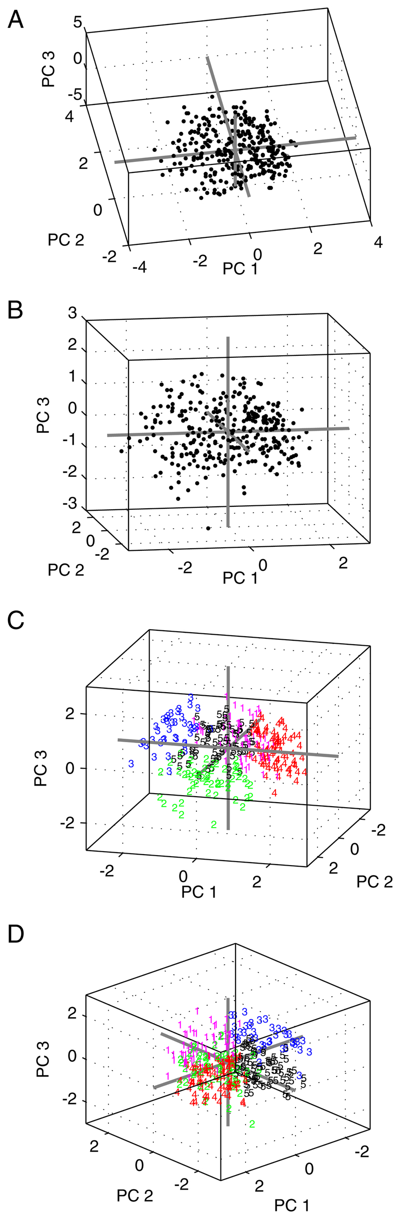
Three-dimensional scatterplots showing different views of the data distributed along the first 3 principal components. Gray lines are the axes of the eigenvectors intersecting at the origin. A and B: there is no suggestion that the data fall into discrete clusters. C and D: data have been partitioned into 5 clusters using k-means. Points are color-coded and numbered according to their designated cluster. Illustrative examples of the cluster members are shown in Figs. 12 and 13.

To test for the possibility that the distribution possesses modes in higher dimensions, we conducted a cluster validation analysis based on a validity index (Halkidi et al. 2001, 2002). We partitioned our data using k-means, an unsupervised iterative algorithm that picks out regions of compactness in a distribution by minimizing the distances between the data and k cluster centers. For each data point we calculated a so-called silhouette value, which is a cluster validity index. Silhouette values range from –1 to 1 and measure the strength of association between a unit and the cluster to which it has been attributed. Values ≳0.8 indicate that there is a strong association with the cluster, values close to zero indicate a lack of evidence for clustering, and negative values indicate that a data point may have been assigned to the wrong cluster. The mean of these silhouette values for all data points within one cluster is known as the “silhouette width” of that cluster and is a measure of both intercluster separation and intracluster compactness (Rousseeuw 1987).

We examined the mean silhouette widths (averaged over all clusters) for values of k between 2 and 30 (Fig. 11), running k-means 100 times for each value of k and choosing new random starting positions on each run. The algorithm was run for a maximum of 1,000 iterations during which it attempted to minimize the Euclidean distance between the data points and their assigned cluster center. The mean silhouette widths of our data barely exceeded 0.4 and became progressively smaller (indicating poorer cluster separability) as the data were partitioned into a larger number of putative binaural response classes. The silhouette width should peak when k equals the natural number of partitions (which might originate from isolated clusters or modes of a continuous distribution) in the data (Halkidi et al. 2002); the absence of such a peak for our data argues against the existence of such partitions. Nevertheless, the observed mean silhouette values are larger than those obtained by clustering normally distributed synthetic data (Fig. 11). This confirms what is seen in the 2D contour plots: that the distribution of binaural level functions exhibits a degree of structure and is not random or homogeneous. The low silhouette widths and absence of a peak at any k provide evidence that the distribution contains no distinct or partially overlapping response classes.

Fig. 11.

Mean silhouette widths (a measure of cluster separability) over all clusters. Values derived from k-means analysis as a function of cluster number (k). Results from the observed data (black) are compared with synthetic data (gray) consisting of a 5D Gaussian distribution with the same SDs as the observed data along each dimension. Silhouette widths of the observed data are calculated for 100 runs of k-means using randomly chosen starting points. For the synthetic data, 100 Gaussian distributions were created and silhouette widths obtained once for each. Error bars are drawn at 2 SD from the mean. Lack of a peak at any k suggests that no natural partitioning exists.

A data-driven analysis of response shape

Although the distribution of units in principal component space contains no structure that might indicate the presence of distinct binaural classes, the above analysis suggested that some response functions are more common than others. To investigate the degree to which the organization of our “shape space” relates to the classes of binaural interaction put forward in previous studies (e.g., Irvine et al. 1996; Rutkowski et al. 2000; Semple and Kitzes 1993a; Zhang et al. 2004), we first arbitrarily partitioned the data into five clusters and, second, explored properties of particular regions of the distribution.

partitioning of the response space

We partitioned the distribution into five clusters using the same k-means procedure described above. This is a simple way of seeing how different response functions are distributed in “shape space” and how those shapes are related to one another. We conducted this analysis for exploratory purposes only, not because the data naturally separate into five distinct classes. The preceding analysis provided no evidence that five-way partitioning is more appropriate than coarser or more fine grained subdivisions of the distribution.

The five-way partitioning of the data along the first three dimensions is illustrated in Fig. 10, C and D. Figures 12 and 13 show the shapes of the binaural response functions from each of these five arbitrary partitions. The positive skew along the first component occurs because most units fire maximally to sounds on the contralateral side: units with positive weightings along the first principal component (147/310 units) fall mainly into clusters 1 and 4 and have predominantly contralateral response shapes. The remaining units have negative weightings along the first component and fall largely into clusters 2, 3, and 5. Cluster 2 is composed of units exhibiting dual nonmonoto-nicity in ILD and ABL. Cluster 5 is similar, although these units have higher thresholds and so they exhibit a weaker nonmonotonicity in ABL. The units in these two clusters made up 41% (126/310 units) of our population. These binaural-level functions resemble the “TWIN” response type described by Semple and Kitzes (1993a,b), which they estimated to constitute 36% of their recorded units from cat primary auditory cortex (A1). The binaural response functions of the 20/53 units selected at random from cluster 2 (Fig. 13) resemble those in Semple and Kitzes (1993b) depicting representative examples of units with dual nonmonotonicity. Similarly, the major distinctions in the response shapes emerging from this analysis are like those picked out visually by Irvine et al. (1996). The responses in cluster 3 (39/310 units) are composed mostly of units with maximal responses on the ipsilateral side. This is in keeping with previous observations that few units are ipsi-dominant.

Fig. 12.

Five example responses from each of the 5 clusters into which the data were arbitrarily partitioned using k-means (see Figs. 12 and 13). Each row corresponds to a different cluster (cluster ID is indicated by the numbers along the left). Axes are the same as those in Fig. 3.

Fig. 13.

A–F: responses of units randomly selected from each of the 5 clusters into which the data were partitioned (see Fig. 10). Each plot superimposes the normalized responses from 20 units. Filled black regions represent the sound level combinations at which each unit fired at a ≥85% of its maximum response. Gray lines show the 75% contours for each unit. Colors of the 85% contours lines correspond to those in Figs. 10 and 14.

Despite the correspondence between our automated k = 5 analysis and the binaural interaction classes proposed by previous studies, our clustering validation analysis showed there to be no “natural” partitions in the distribution. The low silhouette values reported in the previous section indicate that alternative partitioning of the response space would be equally valid, implying that the boundaries between the five arbitrary clusters depicted in Fig. 10, C and D are not rooted in features of the distribution.

no significant modes in shape space

In this section we provide further support for the results of the clustering validation analysis by providing graphical evidence that the “shape space” contains no obvious modes that might be related to distinct binaural classes. We have shown that the data are not distributed homogeneously in principal component space in that some shapes occur more frequently than others. This inhomogeneity is seen most clearly along the first versus second, first versus fourth, and second versus fourth principal components, as illustrated in the scatter- and density plots in Fig. 14 (see also Fig. 9). Figure 14 shows three scatterplots (one for each pair of components) and associated 3D density plots. Data points are color-coded according to the cluster to which they were associated by the preceding k = 5 analysis. We have drawn boxes around areas of interest and labeled these with the Greek letters α to ζ. The binaural response functions of a random selection of 20 units in each box are shown below the density plots.

Fig. 14.

A–C: scatterplots showing the distribution of binaural response surfaces of the units against the 1st, 2nd, and 4th principal components (PC). These are the components along which most structure in the distribution is evident (also see Fig. 9). A: PC 1 vs. PC 2 shows 2 major peaks, α and β, which are indicated by the black boxes on the scatterplot. Colors of the data points show the cluster to which they were assigned by the k = 5, k-means analysis (Figs. 12 and 13). Labeled peaks, α and β, can also be seen in the 3D density plot below the scatterplot. Plots labeled α and β each show 20 units randomly selected from the corresponding boxed regions. Peak α contains mostly contralateral units, whereas peak β contains mostly midline-sensitive units. B: plot of PC 1 vs. PC 4 includes one region of high density, γ, containing units with contralateral maxima. δ is a region of very low density that contains mostly units with ipsilateral maxima. C: PC 2 vs. PC 4 is bimodal but the differences between peaks ε and ζ are not pronounced.

In all three cases the regions of highest density are associated with units that respond most strongly to contralateral ILDs. The most prominent peaks, α and γ, are composed of units from the contralaterally dominant clusters, 1 and 4 (the red and magenta points). Plotting a random selection of units from these peaks confirms this. Scatterplot C has the only compelling bimodality although both peaks, ε and ζ, are composed mainly of contralaterally dominant neurons. This bimodality therefore does not correspond to two subpopu-lations of cells with obviously different binaural response characteristics.

It has long been known that relatively few units in auditory cortex respond most strongly to sounds from the ipsilateral side. This is demonstrated in Fig. 14 through the very low density in the “ipsilateral region” of our shape space. Scatterplot B has only one region of high density, γ, and a region of low density, δ. Region δ is composed largely of ipsilaterally dominant units. Thus most points are from cluster 3 with some from clusters 2 and 5 (see Fig. 13). A similar organization is seen in scatterplot A.

The plots of the first versus second principal components (Fig. 14A) provide the only case where we see two peaks composed of units with different properties. The dominant peak, α, is contralateral, whereas peak β constitutes a small number of units with maxima near the 0 ILD axis. Although consistent with the possibility that midline units form a separate subpopulation in auditory cortex, many units from “mid-line clusters” 2 and 5 were not associated with this peak. Consequently, our data are more consistent with the view that there is a continuum, not composed of multiple modes, from contralateral to ipsilateral dominance. We make this suggestion by visually cross-referencing the color-coded points (Fig. 14) to the shapes of the clusters in Fig. 13.

Maximal responses and slopes

Measures such as Fisher information judge a response function to be most informative about the stimulus space at regions where the slope of the function is high (Dayan and Abbott 2001). Almost all units in clusters 1 and 4 had their regions of greatest response restricted to the contralateral side of the zero ILD axis, whereas units in clusters 2 and 5 exhibited maximal responses near to or on this axis. The tendency of neurons to restrict their responses to one side of or close to the zero ILD axis suggests that the maximum slopes should be elongated along and perpendicular to this axis.

Figure 15A shows the distribution over the binaural response surface of mean firing rates across all 310 units. The gray scale represents the number of times a particular level combination produced 90% of the maximum response over all units. To explore the dynamic coding range of the population, the magnitude of the gradient across each response function was calculated (functions were low-pass filtered before calculating the gradient), each was normalized by its maximum response, and the mean gradient over all cells was calculated (Fig. 15B). This simple analysis reveals two features in the data. First, the maximum slopes of the binaural level functions throughout the population lie along, and slightly ipsilateral to, the zero ILD axis. Second, this region of maximal slope is not parallel to zero ILD because it shifts further ipsilaterally with increasing sound level.

Fig. 15.

A: mean binaural response function over all 310 units. B: regions of greatest slope of the normalized response functions over the whole population. Each function was smoothed and normalized by the maximum response before calculation of the gradient. Gray scale indicates mean of the magnitude of the gradient at each point over all units. Region of greatest slope is elongated along the ABL axis, slightly ipsilateral to midline ILDs.

Discussion

Using PCA, a common multivariate statistical technique, we represented the binaural-level functions of units recorded from ferret auditory cortex in a metric space where the distribution was governed by the shape of the population’s response functions. We found that the data could be reliably modeled using the first five principal components. The distribution of the five-dimensional point cloud exhibited a degree of structure, but this is better thought of as a continuum rather than a small number of discrete or overlapping binaural response classes.

No evidence for discrete binaural classes

Our statistical approach is sufficiently robust to identify classes of binaural response shape should they exist. Modeling the data using the first five components adequately describes the underlying response shapes even if for some units the variance explained is low (Fig. 8). The cross-validation test (Fig. 6) shows that a five-dimensional space does not grossly underfit the data, thereby hiding clusters that might emerge only in higher-order models. We ran our analyses on models of ≤10 components (for which 70% of the variance is explained) and confirmed that this did not alter the results (data not shown).

The PCA created a five-dimensional “shape space” in which the Euclidean distance between points is inversely proportional to the similarity of their response functions. Our analysis of the inhomogeneity of the data point cloud (Figs. 12, 13, and 14) also acts as a control for our methodology, demonstrating that units close to each other in principal component space do indeed have similar response functions. Therefore if discrete classes of response shape exist, they ought to manifest themselves as isolated or partially overlapping regions of high density. Subjective visual inspection of the distribution (Figs. 9 and 10) and objective k-means clustering using a validity index (Fig. 11) provided no evidence for structure of this sort. This conclusion is also supported by plotting the results of the k = 5 partitioning (Figs. 12 and 13) and by examination of the peaks in the distribution (Fig. 14). We therefore conclude that there is a relatively featureless continuum of binaural-level functions in ferret auditory cortex.

There is no indication that the methods used for collecting the data could have biased our statistical analysis in a way that would compromise our conclusions. Most units (274/310) were recorded from the MEG, the location of the primary auditory cortical fields in the ferret (Bizley et al. 2005; Kowalski et al. 1995; Phillips et al. 1988), although some were located on the AEG where nonprimary fields have been identified (Bizley et al. 2005). We found no evidence that restricting our analysis to units from the MEG would change our conclusions. If the distribution of binaural response functions in auditory cortex arose from a small number of discrete or partially overlapping classes, these ought to be revealed by our analysis given the relatively large N in our study.

PCA and k-means are classical multivariate techniques commonly used for problems requiring unsupervised classification. We also applied other unsupervised approaches (data not shown) to this classification problem and obtained very similar results. These approaches included self-organizing maps, hierarchical clustering, Sammon mapping, and multidimensional scaling on the linear predictors of a generalized linear model.

Other studies also support a continuum

Previous studies of ILD sensitivity of cortical neurons at different ABLs have suggested that there might be a continuum from one-way to two-way nonmonotonicity (Semple and Kitzes 1993b) or from contralateral-dominant to ipsilateral-dominant responses (Irvine et al. 1996). However, this was difficult to establish explicitly because those studies did not represent the shapes of binaural level functions in a metric space. The approach used in the present study involved generating such a space, allowing us to explicitly confirm these suggestions (Fig. 14). Although we cannot rule out the possibility that classes of neurons with differential sensitivity to other binaural cues (i.e., interaural time differences or interau-ral spectral differences) might exist, a continuum of response properties is consistent with the range of spatial receptive fields of high-frequency A1 neurons reported in studies using either free-field (Imig et al. 1990; Rajan et al. 1990; Stecker et al. 2005) or virtual acoustic space (Mrsic-Flogel et al. 2005) stimulation. Recent findings indicate that this principle might also apply in visual cortex by showing that simple and complex cells—a classic dichotomy—are likely to form a continuous distribution rather than discrete response types (Bair 2005; Mechler and Ringach 2002; Rust et al. 2005).

Relationship to previous classification studies

Our study is fundamentally different from previous work in which binaural properties were classified with respect to monaural responses. We did not include responses to monaural stimulation because they are not required to quantify the shapes of the binaural response functions. It is therefore not possible to make a direct comparison between the results of our approach and those from traditional classification schemes. However, in this section we argue that, for more extensive binaural stimulus sets, multivariate techniques based on response shape are more appropriate and useful than traditional classification schemes.

In early studies of auditory cortex (e.g., Imig and Adrian 1977), binaural interactions were defined by comparing binau-ral responses at a single reference sound level to those evoked by monaural stimulation of each ear. This approach provided a convenient and unambiguous scheme for data reduction with these simple stimuli. However, it is less applicable to more complex stimulus sets. Some recent studies have partitioned binaural interactions into as many as 14 different classes (Rutkowski et al. 2000; Zhang et al. 2004). These classification schemes are useful for defining the nature of the monaural inputs and their interactions within auditory cortex. However, these schemes are confusing because they contain a large number of classes that, being nominal variables, are not linked by a scale and so their relationship is not clear-cut. Furthermore, the lack of a scale means that there is no way of measuring intra- or interclass similarity, and thus the separability of the putative binaural classes cannot be determined. Because these studies have, on average, only 10 to 20 neurons per class (Rutkowski et al. 2000; Zhang et al. 2004) it seems likely that they arbitrarily partition a continuum of binaural response properties. For these reasons, a data reduction approach that does not rely on drawing arbitrary class boundaries is more appropriate. We suggest that our approach provides a more useful description of the data than traditional classification schemes. By using PCA to describe the shape-related variance of a population of neurons, we can quantify the features of the responses most relevant to the coding of the stimulus space. Because this is done in a metric space of ratio variables, we can measure the similarity between the binaural responses of these neurons.

Classification schemes in mapping studies

Early recording studies reported that the binaural organization of A1 in the anesthetized cat, the most extensively studied species, is columnar. Neurons within a column that runs orthogonal to the cortical surface were found to have the same binaural response properties (Abeles and Goldstein 1970; Imig and Adrian 1977). Later reports described bands of cells with similar binaural properties elongated approximately orthogonal to the isofrequency axis (Middlebrooks et al. 1980). Such bands have also been found in the cat’s secondary auditory cortical area (Schreiner and Cynader 1984). Subsequent physiological investigations, in which more extensive classification schemes have been used, have failed to confirm the existence of these binaural bands. Instead, it appears that neurons with similar binaural properties are arranged in circumscribed clusters (or patches) across the cortical surface. This type of organization has been reported in anesthetized ferrets (Kelly and Judge 1994; Phillips et al. 1988), albino rats (Kelly and Sally 1988), guinea pigs (Rutkowski et al. 2000), cats (Nakamoto 2004; Reale and Kettner 1986), and owl monkeys (Recanzone et al. 1999). The relatively recent discovery of binaural clusters reflects the way the data have been classified. The studies that have found evidence for binaural clusters within the cortex are generally those based on more extensive stimulus sets and therefore more complex, fine-grained, binau-ral classification schemes (Nakamoto et al. 2004; Reale and Kettner 1986; Rutkowski et al. 2000).

It is difficult to avoid the conclusion that the apparent distribution of binaural properties depends on the complexity of the classification schemes used. Coarser binaural classification schemes of the type originally used will produce larger clusters across the cortical surface as they group neurons with more disparate properties. Although neighboring neurons generally do have similar response properties (but see Linden and Schreiner 2003 for a review of interlaminar variations that have been described in auditory cortex), we suggest that the boundaries and sizes of the proposed clusters (e.g., Nakamoto et al. 2004; Rutkowski et al. 2000) should be viewed with caution. The similarity between putative binaural response classes has not previously been measured, and so there was no way of quantifying the differences between neighboring patches of cortical neurons based on their binaural interactions. Because PCA does not arbitrarily partition the data, the similarity between binaural response functions recorded in different regions of the auditory cortex can be measured. Our approach could therefore be readily extended to cortical mapping studies by projecting electrode location or depth onto the “shape space.”

Functional significance of a continuum

A continuum of response properties is what might be expected if even sampling of the stimulus space is to be achieved within the neuronal population. From a coding perspective, nonoverlapping clusters would be surprising because stimuli falling between the clusters would not be well represented. As indicated earlier, some response types are more common than others in auditory cortex so the stimulus space is not evenly sampled. Figure 15 shows that over the whole population of units, the region of greatest slope occurs within the physiological range and particularly at small ILD values. The distribution of ILD responses of cortical neurons therefore appears to be optimized for representing the naturally experienced range of ILDs. A similar result has been found in the guinea pig inferior colliculus where low-frequency neurons tend to respond best to interaural timing differences outside the physiological range. This means that the maximum slope (McAlpine et al. 2001) and therefore the maximum Fisher information (Harper and McAlpine 2004) occur within that range. In the free field, this also accords with the slopes of the azimuth response functions recorded in different cortical fields of the cat by Stecker et al. (2005). Because behavioral acuity is greatest near the midline (e.g., Mills 1958; Parsons et al. 1999), these studies suggest that the maximum spatial information is conveyed by the slope rather than the peak of the response functions. Nevertheless, our analysis shows that, within the same hemisphere, binaural-level functions vary along a continuum from those exhibiting sensitivity to ipsilateral sound locations to the majority that prefer contralateral stimulation.

References

- Abeles M, Goldstein MH., Jr Functional architecture in cat primary auditory cortex: columnar organization and organization according to depth. J Neurophysiol. 1970;33:172–187. doi: 10.1152/jn.1970.33.1.172. [DOI] [PubMed] [Google Scholar]
- Bair W. Visual receptive field organization. Curr Opin Neurobiol. 2005;15:459–464. doi: 10.1016/j.conb.2005.07.006. [DOI] [PubMed] [Google Scholar]
- Bajo VM, Nodal FR, Bizley JK, Moore DR, King AJ. The ferret auditory cortex: descending projections to the inferior colliculus. Cereb Cortex. 2006 Mar 31; doi: 10.1093/cercor/bhj164. Epub ahead of print. [DOI] [PMC free article] [PubMed] [Google Scholar]
- Bizley JK, Nodal FR, Nelken I, King AJ. Functional organization of ferret auditory cortex. Cereb Cortex. 2005;15:1637–1653. doi: 10.1093/cercor/bhi042. [DOI] [PubMed] [Google Scholar]
- Dayan P, Abbott LF. Cambridge, MA: MIT Press; 2001. Theoretical Neuroscience: Computational and Mathematical Modeling of Neural Systems. [Google Scholar]
- Duda RO, Martens WL. Range dependence of the response of a spherical head model. J Acoust Soc Am. 1998;104:3048–3058. [Google Scholar]
- Halkidi M, Batistakis Y, Vazirgiannis M. On clustering validation techniques. J Intell Inf Syst. 2001;17:107–145. [Google Scholar]
- Halkidi M, Batistakis Y, Vazirgiannis M. ACM SIGMOD Record. Vol. 31. New York: Association for Computing Machinery, Online; 2002. Clustering validity checking methods: Part II; pp. 19–27. May be accessed at usacm@acm.org. [Google Scholar]
- Harper NS, McAlpine D. Optimal neural population coding of an auditory spatial cue. Nature. 2004;430:682–686. doi: 10.1038/nature02768. [DOI] [PubMed] [Google Scholar]
- Heffner HE, Heffner RS. Effect of bilateral auditory cortex lesions on sound localization in Japanese macaques. J Neurophysiol. 1990;64:915–931. doi: 10.1152/jn.1990.64.3.915. [DOI] [PubMed] [Google Scholar]
- Imig TJ, Adrian HO. Binaural columns in the primary field (A1) of cat auditory cortex. Brain Res. 1977;138:241–257. doi: 10.1016/0006-8993(77)90743-0. [DOI] [PubMed] [Google Scholar]
- Imig TJ, Irons WA, Samson FR. Single-unit selectivity to azimuthal direction and sound pressure level of noise bursts in cat high-frequency primary auditory cortex. J Neurophysiol. 1990;63:1448–1466. doi: 10.1152/jn.1990.63.6.1448. [DOI] [PubMed] [Google Scholar]
- Irvine DRF. A comparison of two methods for the measurement of neural sensitivity to interaural intensity differences. Hear Res. 1987;30:169–179. doi: 10.1016/0378-5955(87)90134-1. [DOI] [PubMed] [Google Scholar]
- Irvine DRF, Rajan R, Aitkin LM. Sensitivity to interaural intensity differences of neurons in primary auditory cortex of the cat. I. Types of sensitivity and effects of variations in sound pressure level. J Neurophysiol. 1996;75:75–96. doi: 10.1152/jn.1996.75.1.75. [DOI] [PubMed] [Google Scholar]
- Kavanagh GL, Kelly JB. Contribution of auditory cortex to sound localization by the ferret (Mustela putorius) J Neurophysiol. 1987;57:1746–1766. doi: 10.1152/jn.1987.57.6.1746. [DOI] [PubMed] [Google Scholar]
- Kelly JB, Judge PW. Binaural organization of primary auditory cortex in the ferret (Mustela putorius) J Neurophysiol. 1994;71:904–913. doi: 10.1152/jn.1994.71.3.904. [DOI] [PubMed] [Google Scholar]
- Kelly JB, Sally SL. Organization of auditory cortex in the albino rat: binaural response properties. J Neurophysiol. 1988;59:1756–1769. doi: 10.1152/jn.1988.59.6.1756. [DOI] [PubMed] [Google Scholar]
- Kowalski N, Versnel H, Shamma SA. Comparison of responses in the anterior and primary auditory fields of the ferret cortex. J Neurophysiol. 1995;73:1513–1523. doi: 10.1152/jn.1995.73.4.1513. [DOI] [PubMed] [Google Scholar]
- Linden JF, Schreiner CE. Columnar transformations in auditory cortex? A comparison to visual and somatosensory cortices. Cereb Cortex. 2003;13:83–89. doi: 10.1093/cercor/13.1.83. [DOI] [PubMed] [Google Scholar]
- Machens CK, Wehr MS, Zador AM. Linearity of cortical receptive fields measured with natural sounds. Neuroscience. 2004;24:1089–1100. doi: 10.1523/JNEUROSCI.4445-03.2004. [DOI] [PMC free article] [PubMed] [Google Scholar]
- Malhotra S, Hall AJ, Lomber SG. Cortical control of sound localization in the cat: unilateral cooling deactivation of 19 cerebral areas. J Neuro-physiol. 2004;92:1625–1643. doi: 10.1152/jn.01205.2003. [DOI] [PubMed] [Google Scholar]
- McAlpine D, Jiang D, Palmer AR. A neural code for low-frequency sound localization in mammals. Nat Neurosci. 2001;4:396–401. doi: 10.1038/86049. [DOI] [PubMed] [Google Scholar]
- Mechler F, Ringach DL. On the classification of simple and complex cells. Vision Res. 2002;42:1017–1033. doi: 10.1016/s0042-6989(02)00025-1. [DOI] [PubMed] [Google Scholar]
- Middlebrooks JC, Dykes RW, Merzenich MM. Binaural response-specific bands in primary auditory cortex (AI) of the cat: topographical organization orthogonal to isofrequency contours. Brain Res. 1980;181:31–48. doi: 10.1016/0006-8993(80)91257-3. [DOI] [PubMed] [Google Scholar]
- Mills AW. On the minimum audible angle. J Acoust Soc Am. 1958;30:237–246. [Google Scholar]
- Mrsic-Flogel TD, King AJ, Schnupp JWH. Encoding of virtual acoustic space stimuli by neurons in ferret primary auditory cortex. J Neurophysiol. 2005;93:3489–3503. doi: 10.1152/jn.00748.2004. [DOI] [PubMed] [Google Scholar]
- Nakamoto KT, Zhang J, Kitzes LM. Response patterns along an isofrequency contour in cat primary auditory cortex (AI) to stimuli varying in average and interaural levels. J Neurophysiol. 2004;91:118–135. doi: 10.1152/jn.00171.2003. [DOI] [PubMed] [Google Scholar]
- Parsons CH, Lanyon RG, Schnupp JWH, King AJ. Effects of altering spectral cues in infancy on horizontal and vertical sound localization by adult ferrets. J Neurophysiol. 1999;82:2294–2309. doi: 10.1152/jn.1999.82.5.2294. [DOI] [PubMed] [Google Scholar]
- Phillips DP, Irvine DRF. Some features of binaural input to single neurons in physiologically defined area AI of cat cerebral cortex. J Neuro-physiol. 1983;49:383–395. doi: 10.1152/jn.1983.49.2.383. [DOI] [PubMed] [Google Scholar]
- Phillips DP, Judge PW, Kelly JB. Primary auditory cortex in the ferret (Mustela putorius): neural response properties and topographic organization. Brain Res. 1988;443:281–294. doi: 10.1016/0006-8993(88)91622-8. [DOI] [PubMed] [Google Scholar]
- Rajan R, Aitkin LM, Irvine D. Azimuthal sensitivity of neurons in primary auditory cortex of cats. I. Types of sensitivity and the effects of variations in stimulus parameters. J Neurophysiol. 1990;64:872–887. doi: 10.1152/jn.1990.64.3.872. [DOI] [PubMed] [Google Scholar]
- Reale RA, Kettner RE. Topography of binaural organization in primary auditory cortex of the cat: effects of changing interaural intensity. J Neu-rophysiol. 1986:663–682. doi: 10.1152/jn.1986.56.3.663. [DOI] [PubMed] [Google Scholar]
- Recanzone GH, Schreiner CE, Sutter ML, Beitel RE, Merzenich MM. Functional organization of spectral receptive fields in the primary auditory cortex of the owl monkey. J Comp Neurol. 1999;415:460–481. doi: 10.1002/(sici)1096-9861(19991227)415:4<460::aid-cne4>3.0.co;2-f. [DOI] [PubMed] [Google Scholar]
- Rousseeuw PJ. Silhouettes: a graphical aid to the interpretation and validation of cluster analysis. J Comp Appl Math. 1987;20:53–65. [Google Scholar]
- Rust NC, Schwartz O, Movshon JA, Simoncelli EP. Spatiotemporal elements of macaque V1 receptive fields. Neuron. 2005;46:945–956. doi: 10.1016/j.neuron.2005.05.021. [DOI] [PubMed] [Google Scholar]
- Rutkowski RG, Wallace MN, Shackleton TM, Palmer AR. Organisation of binaural interactions in the primary and dorsocaudal fields of the guinea pig auditory cortex. Hear Res. 2000;145:177–189. doi: 10.1016/s0378-5955(00)00087-3. [DOI] [PubMed] [Google Scholar]
- Sahani M, Linden JF. How linear are auditory cortical responses? In: Becker S, Thrun S, Obermayer K, editors. Advances in Neural Information Processing Systems. Vol. 15. Cambridge, MA: MIT Press; 2003. pp. 109–116. [Google Scholar]
- Schreiner CE, Cynader MS. Basic functional organization of second auditory cortical field (AII) of the cat. J Neurophysiol. 1984;51:1284–1305. doi: 10.1152/jn.1984.51.6.1284. [DOI] [PubMed] [Google Scholar]
- Semple MN, Kitzes LM. Binaural processing of sound pressure level in cat primary auditory cortex: evidence for a representation based on absolute levels rather than interaural level differences. J Neurophysiol. 1993a;69:449–461. doi: 10.1152/jn.1993.69.2.449. [DOI] [PubMed] [Google Scholar]
- Semple MN, Kitzes LM. Focal selectivity for binaural sound pressure level in cat primary auditory cortex: two-way intensity network tuning. J Neurophysiol. 1993b;69:462–473. doi: 10.1152/jn.1993.69.2.462. [DOI] [PubMed] [Google Scholar]
- Smith AL, Parsons CH, Lanyon RG, Bizley JK, Akerman CJ, Baker GE, Dempster AC, Thompson ID, King AJ. An investigation of the role of auditory cortex in sound localization using muscimol-releasing Elvax. Eur J Neurosci. 2004;19:3059–3072. doi: 10.1111/j.0953-816X.2004.03379.x. [DOI] [PubMed] [Google Scholar]
- Stecker GC, Harrington IA, Middlebrooks JC. Location coding by opponent neural populations in the auditory cortex. PLoS Biol. 2005;3:e78. doi: 10.1371/journal.pbio.0030078. [DOI] [PMC free article] [PubMed] [Google Scholar]
- Zhang J, Nakamoto KT, Kitzes LM. Binaural interaction revisited in the cat primary auditory cortex. J Neurophysiol. 2004;91:101–117. doi: 10.1152/jn.00166.2003. [DOI] [PubMed] [Google Scholar]