

Abstract
SARS struck Taiwan in 2003, causing a national crisis. Many people feared that SARS would spread through the health care system, and outpatient visits fell by more than 30% in the course of a few weeks. We examine how both public information and the behavior and opinions of peers contributed to this reaction. We identify a peer effect through a difference-in-difference comparison of longtime residents and recent arrivals, who are less socially connected. Although several forms of social interaction may contribute to this pattern, social learning is a plausible explanation for our finding. We find that people respond to both public information and to their peers. In a dynamic simulation based on the regressions, social interactions substantially magnify the response to SARS.
Keywords: SARS, Social learning, Peer effects, Prevalence response, Economic epidemiology, Crisis
Highlights
-
•
We assess how peer effects contributed to the response to SARS in Taiwan.
-
•
We compare long-time residents and recent arrivals, who are less socially connected.
-
•
Social learning is a plausible reason why peer effects increase during this period.
-
•
Social interactions contributed to the fall in health care utilization during SARS.
1. Introduction
The public periodically confronts a novel and unfamiliar threat, such as a terrorist attack or new disease outbreak. These situations typically spur people to take extreme protective actions such as avoiding public places, putting down livestock, or curtailing air travel. In a crisis, a person must assess a new risk and decide how aggressively to protect himself. However, it is unclear how people make these decisions given the scarcity of information about the severity or prevalence of the threat.
The 2003 SARS epidemic in Taiwan allows us to study the response to an unfamiliar risk. SARS (severe acute respiratory syndrome) is a respiratory illness that resembles severe pneumonia and is transmitted through close interpersonal contact. SARS reached Taiwan from mainland China in March of 2003. 312 people were confirmed to be infected and 82 people died before the epidemic disappeared in July of that year. Despite the low prevalence of SARS in the general population, the public strongly eschewed restaurants, shopping centers, and other public places (Chou et al., 2004, Siu and Wong, 2004). The high infection rate in hospitals also caused people to avoid the health care system: outpatient visits fell by 31% in April and May of 2003 (Hsieh et al., 2004). This drop occurred both in locations with and without SARS, and persisted for months after the epidemic had passed.
Health care avoidance during SARS is an example of a “prevalence response” which is a familiar topic in the literature on economic epidemiology (Ahituv et al., 1996, Gersovitz and Hammer, 2003, Lakdawalla et al., 2006). Facing an increase in disease risk, people protect themselves and thereby limit the spread of infection. With few exceptions (de Paula et al., 2011, Gong, forthcoming), this literature has assumed that decision makers possess complete information, which is an unrealistic assumption in a disease outbreak. In even the most saturated media environment, public announcements only weakly indicate a person's idiosyncratic infection risk. Without a precise public signal, people may rely on private signals such as the opinions and actions of their peers. This mechanism may cause an “information cascade” that magnifies the response to an unfamiliar threat (Banerjee, 1992, Bikchandani et al., 1992, Welch, 1992). If social learning is an important determinant of behavior in this setting, it may determine the effectiveness of public policies to address a crisis.
This paper measures the contributions of public risk information and signals from peers to the SARS response. Reports of local and national SARS incidence provide public risk signals. We proxy for the risk signal of peers using the change in health care utilization among peers from a pre-SARS baseline, which derives from a simple model of health care demand. A regression of individual medical visits on these variables distinguishes between the contributions of public information and peer signals. Our analysis uses a nationally representative panel of medical claims of 1 million people (4.3% of Taiwan's population). This source allows us to quantify the number of outpatient visits by patient, provider and two-week period from 2001 to 2003 for a 16% subsample of this data set. We proxy for peer groups, which the claims data do not directly measure, using cohorts of patients who visit a common physician and facility.
Identifying a peer effect through a regression of individual outcomes on group outcomes is challenging because common unobservables jointly determine both variables (Manski, 2000). Patients may sort into peer groups because of common risk or health preferences. Heterogeneous supply shocks, such as office closures by some doctors, may also induce a spurious correlation. Patients in the same peer group may receive correlated signals of SARS risk if they obtain news from the same media sources. We address these concerns through a difference-in-difference design that compares the response of longtime community residents (“non-movers”) to the response of recent arrivals (“movers”). Although these groups face a similar (vanishingly small) risk of contracting SARS, non-movers have stronger social ties to their communities. We find that non-movers respond more to their peers than to local SARS incidence but less than to national SARS incidence. This identification strategy places a lower bound on the peer effect because it is based on a differential response.
Our identifying assumption is that unobservable shocks to visits do not differentially affect non-movers during the SARS period. We evaluate this assumption through a complementary approach in which we address common unobservables by controlling for current peer visits. This strategy relies on variation in lagged peer visits for identification. Fixing current visits, a peer group whose visits were previously high conveys a stronger signal of SARS risk than a group whose visits were previously low. By specifically controlling for the visits of non-mover peers, we deal with the concern that shocks specific to non-movers confound the difference-in-difference regressions. In a final falsification test, we apply our methodology to the annual drop in visits that occurs during Chinese New Year and find that peer effects do not explain this phenomenon.
Social learning is a plausible channel through which social interactions increased during SARS. The severity of SARS creates a demand for information about SARS risk. Information is scarce during a novel epidemic, as even experts lack basic facts about the disease. In the absence of more reliable signals, people may learn from the behaviors and perceptions of their peers. Several mechanisms other than social learning may contribute to our peer effect estimate. In principle, SARS contagion among peers may cause a positive correlation in peer visits during the SARS period. This mechanism is not a serious confound in practice because SARS prevalence is very low, even in the highest-risk townships.1 Alternatively, people may imitate rather than learn from their peers. We cannot distinguish learning from imitation without richer data. Finally, the visits of peers may be negatively correlated through congestion at health care facilities, which also causes our estimates to be a lower bound.
This paper contributes to the literature on economic epidemiology by analyzing the “prevalence response” to disease risk. We consider the context of health care utilization, which is intrinsically interesting because it directly affects health (e.g. Card et al., 2009, Currie and Gruber, 1996). To date, this literature has focused on HIV and has identified responses to both public and private signals (de Paula et al., 2011, Delavande and Kohler, 2012, Philipson and Posner, 1995, Thornton, 2008). Our study complements these papers by providing the first assessment of how peer effects influence the response to disease risk.
The paper also contributes to the literature on social learning. Studies have demonstrated social learning in the context of technology adoption and consumption (e.g. Conley and Udry, 2010, Foster and Rosenzweig, 1995, Moretti, 2011, Munshi, 2004). Studies of learning and medical utilization (Deri, 2005, Oster and Thornton, 2011) consider day-to-day decisions rather than behavior during a medical crisis. Because of the dearth of objective information during an emergency, the nature and magnitude of social learning may be different than under ordinary circumstances. Randomization is not available as a tool to study social interactions during a crisis. We build upon attempts to identify peer effects in observational data by defining a subset of people who are less exposed to peers. As with other non-experimental peer effect studies, it is difficult to rule out omitted variable bias definitively.
Finally, the paper contributes to the literature on crisis response. A key question is why negligible changes in objective risk substantially alter individual choices. For instance, objectively small terrorism and health risks have large impacts on commerce (Abadie and Gardeazabal, 2003, Blunk et al., 2006, Kraipornsak, 2010). Becker and Rubinstein (2011) find that Israeli tourists respond more strongly to terrorism risk than local residents, and suggest that people who regularly confront risk may invest in the ability to surmount an emotional response. Social interactions may also explain why people adopt mistaken beliefs and respond in extreme ways to a crisis. The magnitude of this private response determines the impact of a crisis. Just as air travel reductions after 9/11 caused more people to die in traffic accidents than in the attacks themselves (Blalock et al., 2009), health care avoidance during SARS may have caused more deaths than the epidemic itself.2
We proceed in Section 2 to motivate and justify our empirical approach. This section shows the assumptions under which our empirical strategy identifies a peer effect. Section 3 describes the health care setting in Taiwan, the SARS epidemic, and the data set. Regression results appear in Section 4. Section 5 describes a dynamic simulation of the aggregate response to SARS. Section 6 discusses the interpretation of our findings and Section 7 concludes.
2. Empirical overview
In this section, we offer a theoretical motivation for our empirical approach. We regress the change in individual visits on the change in peer visits and use a difference-in-difference strategy to disentangle social interactions from common unobservables. As an alternative, we regress the change in individual visits separately on current and lagged peer visits. First we explain why the change in visits is a valid proxy for subjective SARS risk. Next we specify the identifying assumptions of these strategies. In Appendix A, a full model of belief formation derives the relationship between the regression coefficients and the structural parameters of a social learning model.
2.1. The change in visits as a proxy for subjective SARS risk
Our analysis focuses on an individual's subjective assessment of the risk of SARS death during a medical visit, s ijt ∈ [0, 1], which is indexed by individual i, peer group j, and time period t. We proxy for sijt, which is unobservable, with the change in an individual's medical visits compared to a period before the SARS epidemic when sijt = 0. To motivate this proxy, suppose a person has health care demand vijt = αi − δpijt. In this equation, vijt ≥ 0 and pijt are the patient's quantity and out-of-pocket price of care, while δ ≥ 0 and αi ≥ 0 are the slope and individual-specific intercept of the demand curve. Fig. 1 represents the equilibrium in the health care market.
Fig. 1.

Inference about SARS risk from a change in visits.
Like a tax, SARS risk increases the perceived cost of health care. Let the multiplier π > 0 convert SARS risk into a monetary value. The figure illustrates how SARS shifts the out-of-pocket price upward to pijt + πsijt, moving along the demand curve. Because the demand curve provides a one-to-one mapping between quantity and price, the difference in quantity yields the monetary value of SARS risk: ∆vijt = vijt − v ijt − 1 = δπsijt. An observer with knowledge of δ and π can perfectly derive SARS risk from a change in visits if supply remains constant. The signal is weaker but still informative if the observer must estimate the demand parameters. In practice, the change in peer visits is consistent with information transmission from various sources, including direct observation and communication from doctors or peers.
2.2. Identification of a peer effect
Below we regress the change in individual visits on a common signal of risk, s jt c, and the change in peer visits . Two factors may confound this regression. First, common unobservables may jointly influence individual and group behavior, causing a spurious correlation between vijt and (Manski, 1993, Manski, 2000). Heterogeneous supply shocks such as office closures by some doctors may cause a correlation in the visits of patients of the same doctor. Patients and their peers, having self-selected into the same group, may also share common traits such as risk aversion. Group members may receive common risk signals. In a second threat to identification, people may receive unobservable private risk signals, s ijt p, which reflect their idiosyncratic risk preferences or Bayesian prior beliefs.
The following hypothetical regression incorporates these factors.
| (1) |
In this equation, λ 1 and λ 2 are the weights people place on the common signal and the peer signal. λ 3 captures the potential spurious correlation between vijt and , and λ 4 is the weight people place on the private signal. In principle, λ 1, λ 2, and λ 4 must sum to 1 if they exhaust all possible learning channels. Because of this constraint, information sources are substitutable.
We implement a difference-in-difference regression that compares non-movers, who are long-time neighborhood residents, with movers, who have recently joined the community and peer group. We examine the correlation between individual and group outcomes for each type of person before and during the SARS epidemic. Our identifying assumption is that unobservable shocks to visits do not differentially affect non-movers during the SARS period. To examine this strategy, we decompose each coefficient, λr, into type-specific and period-specific elements: λ r = λ r θ + λ r τ + λ r θτ, for r ∈ {1, 2, 3, 4}. θ ∈ {m, n} denotes the person type (mover or non-mover), and τ ∈ {p, d} denotes the period (prior to SARS or during SARS).
Equivalently, we express this decomposition using dummy variables for the non-movers and the SARS period, Ni and Dt: λ j = λ j mp + (λ j np − λ j mp)N i + (λ j md − λ j mp)D t + (λ j nd − λ j md)N i D t. Next we substitute this expression into Eq. (1), noting that s jt c and s ijt p equal zero prior to SARS.
| (2) |
In this expression, Ωijt denotes the level effect of and its pairwise interactions with Ni and Dt.3 The private signal, which is unobservable, appears in the error term: ξ ijt = λ 4 md D t s ijt p + [λ 4 nd − λ 4 md] N i D t s ijt p + ε ijt. Our empirical objective is to identify λ 1 md, λ 1 nd, and [λ 2 nd − λ 2 md].
The primary identifying assumption of this regression is that common unobservables have the same effect on movers and non-movers during the SARS period: λ 3 md = λ 3 nd. Under this assumption, the differential effect of common unobservables during SARS cancels and the coefficient for isolates a peer effect. This regression controls for any shock that is common to movers and non-movers, including supply heterogeneity. Our approach provides a lower bound estimate of the peer effect because it excludes any social interactions by movers during SARS as well as social interactions by either group prior to SARS (λ 2 mp, λ 2 np and λ 2 md).
We provide further evidence using a complementary identification strategy that does not distinguish between movers and non-movers. Instead we regress the change in individual visits on current and one-year lagged peer visits with a SARS period interaction. Common unobservables primarily threaten identification by causing a correlation between contemporaneous values of vijt and . However Fig. 1 illustrates that lagged visits also contain information about a person's risk perception. Fixing current visits, a peer group with previously high utilization provides a larger risk signal than a peer group with previously low utilization. Contemporaneous shocks are unlikely to confound the differential effect of lagged peer visits during SARS, since these visits occur prior to the epidemic.
We implement this approach by regressing the change in individual visits on current and one-year lagged peer visits with a SARS period interaction. The identifying assumption is that while common unobservables may confound the effect of , they do not confound the effect of differentially during SARS. In the following specification, λ denotes a contemporaneous effect and denotes an effect with a one-year lag.
| (3) |
In this expression, Φijt contains the uninteracted effects of and .4 As above, the private signal appears in the error term: ν ijt = λ 4 d D t s ijt p + ε ijt. To identify a social interaction, we must assume that . Due to the one-year lag, is always measured prior to SARS. To confound this estimate, common unobservables must cause a greater correlation between these variables in 2002 than in 2001.
In this regression, controls for unobservable shocks during the SARS period. By separately controlling for of movers and non-movers (and interacting these variables with Ni), we can directly control for type-specific unobservable shocks. These shocks are the remaining threat to identification under the difference-in-difference approach above. By examining the sensitivity of our estimates to these controls, we can test the validity of the main identifying assumption of the difference-in-difference approach.
Unobservable private signals may also threaten identification. A second identifying assumption that applies to both approaches is that the difference between the private signals of any two group members must be orthogonal to the regressors: and . This assumption assures that the regressors are uncorrelated with ξijt, which is plausible if individual private signals are independent draws from a common distribution within the group.5
3. Context and data
3.1. The SARS epidemic in Taiwan
Taiwan is a densely populated island located near mainland China. The country has a population of 23.1 million and income per capita of around $31,000. Modern highways and railways facilitate intercity travel. Taiwan is made up of 25 counties and cities, which further subdivide into 368 townships and urban districts (hereafter labeled “counties” and “townships” respectively). The population has a median age of 37 and a life expectancy of 78. Chinese New Year, which occurs on a lunar schedule in January or February, is an important holiday that causes a large decline in medical visits. During the two-week holiday, many families travel to visit relatives and some medical offices are closed. This holiday has a large impact on health care utilization in the figures below.
In 1996, Taiwan implemented a universal fee-for-service health care system (Cheng, 2003). Under the system, patients contribute modest copayments of US$5 or less for visits, tests, and prescriptions. The Bureau of National Health Insurance (BNHI) administers the system and reimburses providers for most expenses. People may obtain outpatient care from either hospital outpatient departments or small storefront clinics. Clinics, which are ubiquitous in cities, serve around 70% of the outpatient market. With such low copayments, many patients prefer to visit the doctor (and obtain medicine) for minor illnesses such as sore throats and colds. These conditions, classified broadly as “upper respiratory infections” constitute 38% of all outpatient visits. The low out-of-pocket cost has led to intense health care utilization, with patients seeking care a median of 10 times per year.
SARS is a respiratory illness that resembles severe pneumonia. The disease is caused by a coronavirus and is transmitted through close contact with an infected person. The SARS epidemic originated in Guangdong, China in November of 2002 and soon spread to Hong Kong, Southeast Asia, and Canada. Taiwan's first SARS case occurred in a traveler who became ill on March 14, 2003 after arriving from mainland China. The epidemic escalated on April 22 when an indigenous outbreak among patients and hospital staff at the Ho-Ping Hospital in Taipei led to several secondary outbreaks in other major cities. Fig. 2 plots the number of reported and probable SARS cases (explained below) by two-week period to show the progression of the epidemic. The SARS epidemic lasted through June, leading to a total of 312 confirmed infections and 82 deaths. At the peak of the epidemic, SARS infected 60 and killed 6 people per day. Nevertheless, the overall burden of SARS was only 1.4 confirmed cases and 0.36 deaths per 100,000 people.
Fig. 2.

SARS cases by two-week period during 2003.
The Ho-Ping Outbreak, which took place during Period 9 in the figure, led to widespread panic. According to Ko et al. (2006, p. 398), “People started to hoard all possible protective equipment, and reject people or materials with any risk of infection, including infected patients, the families of patients, subjects quarantined, and even health providers.” Domestic air travel fell by 30% and international air travel fell by 58% from 2002 levels (National Policy Foundation, 2003). The price of Isatidis Radix, a traditional Chinese antiviral remedy, rose by 800% (Huang, 2003).
The SARS epidemic also had a large impact on health care utilization. Fig. 3 plots the nationwide volume of outpatient visits by two-week period in 2001, 2002, and 2003. In a sharp deviation from the usual seasonal pattern, visits fell by over 30% from March to June of 2003. Visits did not return to the pre-SARS level until September of that year, three months after the last probable SARS case on June 16. Based on the number of SARS deaths and outpatient visits from March to June of 2003, SARS created a mortality risk of at most 0.0000007 deaths per visit. Using an upper-bound estimate of $2.2 million for the value of statistical life (Hammitt and Liu, 2004), the risk of SARS death during a medical visit raised the expected price of a visit by $1.93. However the decline in visits during SARS is consistent with a much larger perceived cost. After a copayment increase of $3 in November of 2002, visits to medical centers fell by 3%. Benchmarking the SARS response by this copayment response, people behaved as if SARS had increased the price of a visit by $17.60.6
Fig. 3.

Aggregate outpatient visits by two-week period: 2001–2003.
The response to SARS occurred both in townships with and without actual SARS incidence. Fig. 4 plots total visits, comparing townships with zero and positive SARS incidence. The response to SARS is only slightly larger in townships that actually experienced the outbreak. The timing and magnitude of the SARS response also depended on the nature of the visit. Fig. 5 categorizes visits as respiratory, critical, chronic, or other.7 Although utilization fell in all categories, the response of respiratory visits was particularly sharp and extended. These visits fell by over 50% and remained suppressed through the end of the year. Although respiratory visits are distinct in several aspects, the low marginal benefit of a respiratory visit is the most likely explanation for this pattern.8
Fig. 4.

Visits for SARS-affected and -unaffected townships during 2003.
Fig. 5.

Visits by diagnosis during 2003.
3.2. Data
Our primary data source is a large panel of medical claims furnished by the BNHI. The data set contains all outpatient visits from 1997 to 2003 for a representative sample of one million people (4.3% of Taiwan's population). We obtain a manageable regression data set by drawing a random 16% subsample through the procedure below. For each individual × peer group, the regression data set contains 78 biweekly observations from 2001 to 2003. The dependent variable is the number of outpatient visits by a patient to the doctor who defines a particular peer group.
The Taiwan Centers for Disease Control (TCDC) provides data on the incidence of “reported” and “probable” SARS cases. A reported case is any case that the TCDC investigates as a possible SARS infection. A probable case is a reported case that also (1) exhibits high fever and difficulty breathing, (2) an epidemiological link to other SARS cases, and (3) radiographic evidence of pneumonia or respiratory distress syndrome or a positive assay for the SARS coronavirus (WHO, 2003).9 To express SARS incidence as an infection probability, we compute the number of cases per 100 people.
3.3. Signals of risk
Under incomplete information, a decision maker may seek new information sources and tailor his response to a signal's credibility and precision. Common signals of risk, such as public announcements of disease incidence, convey the average risk in a population. However these signals may provide little information about idiosyncratic risk, which depends upon a person's behavior and social interactions. Common signals are especially noisy during a new disease outbreak, when even experts do not fully understand the disease's severity or mode of transmission.
Official SARS incidence reports received intense media coverage and provided a common signal of SARS risk. The front page of the Apple Daily News on May 22, 2003 in Fig. 6 exemplifies the print coverage of SARS. The lead story describes a restriction on travel out of Taiwan. On the left, a map shows the cumulative number of SARS cases by county, and a table summarizes the number of cases and deaths nationwide. Although both local and national incidence contain information, national incidence may provide a more meaningful signal in a small country like Taiwan.
Fig. 6.

News coverage of the SARS epidemic.
Without precise objective information, people may have relied on private signals such as the perceptions and behavior of their peers. As we illustrate in Section 2, the change in visits from an earlier (risk-free) period proxies for the subjective risk perception of a person or group. This signal is noisy for a particular individual because health varies idiosyncratically: a decline in visits during SARS could merely indicate the absence of a prior illness. Aggregation within a group reduces the idiosyncratic noise in this signal.
The patient's actual peer group – his family, friends, and neighbors – is unobservable. We proxy for peer groups using cohorts of patients who visit the same physician and medical facility from 2001 to 2003. Using this measure, 93.1% of the population belongs to at least one peer group and the median number of peer groups is seven. Quartiles of the group size distribution occur at 12, 55, and 204 people. A peer group definition based on common health care utilization is sensible for two reasons. People typically seek outpatient care for mild conditions and are unwilling to travel far outside the community. Outpatient health care markets in Taiwan are highly localized and many neighbors visit the same physician. Because most patients select a physician through a friend's referral, patients of a common physician often share a direct or indirect acquaintance (Hoerger and Howard, 1995, Tu and Lauer, 2008).10
Noise in the definition of a peer group is a common issue that does not ordinarily interfere with the identification of social interactions as long as the true social network overlaps with the proxy (Blume et al., 2011). Misspecification of peer groups most likely causes attenuation bias through the same mechanism as classical measurement error. In Section 4, we show that results are robust to defining peer groups by facility, township, or county. Results are also similar if a person must visit twice from 2001 to 2003 rather than just once in order to count as a group member.11
The one-year change in average visits of peers proxies for the group's perception of SARS risk. denotes the average number of visits in group j and township k, excluding the index person. The change in peer visits, is the difference in from the same two-week period in the previous year: . The lagged component of always captures pre-SARS utilization because SARS lasted for less than a year. While the duration of the difference is arbitrary, a one-year difference implicitly removes seasonality from the regressor. Regressions in which is constructed as a six-month difference lead to similar results. For both and SARS incidence, we construct the sum over periods t − 2 to t (a six week period), allowing these variables to reflect SARS risk information from the preceding six weeks.
Our identification strategy distinguishes between longtime community residents (“non-movers”) and people who have recently joined the community (“movers”).12 Recent arrivals have weaker ties to their peers because people establish social connections over time (Jackson, 2009).13 To identify movers, we first calculate the overlap in outpatient traffic between all pairwise combinations of townships. Next we determine each patient's modal township by year and define a move as a transition across townships with low overlap.14 This process allows us to classify people by tenure status in the community, which ranges from 1 to ≥ 7 years. Movers are defined as people who join their 2003 township in 2001 or later, so that they either have one or two years of tenure. Under this definition, movers make up 5.6% of the population, people with tenure of 3–6 years make up 6.6% of the population, and people with tenure of ≥ 7 years make up 87.8% of the population.
Our sampling procedure is designed to increase statistical power by oversampling people with tenure below 7 years and balancing the sample of movers and non-movers within each peer group. We begin by discarding peer groups that contain only movers or only non-movers (2% of all observations). For the remaining peer groups, we attempt to draw 16 people who have tenure of 1, 2 or ≥ 7 years. We attempt to draw 8 people with tenure of 3, 4, 5, or 6 years. This step increases the proportion of movers and reduces the proportion of people with tenure of ≥ 7 years relative to the population. This procedure yields a regression data set with 28.3% movers and a sufficient share of people with tenure of 3–6 years. Our regressions use probability weights to restore the population proportions and weight individual patients equally.
Table 1 compares the characteristics of movers and non-movers. Because of the large sample, all mean differences in the table are statistically significant with p < 0.001.15 In Panel A, non-movers average 0.039 visits per two-week period, compared to 0.032 for movers. Movers and non-movers are diagnosed with respiratory infections (e.g. sore throat and cold) at comparable frequencies. These groups have similar gender and income distributions, but movers are an average of 7.2 years younger than non-movers. Panel B summarizes the characteristics of peer groups. Movers' and non-movers' peer groups are generally similar, however movers differentially belong to large peer groups and groups with a high intensity of respiratory visits. Because regressions below include tenure × SARS fixed effects, period-specific level differences between movers and non-movers do not confound the estimates.
Table 1.
Summary statistics during the non-SARS period.
| Non-movers |
Movers |
||||
|---|---|---|---|---|---|
| Mean |
S.D. |
Mean |
S.D. |
Pct. Diff |
|
| (1) | (2) | (3) | (4) | (5) | |
| Panel A: individuals | |||||
| Male | 0.45 | 0.50 | 0.47 | 0.50 | 0.04 |
| Age | 40.8 | 22.5 | 33.6 | 19.8 | − 0.18 |
| Income | 27,643 | 14,904 | 27,907 | 13,657 | 0.01 |
| Group membership | 16.4 | 10.8 | 15.3 | 9.5 | − 0.07 |
| Visits | |||||
| All | 0.039 | 0.232 | 0.032 | 0.208 | − 0.18 |
| Respiratory | 0.013 | 0.137 | 0.012 | 0.128 | − 0.08 |
| Critical | 0.005 | 0.078 | 0.003 | 0.068 | − 0.28 |
| Chronic | 0.003 | 0.054 | 0.001 | 0.041 | − 0.46 |
| Other | 0.020 | 0.160 | 0.016 | 0.141 | − 0.21 |
| Change in visits | |||||
| All | 0.007 | 0.298 | 0.007 | 0.274 | 0.02 |
| Panel B: peer groups | |||||
| Male | 0.45 | 0.16 | 0.44 | 0.15 | − 0.02 |
| Age | 39.9 | 13.1 | 37.7 | 10.7 | − 0.06 |
| Income | 14,642 | 4,792 | 14,143 | 3790 | − 0.04 |
| Non-mover | 0.93 | 0.05 | 0.93 | 0.04 | < 0.01 |
| Group size | 242 | 300 | 433 | 391 | 0.78 |
| Physician male | 0.89 | 0.31 | 0.92 | 0.28 | 0.02 |
| Physician age | 44.2 | 11.0 | 45.0 | 9.89 | 0.02 |
| Visits | |||||
| All | 0.115 | 0.133 | 0.135 | 0.115 | 0.18 |
| Respiratory | 0.038 | 0.077 | 0.054 | 0.082 | 0.42 |
| Critical | 0.014 | 0.038 | 0.014 | 0.031 | − 0.01 |
| Chronic | 0.008 | 0.028 | 0.007 | 0.023 | − 0.09 |
| Other | 0.056 | 0.081 | 0.062 | 0.067 | 0.09 |
| Change in visits | |||||
| All | 0.21 | 0.139 | 0.024 | 0.107 | 0.17 |
| Number of observations | 1,040,733 | – | 411,061 | – | – |
| Number of individuals | 102,133 | – | 39,942 | – | – |
Note: Visit counts are calculated by two-week interval. Peer visits and the change in peer visits are calculated from periods t to t − 2 to be consistent with subsequent regressors. Income is the person's approximate monthly earnings in US dollars. To calculate Column (5), we subtract Column (3) from Column (1) and divide by Column (1). All difference between Columns (1) and (3) are statistically significant with p-values under 0.001.
To investigate homophily within peer groups, Table 2 reports the correlation between individual characteristics and the group means of these characteristics (excluding the index person). Among patients of a common physician × facility in Column 1, these correlations are 0.29, 0.50, and 0.15 for gender, age, and income respectively. The correlation is also high for the number of peer groups per patient, the annual number of visits per patient, and the location of the peer group in the patient's modal township. In Columns 4–6, the correlation falls monotonically as the peer group broadens to the facility, township, or county. A table of intraclass correlation coefficients (available from the authors) shows the same pattern. Columns 2 and 3 show that movers exhibit slightly less homophily with their peers than non-movers.
Table 2.
The correlation between individual and group characteristics.
| Group definition: |
Physician × facility |
Facility |
Township |
County |
||
|---|---|---|---|---|---|---|
| Sub-group: | All |
Non-movers |
Movers |
All |
||
| (1) | (2) | (3) | (4) | (5) | (6) | |
| Male | 0.29 | 0.28 | 0.31 | 0.22 | 0.07 | 0.04 |
| Age | 0.50 | 0.52 | 0.42 | 0.30 | 0.13 | 0.06 |
| Income | 0.15 | 0.17 | 0.11 | 0.16 | 0.17 | 0.14 |
| Number of peer groups | 0.27 | 0.29 | 0.21 | 0.15 | 0.11 | 0.05 |
| Peer group is in modal township | 0.46 | 0.48 | 0.43 | 0.47 | 0.49 | 0.44 |
| Visits per year | 0.19 | 0.18 | 0.19 | 0.13 | 0.09 | 0.05 |
Note: The table reports the correlation between individual characteristics and the means of these variables across other group members.
Consistent with an increase in social interactions, inter-group variation in the frequency of visits increased during SARS (Glaeser et al., 1996, Graham, 2008). Fig. 7 plots the coefficient of variation (CV) in visits by two-week period, distinguishing between variation within and across peer groups.16 In a pattern specific to 2003, inter-group variation rose dramatically during SARS while intra-group variation remained flat. The reader should interpret the increase in dispersion cautiously since a decline in the mean of visits may mechanically inflate the CV. However the CV only increases slightly during Chinese New Year (Period 3 of 2003), despite an even larger decline in visits at that time.
Fig. 7.

The coefficient of variation within and across groups by two-week period.
4. Estimation
4.1. Baseline estimates
In this section, we estimate the response to public information and information from peers about SARS risk. Regression Eq. (4) adapts Eq. (2) from Section 2 to include both national and local SARS incidence as common signals. We measure incidence in terms of either reported or probable SARS cases, and interact these variables with Ni to allow the weight on common signals to vary by person type. Consistent with the interpretation of ∆vijkt as a risk perception, regressions control for the one-year lag of the dependent variable, v ijkt − 26.17
| (4) |
Regressions control for time-constant group attributes and generalized time trends using peer group, peer group × N, and time fixed effects. 18 Because national SARS incidence is collinear with the time fixed effects, specifications that include national SARS incidence utilize separate period and year (rather than period × year) fixed effects. We estimate the model using OLS and cluster standard errors by the modal townships of patients. The regressions employ probability weights to restore the population proportion of movers and weight patients equally. Negative signs on SARS incidence variables indicate a response to public information while a positive sign on indicates a response to the risk perceptions of peers.
Baseline estimates appear in Table 3 . Columns 1 and 3 leave aside peer effects and show the response to local and national SARS incidence. In general, the response to national incidence is much larger than the response to local incidence. People may find national incidence more informative than local incidence because Taiwan is a small country and national incidence is less noisy. movers and non-movers respond similarly to local SARS incidence, but non-movers respond more to national SARS incidence. Results are not sensitive to the use of reported or probable SARS cases to define incidence. In Columns 2 and 4, we add subjective risk perceptions of peers by including and the related pairwise interactions in the regression. After accounting for social interactions and unobservable shocks, the response to local incidence falls by 42–58% and the response to national incidence falls by 22–26%.
Table 3.
The response to SARS by information source.
| Dependent variable: |
Individual visits |
|||
|---|---|---|---|---|
| SARS case definition: | Reported |
Probable |
||
| (1)⁎ | (2)⁎⁎ | (3) | (4) | |
| Local SARS incidence | ||||
| – | − 0.14⁎⁎⁎ | − 0.082⁎⁎⁎ | − 0.29⁎⁎⁎ | − 0.19⁎⁎⁎ |
| (0.029) | (0.029) | (0.054) | (0.055) | |
| × N | − 0.050 | − 0.0037 | − 0.10 | − 0.018 |
| (0.040) | (0.039) | (0.076) | (0.074) | |
| National SARS incidence | ||||
| – | − 0.87⁎⁎⁎ | − 0.76⁎⁎⁎ | − 3.80⁎⁎⁎ | − 3.62⁎⁎⁎ |
| (0.16) | (0.16) | (0.64) | (0.62) | |
| × N | − 1.29⁎⁎⁎ | − 0.85⁎⁎⁎ | − 3.52⁎⁎⁎ | − 2.16⁎⁎⁎ |
| (0.21) | (0.20) | (0.82) | (0.79) | |
| Change in peer visits | ||||
| – | 0.13⁎⁎⁎ | 0.13⁎⁎⁎ | ||
| (0.0040) | (0.0040) | |||
| × SARS | 0.015 | 0.015 | ||
| (0.0093) | (0.0093) | |||
| × N | 0.043⁎⁎⁎ | 0.043⁎⁎⁎ | ||
| (0.0058) | (0.0058) | |||
| × SARS × N | 0.084⁎⁎⁎ | 0.085⁎⁎⁎ | ||
| (0.012) | (0.012) | |||
| Lagged individual visits | 0.16⁎⁎⁎ | 0.16⁎⁎⁎ | 0.16⁎⁎⁎ | 0.16⁎⁎⁎ |
| (0.0040) | (0.0040) | (0.0040) | (0.0040) | |
| Observations | 79.7 mil | 79.7 mil | 79.7 mil | 79.7 mil |
| R2 | 0.10 | 0.10 | 0.10 | 0.10 |
Note: Standard errors appear in parentheses. Standard errors are clustered by the patient's modal township. Individual visits are observed at time t, lagged individual visits are observed at time t − 26, and all other regressors are observed from time t to t − 2. SARS connotes Quarters 2–4 of 2003. N indicates that the person is a non-mover. All regressions include network × N, year, and two-week period fixed effects.
p < 0.1.
p < 0.05.
p < 0.01.
In Fig. 8 , we plot the response elasticity by information source for non-movers and movers. For non-movers, the response elasticity to peer information is weaker than for national information but stronger than for local information. This social estimate is a lower bound because it only incorporates the differential response of non-movers during SARS. The figure also shows that non-movers respond more than movers to national information. This result suggests that national information and peer information are complements.
Fig. 8.
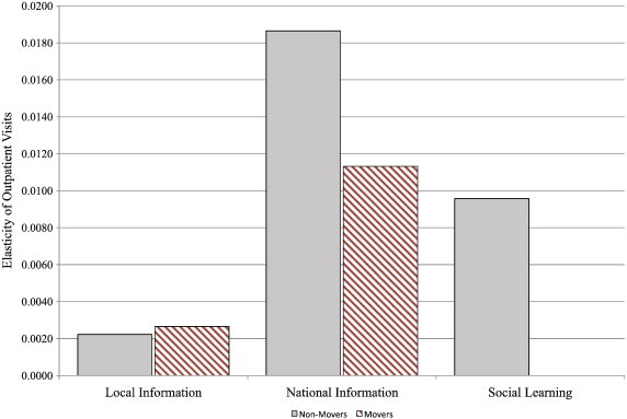
The prevalence response elasticity by information source.
The specifications in Table 4 evaluate the robustness of the peer effect result. We replace the SARS incidence variables with comprehensive time fixed effects. Although the table does not report the coefficients, these regressions also include all levels and pairwise interactions of , as well as the one-year lag of individual visits.19 Column 1 shows the baseline estimate, which is slightly larger than the estimates in Table 3. Columns 2 and 3 incorporate peer group × SARS and peer group × time fixed effects respectively. These more restrictive specifications only increase the magnitude of the peer effect estimate. Column 3 is identified exclusively through the difference between the responses of movers and non-movers within a common peer group. For these results to be spurious, non-movers must experience differentially strong unobservable shocks during SARS.
Table 4.
Robustness under alternative specifications.
| Dependent variable: |
Individual visits |
|||||||
|---|---|---|---|---|---|---|---|---|
| Specification: | Baseline |
2 Visits to join |
Alt. overlap |
Facility groups |
Township groups |
County groups |
||
| (1) | (2) | (3) | (4) | (5) | (6) | (7) | (8) | |
| Change in peer visits × N × SARS | 0.085⁎⁎⁎ | 0.112⁎⁎⁎ | 0.185⁎⁎⁎ | 0.063⁎⁎⁎ | 0.099⁎⁎⁎ | 0.072⁎⁎⁎ | 0.068⁎⁎⁎ | 0.047⁎⁎⁎ |
| (0.012) | (0.015) | (0.052) | (0.007) | (0.025) | (0.010) | (0.007) | (0.004) | |
| Fixed effects: | ||||||||
| Doc. × facility × N, year × period | Yes | – | – | Yes | Yes | Yes | Yes | Yes |
| Doc. × facility × SARS, year × period | – | Yes | – | – | – | – | – | – |
| Doc. × facility × year × period | – | – | Yes | – | – | – | – | – |
| Observations | 79.7 mil | 79.7 mil | 79.7 mil | 47.7 mil | 79.7 mil | 79.7 mil | 79.7 mil | 79.7 mil |
| R2 | 0.103 | 0.111 | 0.323 | 0.076 | 0.105 | 0.102 | 0.103 | 0.102 |
Note: Standard errors appear in parentheses. Standard errors are clustered by the patient's modal township. The dependent variable is measured at time t and all regressors are measures from time t to t − 2. Regressions include all pairwise interactions between SARS, N, and the change in peer visits, as well as individual visits from period t − 26.
p < 0.01.
Columns 4–8 of Table 4 show that the peer effect estimate is robust under several alternative formulations. In Column 4, people must visit a doctor × facility twice during 2001–2003, rather than once, in order to belong to a peer group. Column 5 broadens the definition of a mover by defining a move as a transition across townships with overlap below the 10th percentile rather than the 5th percentile. Columns 6–8 define peer groups by facility, township, or county. Defining peer groups by physician × facility leads to the largest peer effect estimate. The estimate declines if we broaden peer groups further.
In the preceding estimates, a mover is defined as someone with tenure in the community of 1 or 2 years in 2003. We test the sensitivity our results to this definition by varying the tenure cutoff between movers and non-movers. Fig. 9 plots the coefficient on from these regressions, and shows that the peer effect estimate declines smoothly as the definition of a mover is relaxed.
Fig. 9.

The social learning estimate with alternative mover definitions.
Table 5 investigates the timing of the SARS response by category of diagnosis. Instead of treating Quarters 2–4 as a common SARS period, these regressions interact with quarter-of-2003 dummies. Column 1 shows that across all diagnoses, the peer effect is greatest in Quarter 2, followed by Quarter 4. While Quarter 2 coincides with the peak of the epidemic, the result for Quarter 4 is initially surprising because visits fully resumed by the end of Quarter 3. Distinguishing among diagnoses helps to explain this finding. In Columns 2–5, the peer effect estimate is particularly strong for respiratory infections but is much smaller for critical or chronic illnesses. As Fig. 5 highlights, the SARS response for respiratory visits lasted through the end of Quarter 4.
Table 5.
Social learning by diagnosis and quarter of 2003.
| Dependent variable: |
Individual visits |
||||
|---|---|---|---|---|---|
| Type of visit: | All |
Respiratory |
Critical |
Chronic |
Other |
| (1) | (2) | (3) | (4) | (5) | |
| N × change in peer visits: | |||||
| × 2003 Quarter 1 | 0.050⁎⁎⁎ | 0.034⁎⁎⁎ | 0.0031 | − 0.0011 | 0.015 |
| (0.017) | (0.011) | (0.0036) | (0.0023) | (0.0100) | |
| × 2003 Quarter 2 | 0.13⁎⁎⁎ | 0.059⁎⁎⁎ | 0.013⁎⁎ | 0.0035 | 0.061⁎⁎⁎ |
| (0.018) | (0.012) | (0.0057) | (0.0036) | (0.011) | |
| × 2003 Quarter 3 | 0.069⁎⁎⁎ | − 0.0012 | 0.019⁎⁎⁎ | 0.0037 | 0.050⁎⁎⁎ |
| (0.019) | (0.010) | (0.0060) | (0.0033) | (0.013) | |
| × 2003 Quarter 4 | 0.092⁎⁎⁎ | 0.058⁎⁎⁎ | 0.0060 | − 0.00050 | 0.032⁎⁎ |
| (0.023) | (0.014) | (0.0051) | (0.0036) | (0.013) | |
| Observations | 79,663,296 | 79,663,296 | 79,663,296 | 79,663,296 | 79,663,296 |
| R2 | 0.102 | 0.088 | 0.097 | 0.187 | 0.087 |
Note: Standard errors appear in parentheses and are clustered by the patient's modal township. All regressions include peer group fixed effects and year period fixed effects. The dependent variable is measured at time t and all regressors are calculated for time t to t − 2. Critical visits include visits related to pregnancy, abortion, injury, appendicitis, stroke, heart attack, and internal bleeding. Chronic visits include visits related to dialysis, chemotherapy, diabetes, and liver or kidney failure.
p < 0.05.
p < 0.01.
4.2. An alternative identification strategy
This section corroborates our results under an alternative identification strategy. As we explain in Section 2.2, an alternative identifying assumption is that common unobservables do not confound the effect of . We regress vijkt on and separately (as well as v ijkt − 26) according to Eq. (3). The sign of the peer effect estimate is reversed in these regressions because enters negatively. These regressions control for peer group and time fixed effects but cannot utilize peer group × time fixed effects because they exploit inter-group variation.20
| (5) |
Regressions based on this approach appear in Table 6 . Columns 1–4 include SARS incidence, while Columns 5 and 6 include comprehensive time fixed effects. Columns 1, 3, and 5, which most closely conform to Eq. (3), yield peer effect estimates that closely resemble the estimates in Table 3, Table 4.21 In Columns 2, 4, and 6, we control separately for the average current visits of mover and non-mover peers. We also interact these variables with Ni in order to allow for a differential effect for non-movers of among non-mover peers. These regressions show directly that peer effect estimates are insensitive to shocks specific to non-movers, supporting the identifying assumption of our previous approach.22
Table 6.
Regressions that utilize the level of visits as a control.
| Dependent variable: |
Individual visits |
|||||
|---|---|---|---|---|---|---|
| SARS case definition: | Reported |
Probable |
N/A |
|||
| (1) | (2) | (3) | (4) | (5) | (6) | |
| Local SARS incidence | − 0.11⁎⁎⁎ | − 0.085⁎⁎ | − 0.238⁎⁎⁎ | − 0.201⁎⁎⁎ | ||
| (0.023) | (0.037) | (0.040) | (0.073) | |||
| National SARS incidence | − 1.41⁎⁎⁎ | − 2.01⁎⁎⁎ | − 5.13⁎⁎⁎ | − 7.33⁎⁎⁎ | ||
| (0.17) | (0.16) | (0.65) | (0.64) | |||
| Lagged visits of all peers × SARS | − 0.096⁎⁎⁎ | − 0.083⁎⁎⁎ | − 0.097⁎⁎⁎ | − 0.085⁎⁎⁎ | − 0.098⁎⁎⁎ | − 0.083⁎⁎⁎ |
| (0.010) | (0.013) | (0.010) | (0.013) | (0.010) | (0.013) | |
| Current visits of all peers × SARS | 0.053⁎⁎⁎ | 0.054⁎⁎⁎ | 0.052⁎⁎⁎ | |||
| (0.0094) | (0.0094) | (0.010) | ||||
| Current visits of non-mover peers × SARS | ||||||
| – | 0.081⁎⁎⁎ | 0.079⁎⁎⁎ | 0.045⁎⁎⁎ | |||
| (0.014) | (0.014) | (0.012) | ||||
| × N | − 0.057⁎⁎⁎ | − 0.053⁎⁎⁎ | − 0.022⁎ | |||
| (0.013) | (0.013) | (0.012) | ||||
| Current visits of mover peers × SARS | ||||||
| – | 0.0061 | 0.0057 | − 0.0007 | |||
| (0.0065) | (0.0065) | (0.0064) | ||||
| × N | − 0.023⁎⁎ | − 0.023⁎⁎ | − 0.017⁎ | |||
| (0.0093) | (0.0093) | (0.0093) | ||||
| Observations | 79.7 mil | 76.2 mil | 79.7 mil | 76.2 mil | 79.7 mil | 76.2 mil |
| R2 | 0.10 | 0.18 | 0.10 | 0.18 | 0.10 | 0.18 |
Note: Standard errors appear in parentheses and are clustered by the patient's modal township. All regressions include peer group fixed effects. Columns 1–4 include year and period fixed effects. Columns 5 and 6 include year × period fixed effects. The dependent variable is measured at time t and all regressors are calculated for time t to t − 2.
p < 0.10.
p < 0.05.
p < 0.01.
4.3. Chinese New Year
A falsification test based on Chinese New Year further validates the social learning result. During Chinese New Year, both patients and physicians travel to reunite with family, causing a 20–30% decline in health care utilization that is unrelated to social interactions. Chinese New Year represents a combination of supply and demand shocks, both of which threaten the identification of the estimates above. Some offices close and others remain open during Chinese New Year, potentially generating a correlation between Δv ijkt and . If unobservable shocks spuriously drive our findings, then an interaction with Chinese New Year may generate the same pattern. In this section we replace Dt with an indicator for Chinese New Year (Ct) in our main specifications. We avoid any confounding effect of SARS in these regressions by excluding the SARS period. Alternatively, we include interactions with both Dt and Ct in the same regression, which allows us to test whether the “peer effects” estimates for SARS and Chinese New Year are statistically different.
Chinese New Year results based on both identification strategies appear in Table 7 . Column 1 replicates our main specification (Column 1 of Table 4) but replaces SARS with Chinese New Year, while Column 2 includes both SARS and Chinese New Year interactions. The Chinese New Year estimate is negatively rather than positively signed, in contrast to the SARS estimate, which suggests that it does not capture a similar response. An F-test clearly rejects the hypothesis that the Chinese New Year and SARS estimates are the same. Columns 3 and 4 show similar regressions under the identification strategy that controls for current peer visits. Again the Chinese New Year effect is small (7% of the SARS effect) and statistically insignificant. These results indirectly support our methodology by failing to find a spurious peer effect during Chinese New Year.
Table 7.
A falsification test using Chinese New Year.
| Dependent variable |
Individual visits |
|||
|---|---|---|---|---|
| Identification strategy | DD |
Control for peer visits |
||
| (1) | (2) | (3) | (4) | |
| Change in peer visits × N × CNY | − 0.019 | − 0.028⁎⁎ | ||
| (0.015) | (0.014) | |||
| Change in peer visits × N × SARS | 0.10⁎⁎⁎ | |||
| (0.012) | ||||
| Lagged visits of all peers × CNY | − 0.0090 | − 0.0068 | ||
| (0.010) | (0.0098) | |||
| Lagged visits of all peers × SARS | − 0.099⁎⁎⁎ | |||
| (0.010) | ||||
| Equality of CNY and SARS estimates (p-value) | – | < 0.001 | – | < 0.001 |
| Observations | 59.2 mil | 79.7 mil | 59.2 mil | 79.7 mil |
| R2 | 0.105 | 0.103 | 0.105 | 0.103 |
Note: Standard errors appear in parentheses and are clustered by the patient's modal township. All regressions include physician × facility and year × period fixed effects. The specifications in Columns 1 and 2 are consistent with Column 1 of Table 4. Columns 3 and 4 are consistent with Column 5 of Table 6. * p < 0.10.
p < 0.05.
p < 0.01.
5. Dynamic simulation
In this section, we simulate the dynamic response of visits to the SARS epidemic. The response to SARS may have a dynamic component because individuals update their beliefs about SARS risk using information from previous periods, including information from peers. To simulate the dynamic response, we first estimate a regression that allows us to predict visits in the current period based on information from the prior period. Then we simulate the behavior of a hypothetical population in each period and update peer behavior by aggregating individual responses before simulating the next period.
The simulation follows a thought experiment in which we sequentially remove social interactions and peer group shocks from the aggregate response to SARS, ultimately leaving only the response to public information. This exercise allows us to distinguish the relative influence of public information and peer effects. To simulate the path of visits without a given source of information, we zero out the appropriate regression coefficient(s) when predicting individual visits.
5.1. Simulation methodology
In this exercise, we focus on simulating the behavior of non-movers, who we posit experience greater peer effects than movers. Therefore, we simulate peer effects by adding the regression coefficient that captures peer effects among non-movers to regression coefficients that capture the influence of other sources of information on these residents.
The simulation includes four counterfactuals, which we summarize in Table 8 .23 The regression model for all counterfactuals is a variant of Eq. (2) estimated on a combined sample of movers and non-movers.24
| (6) |
Table 8.
Description of simulation counterfactuals.
| Counterfactual | Description | Simulation model |
|---|---|---|
| 1 | Public information + peer group shocks + social learning | |
| 2 | Public information + peer group shocks | |
| 3 | Public information | |
| 4 | No information |
Note: uijkt is an independent draw from a distribution, where is the variance of the residual from the regression model in Counterfactual 1. is the prediction of visits.
We simulate the visits of non-movers by iteratively generating predictions using coefficient estimates that capture the response of non-movers to national SARS prevalence, peer group shocks plus coefficients on the regressors and , which capture peer effects among non-movers.
In the first counterfactual, non-movers respond to public SARS information, peer group shocks, and social interactions. The second counterfactual preserves the response to public information and peer group shocks but shuts down peer effects. We accomplish this by simulating non-mover behavior using the coefficients from the first counterfactual but setting the coefficient on to zero. This approach measures peer effects in a conservative way because it counts the effect of as a peer group shock, even though this coefficient may partially reflect peer effects outside of the SARS period. For the third counterfactual, in which people only respond to public information, the simulation also zeroes out the coefficients on and all associated interactions. National SARS incidence is the only remaining variable that contains information about the epidemic. In the fourth counterfactual, the simulation excludes the response to national SARS incidence by also setting the coefficient on s t n to zero. This scenario provides a benchmark for comparison to the other counterfactuals.
5.2. Simulation results
Fig. 10, Fig. 11 show the paths of aggregate visits and respiratory visits under the counterfactuals described above. The simulation isolates respiratory visits because Fig. 5 and Table 5 indicate that respiratory visits contribute substantially to the overall decline in visits. In each figure, we calculate the ratio of aggregate visits by period under Counterfactuals 1–3 to aggregate visits under Counterfactual 4. The solid black line presents average visits by non-movers per period from our first counterfactual in which non-movers experience peer effects. The dashed line shows the result for the second counterfactual, which excludes the response to peer effects. The difference between this line and the solid line represents the contribution of peer effects to the overall response. Finally the dotted line shows the response under the third counterfactual, which only includes the response to public information. The difference between the dotted line and the dashed line represents the response to unobservable peer group shocks.
Fig. 10.

The simulated path of aggregate visits under alternate scenarios.
Fig. 11.

Simulated path of respiratory visits under alternate scenarios.
Our simulation of visits for all diagnoses suggests that SARS incidence (public information) was the sole driver of the initial, sharp decline in visits. Peer group shocks and peer effects prolonged the decline beyond the peak in SARS incidence. By Period 13 (just after visits reach their nadir), unobservable shocks and peer effects account for nearly half of the continued suppression in visits.25 By the end of the epidemic in Period 16, visits remained almost 20% below normal and peer effects account for roughly one-third of all visit suppression.26 We find qualitatively similar results for respiratory visits in Fig. 11.
6. Discussion
Our goal in this paper is to understand how social interactions may have contributed to the sharp and sustained decline in visits during the SARS epidemic. Although several factors may have contributed to this response, we find that social interactions played a significant role. Others have documented how objectively small risks can trigger disproportionately large responses (Abadie and Gardeazabal, 2003, Blunk et al., 2006, Kraipornsak, 2010). Becker and Rubinstein (2011) suggest that people overreact to unfamiliar risks. In our setting, overreaction does not explain the sharp increase in the coefficient of variation in Fig. 7, while social interactions can explain this pattern. Without a theory of differential overreaction by non-movers, overreaction also fails to explain the differential correlation between the behavior of non-movers and their peers. In our analysis, both public signals and time fixed effects may embody overreaction to SARS. The simulation, which shows similar responses to public information and social interactions, suggests that peer effects contribute in an important way to the response to SARS in Taiwan.
In principle, several forms of social interaction may contribute to the peer effect we observe. We label these mechanisms social learning, imitation, contagion, and congestion. As we discuss in Section 2, social learning is a very plausible cause of a heightened peer effect for non-movers during SARS. In a novel epidemic, people face considerable uncertainty about the risk and severity of the disease, as well as the effectiveness of possible prevention measures. Public signals such as incidence reports only provide a noisy signal of an idiosyncratic risk exposure. People with social connections may demand additional information from peers under these conditions.
Peer imitation may also contribute to the peer effect during SARS. Imitation lacks a consensus definition (Apesteguia et al., 2007), however imitation is distinct from learning because learning involves the transmission of information among peers. A complementarity between individual and peer consumption (either through utility or the budget constraint) may lead to imitation. Complementary utility may lead people to watch the same television shows or wear the same clothing brands as their peers. Complementarity in terms of the budget sets may cause peers to share transportation to common activities. A medical visit is distinct from entertainment or clothing because health is idiosyncratic, and so a peer's health care utilization does not strongly influence someone's utility of a medical visit. Imitation due to cost sharing (e.g. carpooling to medical facilities) could contribute to the peer effect, however this effect would need to become stronger during SARS to contribute to identification, which we do not suspect. Finally, peers could have coordinated with each other in terms of the extent of social distancing. While we cannot rule out this hypothesis, it would be odd to coordinate in this dimension without also communicating SARS risk perceptions.
Contagion of either SARS or other diseases could also contribute to a peer effect. By interacting socially, peers may transmit communicable diseases to one another, causing a positive correlation in their medical visits. SARS prevalence is too low for SARS contagion to have a noticeable effect on our estimates. SARS incidence peaked nationally in Period 10 of 2003, in which there were 270 probable cases. During this period, there were 928,700 outpatient visits, which was 230,300 fewer than Period 10 of 2002, so that SARS diagnoses comprise 0.029% of visits during this period. The maximum of SARS incidence occurs during Period 9 of 2003 in the Jhongjheng District of Taipei City, in which there were 96 probable cases (0.00006 SARS cases per capita), so that SARS diagnoses comprise 0.57% of visits in Jhongjheng during this period. SARS contagion contributes positively to health care utilization during this period, which works against the aggregate decline in visits that we observe. Our estimates are robust if we limit the sample to the 68% of township × period observations with zero SARS incidence.
Non-SARS contagion may also induce a correlation between the medical visits of peers. However this mechanism can only explain a peer effect for visits due to communicable diseases. Table 5 distinguishes between respiratory, chronic, critical and “other” visits. Critical visits include diagnoses of pregnancy, abortion, injury, appendicitis, stroke, heart attack, and internal bleeding, all of which are non-communicable. Chronic visits relate to dialysis, chemotherapy, diabetes or liver failure. “Other” visits include diagnoses that are neither respiratory, chronic, nor critical. This category is also predominately non-communicable. Contagion cannot explain the significant social interactions for critical and other visits in Columns 3 and 5 of Table 5.
Finally, congestion at medical facilities may manifest as a social interaction because patients may crowd each other out at medical facilities. This mechanism bears particular mention because we define peer groups by physician × facility. However congestion creates a negative correlation between the medical visits of peers, which works against the positive peer effect that we observe. Congestion provides another reason (along with our assumption that movers do not interact socially) why we may underestimate social learning.
Although we have assumed that people curtailed medical visits to avoid catching SARS, they may have also had other motivations. Roughly 131,000 people were quarantined during the epidemic (Hsieh et al., 2004), and people with flu symptoms may have feared being quarantined if they visited a doctor's office. Our comparison of movers and non-movers can distinguish between SARS avoidance and quarantine avoidance. A doctor's decision to quarantine, like the decision to close an office, is invariant to the patient's status as a mover.
7. Conclusion
This paper analyzes the behavioral response to the SARS crisis. Our analysis broadens the existing approach to measuring the response to risk by comparing the response to public and private risk signals. Estimates indicate that the response to information from peers and the response to public information have similar elasticities. The social learning mechanism may partially explain why people react more strongly to risks that are novel rather than mundane. Our dynamic simulation indicates that social interactions magnified the behavioral response to SARS risk.
Crises like the SARS epidemic occur with regularity. Past examples include the 9/11 terrorist attacks, the outbreaks of H1N1 and H5N1 flu, and oil spill in the Gulf of Mexico. In 2011, the earthquake and tsunami in Japan forced many residents to assess the risk of radiation exposure. Despite reassuring test results, consumption of Japanese seafood fell dramatically because people worried about radiation (Fukue, 2011, Kelland, 2011). The outbreak of a novel strain of E. coli in Europe in June caused an international scare over Spanish produce before officials traced the outbreak to Germany (Patterson, 2011).
The way people learn from their peers may strongly influence the duration and severity of an emergency. Social learning can cause the perception of risk to deviate from reality in either a positive or negative direction, leading to either an insufficient or excessive private response. By skewing individual risk perceptions, social learning may also influence the demand for public policies related to risk, such as counter-terrorism or nuclear energy initiatives. As a result, authorities may wish to control the extent of social learning about risk. Further research should examine how education campaigns or more precise public signals affect the reliance on information from peers.
Footnotes
We received helpful feedback from Tim Conley, Steven Durlauf, Enrico Moretti, Kaivan Munshi, Kenneth Wolpin, and seminar participants at the University of Chicago, Georgia Tech, Notre Dame, the University of North Carolina, and the University of Pennsylvania. Thanks to Hugh Montag for research assistance. Anup Malani acknowledges financial support from the Samuel J. Kersten Faculty Fund. This study is based in part on data from the National Health Insurance Research Database provided by the Bureau of National Health Insurance, Department of Health and managed by National Health Research Institutes. The interpretation and conclusions contained herein do not represent those of the Bureau of National Health Insurance, Department of Health or National Health Research Institutes.
Visits due to SARS make up 0.029% of national outpatient visits during Period 10 of 2003, in which SARS incidence peaked. We discuss this mechanism further in Section 6.
An examination of mortality data shows that the epidemic coincides with a spike of 520 additional non-SARS deaths, which is over six times the number of deaths from SARS itself. The steep drop in health care utilization during SARS is the most likely reason for this pattern. Widespread avoidance of health care facilities likely reduced SARS transmission and made the outbreak easier to control (Chen, 2003, Lin, 2003).
This assumption also requires type-specific time fixed effects. With this modification, the first term of ξijt is the difference between sijtp,md and . Regression estimates that include type-specific time fixed effects (available from the authors) are equivalent to the estimates in Section 4. The insensitivity of our estimates to type-specific time fixed effects suggests the first element of ξ is not a serious confound.
The mortality risk calculation assumes conservatively that all SARS deaths arise because of outpatient visits. Consistent with the extreme response, Liu et al. (2005) find that the VSL associated with avoiding SARS risk is several times greater than conventional VSL measurements from Taiwan.
Critical visits include visits related to pregnancy, abortion, injury, appendicitis, stroke, heart attack, and internal bleeding. Chronic visits include visits related to dialysis, chemotherapy, diabetes, and liver or kidney failure.
Patients with mild respiratory illnesses may have also feared that doctors would place them in quarantine (Hsieh et al., 2005). As a respiratory condition, SARS could also have increased respiratory visits among people concerned about possible exposure.
Confirmatory diagnostic tests for SARS did not become available until midway through the epidemic. Even once these tests arrived, authorities did not provide immediate confirmation of SARS infection. Therefore, people did not generally have information about confirmed SARS incidence.
Published evidence of this phenomenon from countries other than the US is extremely limited. Anecdotally, referrals are especially important in Taiwan because there are few institutional restrictions (such as HMO networks) on the choice of physician.
If group membership requires two rather than one visit, then 85% of the population belongs to at least one group and the median number of groups per person is 4. Quartiles of the group size distribution occur at 6, 29, and 115 people.
The identification strategy exploits heterogenous exposure to social interactions among subsets of the peer group. Cohen-Cole (2006) and Blume et al. (2011, Theorem 2) derive the conditions under which this approach is valid. Despite the superficial similarity, this strategy is distinct from Gaviria and Raphael (2001), who test the endogeneity of school choice by comparing movers and non-movers.
This dichotomy between movers and non-movers does not conflict with Munshi's (2003) finding that international migrants with larger destination networks have better outcomes. Munshi compares migrants from different origin communities within the same city, and does not claim that migrants have larger networks than longtime destination residents.
As a baseline, townships have low overlap if they fall below the fifth percentile of the overlap distribution, so that less than 0.17% of patients visit doctors in both townships. As we show below, results are robust to using the tenth percentile of overlap (0.92%) as an alternative cutoff.
We compute p-values by regressing each variable on a non-mover dummy during the non-SARS period and apply the same probability weights that we use in our regressions below. Income data based on BNHI estimates of earnings by occupation category are available for 62% of the sample.
Because visits are bounded by zero, the decline in visits mechanically reduces the standard deviation. The coefficient of variation partially corrects for this issue.
We control for vijkt − 26 rather than use ∆vijkt as the dependent variable in order to avoid endogeneity due to serial correlation in individual risk perceptions. If perceptions are serially correlated, then lags of vijkt belong as controls in the specification. However, these lags are functionally dependent upon vijkt − 26. Moving vijkt − 26 to the right hand side is the most direct solution to this problem.
The use of a peer group fixed effect leads to bias in the coefficient on the lagged dependent variable. However, Hsiao (2003, p. 72) notes that the bias vanishes as T → ∞. With 78 time periods, this setting features an unusually long panel. Moreover, bias in β4 is unlikely to contaminate the other coefficients: the pairwise correlations of vijkt − 26 with sl, sn, and are 0.002, 0.007, and − 0.021 respectively.
An estimate that incorporates non-mover × time fixed effects (available from the authors) is comparable to these estimates. This finding provides a basis for the second identifying assumption on page 9.
To observe movers' visits to their 2003 peer groups (a necessary aspect of the non-mover difference-in-difference), we must construct peer groups and measure behavior with the same raw data from 2001 to 2003. In regressions that control for , we can construct peer groups based on utilization prior to 2001. Defining peer groups based on 1999–2000 utilization yields similar results.
One mechanism that may induce a negative correlation between vijkt and is regression toward the mean. Stochastic shocks may elevate visits in period t − 26 and suppress visits in period t. By conditioning on vijt − 26, our regressions control for the individual effect of stochastic shocks in period t − 26. Because of the interaction with Dt, these shocks would need to become stronger during SARS to cause a spurious correlation.
The distribution of peer visits is approximately binomial because 99.6% of people visit no more than once per period; therefore is nearly a sufficient statistic for the distribution of visits by peers. Conditioning on can control for aspects of the visit distribution that the mean does not capture. Estimates that included squared peer visits are very similar to the estimates in Table 6.
This exercise is based on the following algorithm. First, we create a simulation data set with 1000 hypothetical doctor's offices, each populated with 61 patients, the median size of peer groups in the regression sample. The simulation data set spans the period from 2002 to 2003. For each person, the number of visits during period t in 2002 equals the mean of this variable for movers in the regression sample. Beginning with the first period in 2003, we construct vijkt using and vijkt − 26 based on lagged data according to the requirements of each counterfactual.
Simulation regressions deviate from our earlier regressions in two important ways. We construct the regressors as sums over periods t − 2 and t − 1, rather than t − 2 to t, to avoid the need to determine vijkt and jointly. Our regression eliminates the need to assign simulated people to actual townships by omitting local SARS incidence, for which the effect is small.
Visits in our simulation closely track the actual decline in visits by movers, for whom all visits fell by around 25% and respiratory visits fell by around 60%.
This result differs slightly from the finding in Table 5 that peer effects had the largest impact in Quarters 2 and 4. This difference most likely arises because the simulation uses a single dummy for the SARS period (Quarters 2–4), while regressions in the table use separate dummies for each quarter.
People may sample peers' beliefs by communicating directly or by observing behaviors like the change in health care utilization, which indicate beliefs. Ellison and Fudenberg (1995) and Offerman and Schotter (2009) develop models of social learning from peer behavior.
Suppose the separate influence of an individual's private and prior information is ϕprivsijtpriv + ϕpriorsij(t − 1), where sijtpriv is private information, sij(t − 1) is prior information and the ϕ's are their respective weights. In Eq. (7), we define sijtp = sijtpriv + (ϕprior/ϕpriv)sij(t − 1) and ϕ2 = ϕpriv.
A large Nj assumption is reasonable because the median peer group size is 55 in our data. Limiting the sample to only large networks, for which this assumption is most valid, does not affect our results.
Therefore, if the two types place the same weight on peers' information, then they place the same weight on private information, i.e., ϕ2nm = ϕ2m ⇔ ϕ3nm = ϕ3m. If movers place less weight on peers' private information, they shift only a portion of that weight to private information, i.e., 0 ≤ ϕ2m − ϕ2nm ≤ − (ϕ3m − ϕ3nm).
The second assumption implies that the full derivative of ϕ3 / (ϕ2 + ϕ3) is positive, even accounting for shift in weight from peers' information to and own private information and lagged peers' beliefs.
Without loss of generality, we ignore the dynamic effects of current health decisions. Our approach can incorporate these effects by reinterpreting the contemporaneous utility function as a value function that embeds future optimizing behavior.
Appendix A. A model of learning about SARS risk
In this appendix, we provide more formal motivation for our empirical approach with a theoretical framework that relates learning and health care utilization. The model highlights the threats to identification and provides an interpretation of the regression coefficients. We first present a simple model of individual belief formation about SARS risk from different information sources that may be empirically observable or unobservable. We then incorporate the decision to seek health care and illustrate the conditions under which a person's observable change in medical visits over time proxies for his perception of SARS risk.
A.1. Learning about SARS risk
People are indexed by i and belong to peer groups that are indexed by j and have size Nj. Each person decides whether to visit the doctor during period t. By visiting, the patient faces perceived risk s ijt ∈ [0, 1] of contracting SARS and dying.
People learn about sijt by observing realizations of this parameter from three data sources. First, the government draws a sample from the distribution of SARS risk. Specifically, it tracks new SARS cases and reports the mean SARS incidence, s jt c ∈ [0, 1], which is a common public signal of SARS risk. Second, people obtain a private estimate of SARS risk. This estimate reflects personal risk factors, such as the frequency of contact with others and use of a mask outdoors. The individual's private signal may be correlated with the common signal or his prior. Third, people sample their peers' estimates of SARS risk, {s ¬ ijt}, where ¬ i indicates individuals other than i.27
Using these information sources, individuals update their prior beliefs using Bayes' theorem. People assume that SARS is distributed binomially in the population. This implies that the posterior probability of an individual catching SARS is a linear weighted average of the means from different data sources (Jewell, 1974) and their priors. For tractability, we make two assumptions about these weights. First, each person places identical weight on the private information of different peers. Second, all individuals place the same weight on each information source. In addition, we define the composite influence of an individual's prior information and his priors as s ijt p.28 This definition does not compromise generality because we proceed under the conservative assumption that s ijt p is not observed. Given these assumptions and our definition, we can represent each agent's learning process with the following linear function.
| (7) |
where is the average beliefs of peers and Ij is the set of individuals in peer group j. The weights, ϕ, are increasing in the reliability and precision of the signal. Our empirical objective is to test whether individual posterior beliefs on SARS risk give positive weight to the common signal (ϕ 1 > 0) or peers' beliefs (ϕ 3 > 0).
Our primary empirical challenges are that the beliefs of peers depend on the beliefs of an individual (the reflection problem), generating endogeneity bias, and that the private signals of person i, and thus the composite input s ijt p, is unobservable. The first issue, the learning feedback between the individual and the group, only threatens identification if groups are small. In small groups, an individual's risk perception can have a meaningful impact on the average group risk perception. This impact vanishes, however, as group size increases: . In our data, the median peer group size is 55. Therefore, it is reasonable to assume that Nj is large.29 Under this assumption, the individual perception becomes:
| (8) |
The equation above still cannot be estimated because we do not observe person i's independent private information. Dropping s ijt p, we could estimate a hypothetical regression of the individual's risk perception on the common signal and group risk perceptions.
| (9) |
where ζ ijt = ϕ 3 s ijt p. Because person i's private signal and prior beliefs appear in Eq. (8) but are omitted variables in Eq. (9), the coefficients reflect omitted variable bias.
| (10) |
| (11) |
In these expressions, (γ 1, γ 3) are coefficients from hypothetical regressions of the omitted variable s ijt p on the regressors in Eq. (9): .
Our empirical approach addresses this omitted variable bias through a difference-in-difference comparison of long time residents (non-movers) and recent arrivals (movers) within a peer group. Movers, who have fewer social connections, place weakly less weight on data from peers than non-movers: ϕ 3 m ≤ ϕ 3 nm. The difference-in-difference estimator can detect social learning (ϕ 3 > 0) despite omitted variable bias in Eq. (11) under two assumptions. First, movers and non-movers obtain private signals and peers' information in the same way, so the correlation between different sources of data is identical for movers and non-movers, i.e., γ 3 m = γ 3 nm. Second, movers and non-movers follow the same Bayesian updating process in Eq. (7).30 These assumptions imply that the coefficient on average peer beliefs in Eq. (11) is larger for the non-mover group only if ϕ 3 nm > 0.
The differential response of non-movers is
This is positive only in a subset of cases where ϕ 3 nm > 0: when non-movers place positive weight on peers' information and movers place much less weight on that information. If movers place less weight on peers' information, they must place more weight on own private information, making the second term negative. For the differential response to be positive, the first term must be sufficiently positive, which is possible only if ϕ 3 nm > > ϕ 3 m.31 In other cases where ϕ 3 nm > 0 or when ϕ 3 nm = 0, the differential is easily verified to be negative or zero.
A.2. Using change in visits as a proxy for perceived risk
To estimate regression (Eq. (9)), we must either observe or proxy for individual and group risk perceptions sijt and . Here we motivate the use of the change in medical visits over time as a proxy for perceived risk and explain what a regression employing this proxy reveals about the structural parameters.
When deciding whether to see the doctor, a person compares his level of illness to his perceived cost of a visit. In general, this cost includes the copayment (which is less than US$5 per visit) and the cost of transportation to the medical facility. During SARS, the cost also includes the risk of contracting SARS during the visit. Holding illness and other costs constant, a change in visits indicates a change in the perceived SARS risk.
More formally, people receive utility from health and other consumption, hijt and xijt, respectively. In each period, people experience a health shock, dijt ≥ 0, and must decide whether to seek medical care, vijt ∈ {0, 1}. A visit to the doctor restores the patient to his baseline health, but requires him to pay a copayment ct. During the SARS epidemic, people also face the risk that a visit may cause them to catch SARS and die. After normalizing the utility from death to be zero, the expected utility from visiting and not visiting the doctor are:32
| (12) |
| (13) |
A person seeks care if the value of alleviating his illness exceeds the cost of treatment: EU[v ijt = 1] > EU[v ijt = 0]. Taking logs yields to the following equivalent expression.
In this formulation, the probability of a visit depends upon the person's health status and his perceived SARS risk.
An observer wishing to interpret the change in visits as an indicator of perceived risk must account for secular trends in health. To satisfy this requirement, we assume that the difference in log utility from seeking care rather than not seeking care is a trend-stationary function of the person's age: ln u(h ijt, x ijt − c t) − ln u(h ijt − d ijt, x ijt) = μ ij + ga ijt − e ijt, where aijt is the person's age.33 The error term, eijt, is identically and independently distributed throughout the population, with mean zero, cumulative distribution F(e), and density f(e). Under this formulation, people experience idiosyncratic health shocks with a mean that linearly increases with age. The first expression below shows the probability of a visit under these assumptions. In the second expression, we apply a first-order Taylor-series expansion at a suitable common point, , in the distribution of eijt, and incorporate the approximation that ln(1 − s ijt) ≈ − s ijt for small values of sijt.
| (14) |
| (15) |
The probability of a visit is thus an affine transformation of SARS risk, the idiosyncratic health endowment, and age.
The first difference of this probability is our proxy for an individual's perceived SARS risk. We subtract the number of visits during a comparable pre-SARS period (so s ij(t − k) = 0) from the number of visits in the index period. The change in visits, Δv ijt = v ijt − v ijt − k, nets out the time-constant health endowment and . The coefficient on age becomes a fixed effect because the increase in age is constant for any first difference. Likewise, the change in average peer visits, , proxies for the average risk perception of the peer group.
| (16) |
| (17) |
A person who is familiar with and the effect of age on health, g, can infer sijt and from the change in individual and group visits, respectively.
A.3. Merging the model of learning with the proxy for beliefs
Our empirical strategy uses these proxies to estimate a version of the hypothetical regression in Eq. (9):
| (18) |
By substituting in the expressions for Δv ijt, , sijt and , we find that and have the following structural interpretations.
| (19) |
| (20) |
Although the system (which also includes an expression for ) is not identified, a difference-in-difference estimator that compares movers and non-movers provides a test whether people learn from public information and from peers. A significant value of indicates that people learn from public information, while a significant value of indicates that people learn from their peers. The signs on these coefficients differ because an increase in indicates less risk while an increase in s jt c indicates greater risk.
Eq. (19) also shows that incorrectly estimates the response to public information ϕ 1. In the special case where the common signal is uncorrelated with private information or prior beliefs, however, a complementary regression of the change in individual visits on just the common signal avoids omitted variable bias and identifies ϕ 1.
| (21) |
The coefficient on the common signal has the following structural interpretation:
Using this coefficient estimate rather than leads to a larger estimate of learning from public information. It is also more accurate if the common signal is uncorrelated with private information or prior beliefs. A regression based on Eq. (21) proves useful for the dynamic simulation in Section 5, where it serves as a predictive model that better captures the response to public information.
References
- Abadie Alberto, Gardeazabal Javier. The economic costs of conflict: a case study in the Basque Country. Am. Econ. Rev. 2003;93(1):113–132. (March) [Google Scholar]
- Ahituv Avner, Joseph Hotz V., Philipson Tomas. The responsiveness of the demand for condoms to the local prevalence of HIV. J. Hum. Resour. 1996;31(4):869–897. (September) [Google Scholar]
- Apesteguia Jose, Huck Steffan, Oechssler Jörg. Imitation — theory and experimental evidence. J. Econ. Theory. 2007;136:217–235. [Google Scholar]
- Banerjee Abhijit. A simple model of herd behavior. Q. J. Econ. 1992;107(3):797–817. [Google Scholar]
- Becker Gary, Rubinstein Yona. Centre for Economic Performance (LSE) Discussion Paper. 2011. Fear and the Response to Terrorism: An Economic Analysis. [Google Scholar]
- Bikchandani Sushil, Hirschleifer David, Welch Ivo. A theory of fads, fashion, custom, and cultural change as information cascades. J. Polit. Econ. 1992;100(5):992–1026. (October) [Google Scholar]
- Blalock Garrick, Kadiyali Vrinda, Simon Daniel H. Driving fatalities after 9/11: a hidden cost of terrorism. Appl. Econ. 2009;41:1717–1729. [Google Scholar]
- Blume Lawrence, Brock William, Durlauf Steven, Ioannides Yannis. Identification of Social Interactions. In: Benhabib Jess, Jackson Matthew., editors. vol. 1B. 2011. pp. 853–964. (Handbook of Social Economics). [Google Scholar]
- Blunk Scott, Clark David, McGibany James. Evaluating the long-run impacts of the 9/11 terrorist attacks on US domestic airline travel. Appl. Econ. 2006;38(4):363–370. (March) [Google Scholar]
- Card David, Dobkin Carlos, Maestas Nicole. Does medicare save lives? Q. J. Econ. 2009;124(2):597–636. doi: 10.1162/qjec.2009.124.2.597. (May) [DOI] [PMC free article] [PubMed] [Google Scholar]
- Chen Wu-Tsung. Improve safety through fewer hospital visits. Kaohsiung Med. Univ. Newslett. 2003;23(2) (July) [Google Scholar]
- Cheng Tsung-Mei. Taiwan's new national health insurance program: genesis and experience so far. Health Aff. 2003;22(3):61–76. doi: 10.1377/hlthaff.22.3.61. (May/June) [DOI] [PubMed] [Google Scholar]
- Chou Ji, Kuo Nai-Fong, Peng Su-Ling. Potential impacts of the SARS outbreak on Taiwan's economy. Asian Econ. Pap. 2004;3(1):84–99. (Winter) [Google Scholar]
- Cohen-Cole Ethan. Multiple groups identification in the linear-in-means model. Econ. Lett. 2006;92(2):157–162. (August) [Google Scholar]
- Conley Timothy, Udry Christopher. Learning about a new technology: pineapple in Ghana. Am. Econ. Rev. 2010;100(1):35–69. (March) [Google Scholar]
- Currie Janet, Gruber Jonathan. Health insurance eligibility, utilization of medical care, and child health. Q. J. Econ. 1996;111(2):431–466. (May) [Google Scholar]
- de Paula Aureo, Shapira Gil, Todd Petra. Penn Institute for Economic Research Working Paper 11-033. 2011. How Beliefs about HIV Status Affect Risky Behaviors: Evidence from Malawi. [Google Scholar]
- Delavande Adeline, Kohler Hans-Peter. The impact of HIV testing on subjective expectations and risky behavior in Malawi. Demography. 2012;49(3):1011–1036. doi: 10.1007/s13524-012-0119-7. (August) [DOI] [PMC free article] [PubMed] [Google Scholar]
- Deri Catherine. Social networks and health service utilization. J. Health Econ. 2005;24(6):1076–1107. doi: 10.1016/j.jhealeco.2005.03.008. (November) [DOI] [PubMed] [Google Scholar]
- Ellison Glenn, Fudenberg Drew. Word-of-mouth communication and social learning. Q. J. Econ. 1995;110(1):93–125. (February) [Google Scholar]
- Foster Andrew, Rosenzweig Mark. Learning by doing and learning from others: human capital and technical change in agriculture. J. Polit. Econ. 1995;103(6):1176–1209. [Google Scholar]
- Fukue Natsuko. The Japan Times. 2011. Fisheries Hit By Safety Fears. (April 14) [Google Scholar]
- Gaviria Alejandro, Raphael Steven. School-based peer effects and juvenile behavior. Rev. Econ. Stat. 2001;83(2):257–268. (May) [Google Scholar]
- Gersovitz Mark, Hammer Jeffrey. Infectious diseases, public policy, and the marriage of economics and epidemiology. World Bank Res. Obs. 2003;18(2):129–157. (September) [Google Scholar]
- Glaeser Edward, Sacerdote Bruce, Scheinkman Jose. Crime and social interactions. Q. J. Econ. 1996;111(2):507–548. (May) [Google Scholar]
- Gong Erick. HIV testing and risky sexual behavior. Econ. J. 2014 (forthcoming) [Google Scholar]
- Graham Bryan. Identifying social interactions through conditional variance restrictions. Econometrica. 2008;76(3):643–660. (May) [Google Scholar]
- Hammitt James, Liu Jin-Tan. Effects of disease type and latency on the value of mortality risk. J. Risk Uncertain. 2004;28(1):73–95. [Google Scholar]
- Hoerger T.J., Howard L.Z. Search behavior and choice of physician in the market for prenatal care. Med. Care. 1995;33(4):332–349. doi: 10.1097/00005650-199504000-00002. [DOI] [PubMed] [Google Scholar]
- Hsiao Cheng. Cambridge University Press; 2003. Analysis of Panel Data. [Google Scholar]
- Hsieh Ying-Hen, Chen Cathy W.S., Hsu Sze-Bi. SARS outbreak, Taiwan, 2003. Emerg. Infect. Dis. 2004;10(2):201–206. doi: 10.3201/eid1002.030515. (February) [DOI] [PMC free article] [PubMed] [Google Scholar]
- Hsieh Ying-Hen, King Chwan-Chuan, Chen Cathy W.S., Ho Mei-Shang, Lee Jen-Yu, Liu Feng-Chi, Wu Yi-Chun, Julian Wu Jiunn-Shyan. Quarantine for SARS, Taiwan. Emerg. Infect. Dis. 2005;11(2):278–282. doi: 10.3201/eid1102.040190. (February) [DOI] [PMC free article] [PubMed] [Google Scholar]
- Huang Chao-Hsi. Star News. 2003. Isatidis Radix Sold for 80 Times its Original Price. Gold Thread, Fang Feng, and Jinyinhua Hard to Purchase. (May 5) [Google Scholar]
- Jackson Matthew. Networks and economic behavior. Annu. Rev. Econ. 2009;1 [Google Scholar]
- Jewell William. Credible means are exact Bayesian for exponential families. Astin Bull. 1974;8:77–90. [Google Scholar]
- Kelland Kate. Reuters News. 2011. Japan Radiation Fears Mask Worse Threats to Health. (March 16) [Google Scholar]
- Ko Chih-Hung, Yen Cheng-Fang, Yen Ju.-Y.u., Yang Ming-Jen. Psychosocial impact among the public of the severe acute respiratory syndrome epidemic in Taiwan. Psychiatry Clin. Neurosci. 2006;60:397–403. doi: 10.1111/j.1440-1819.2006.01522.x. [DOI] [PubMed] [Google Scholar]
- Kraipornsak Paitoon. The outbreak of avian influenza and chicken consumption in Thailand. Res. Bus. Econ. J. 2010;2:1–18. [Google Scholar]
- Lakdawalla Darius, Sood Neeraj, Goldman Dana. HIV breakthroughs and risky sexual behavior. Q. J. Econ. 2006;121(3):783–821. (August) [Google Scholar]
- Lin Ya-Li. Liberty Times. 2003. Facing the Urgent Threat of SARS, Eight Cities and Counties Regulate Inpatient Visits. (May 22) [Google Scholar]
- Liu Jin-Tan, Hammitt James, Wang Jung-Der, Tsou Meng-Wen. Valuation of the risk of SARS in Taiwan. Health Econ. 2005;14(1):83–91. doi: 10.1002/hec.911. (January) [DOI] [PubMed] [Google Scholar]
- Manski Charles. Identification of endogenous social effects: the reflection problem. Rev. Econ. Stud. 1993;60:531–542. [Google Scholar]
- Manski Charles. Economic analysis of social interactions. J. Econ. Perspect. 2000;14(3):115–136. (Summer) [Google Scholar]
- Moretti Enrico. Social learning and peer effects in consumption: evidence from movie sales. Rev. Econ. Stud. 2011;78(1):356–393. (January) [Google Scholar]
- Munshi Kaivan. Networks in the modern economy: Mexican Migrants in the US labor market. Q. J. Econ. 2003;118(2):549–599. (May) [Google Scholar]
- Munshi Kaivan. Social learning in a heterogeneous population: technology diffusion in the Indian Green Revolution. J. Dev. Econ. 2004;73:185–213. [Google Scholar]
- National Policy Foundation . 2003. The Impact of the SARS Epidemic on the Travel and Transportation Industry. (May) [Google Scholar]
- Offerman Theo, Schotter Andrew. Imitation and luck: an experimental study on social sampling. Games Econ. Behav. 2009;65:461. [Google Scholar]
- Oster Emily, Thornton Rebecca. Menstruation, sanitary products, and school attendance: evidence from a randomized evaluation. Am. Econ. J. Appl. Econ. 2011;3(1):91–100. [Google Scholar]
- Patterson Tony. The Independent (London) 2011. E. coli Panic Grips Germany While Britain Waits Nervously. (June 4) [Google Scholar]
- Philipson Tomas, Posner Richard. A Theoretical and Empirical Investigation of the Effects of Public Health Subsidies for STD Testing. Q. J. Econ. 1995;110(2):445–474. [Google Scholar]
- Siu Alan, Wong Y.C. Richard. Economic impact of SARS: the case of Hong Kong. Asian Econ. Pap. 2004;3(1):62–83. [Google Scholar]
- Thornton Rebecca. The demand for and impact of learning HIV status: evidence from a field experiment. Am. Econ. Rev. 2008;98(5):1829–1863. doi: 10.1257/aer.98.5.1829. [DOI] [PMC free article] [PubMed] [Google Scholar]
- Tu Ha, Lauer Johanna. Center for Studying Health System Change Research Brief; 2008. Word of Mouth and Physician Referrals Still Drive Health Care Provider Choice. (December) [PubMed] [Google Scholar]
- Welch Ivo. Sequential sales, learning, and cascades. J. Financ. 1992;47(2):695–732. (July) [Google Scholar]
- WHO Case definitions for surveillance of Severe Acute Respiratory Syndrome (SARS) 2003. http://www.who.int/csr/sars/casedefinition/en/