

Abstract
In many hospitals, isolation rooms are used to contain patients who are highly infectious, and the spread of air and bacteria within the isolation room is closely relates to room air distribution. This article uses the computational fluid dynamics (CFD) method to investigate the effects of a moving person and the opening and closing of a sliding door on room air distribution, including velocity, pressure and contaminant fields. Dynamic meshes are employed to simulate the movement of the walking person and sliding door. According to numerical results, the impact of those moving objects on room air distribution is addressed in this study.
Keywords: Isolation room, Airflow simulation, Computational fluid dynamics (CFD), Dynamic mesh, Finite-volume method
Nomenclature
- A
area
- C
contaminant concentration
- C0
maximum contaminant concentration at the mouth
- Cd
C/C 0
- Cp
specific heat
- D
mass diffusion coefficient
- Dh
hydraulic diameter
- g
gravity acceleration
- H
specific enthalpy
- h
height of the isolation room
- I
turbulence intensity
- k
turbulence kinetic energy
- ΔP
pressure difference between the isolation room and anteroom
- S
source term
- T
temperature
- Δt
time step
- u
velocity component in the x-direction
- uavg
mean flow velocity
velocity vector
- V
volume
- v
velocity magnitude
- υ
velocity component in the y-direction
- X, Y, Z
Cartesian coordinates
Greek symbols
- Γeff
effective diffusion coefficient
- β
thermal expansion coefficient
- ε
turbulence kinetic energy dissipation rate
- λ
thermal conductivity
- μ
dynamic viscosity
- ρ
density
- φ
dependent variable
Superscripts
- n
current time level
next time level
Subscripts
- ref
reference value
- 0
reference value
1. Introduction
In many hospitals, isolation rooms for diseases, such as tuberculosis (TB) and severe acute respiratory syndrome (SARS), are usually arranged for treating patients who are highly infectious. The quality of the overall hospital environment relies on the air-conditioning design, such as the control of temperature, humidity, pressure, and indoor air quality (IAQ), etc. Special design of air-conditioning and ventilating systems to maintain negative pressure within isolation rooms must be employed to protect health care workers and other patients. The purpose of maintaining negative internal pressure is to restrain the air and bacteria within isolation rooms. Suitable control of internal pressure and airflow direction within isolation rooms can effectively isolate infected patients and inhibit the spread of air and bacteria.
It is known that the design of isolation rooms has a close relationship with indoor air movement, and many studies have been done on indoor air movement. These studies generally focused on analyzing the indoor air distribution, turbulence characteristics, thermal comforts, IAQ, etc. [1], [2]. Two methods, including experimental measurement and computational fluid dynamics (CFD) simulation, were commonly adopted in these studies. Because experimental measurement required a lot of time and expense, CFD simulation became one of the most economic and efficient tools to investigate indoor air movement. In order to make the simulation results reliable and accurate, much effort [3], [4], [5], [6], [7] was put into (i) inspecting the influence of different turbulence models, and various numerical schemes and algorithms on the simulation results; and (ii) the verification of simulation and experimental results. Unfortunately, there is still no unique turbulence model, numerical scheme or numerical algorithm valid for solving all indoor air motions. Hence, choosing a reliable turbulence model, numerical scheme and numerical algorithm can increase the accuracy of simulating indoor air motion.
Poor IAQ often results in “sick-building syndrome” or “sick-house syndrome”, which is detrimental to the health of human beings, and the IAQ problem has become one of the most important research topics in the HVAC industry recently. For instance, Gan [8] employed the CFD method to evaluate the effect of different air supply systems on indoor air distribution, thermal comfort, ventilation effectiveness and IAQ. The numerical results showed that the upward displacement ventilation yielded better IAQ than other systems. Gan and Awbi [9] adopted the concept of age of air to assess the performance of air distribution systems, including IAQ and ventilation efficiency. Chung and Rankin [10] performed both experimental and numerical studies to evaluate the ventilation efficiency in a model room. They focused on the effect of the relative positions between air supply and return as well as location of partitions on the contaminant decay within a model room. Lee and Awbi [11] also performed a similar study using experimental and numerical methods. Within a model room, Hyun and Kleinstreuer [12] used the CFD simulation to examine the influence of airflow from different directions on the spread of carbon dioxide exhaled by a standing human. Bjørn and Neilson [13] investigated the airflow interaction and contaminant transport between two breathing persons, a condition important in isolation rooms.
Related to the investigation of room air distribution affected by human bodies, most previous studies focused on the influence of stationary human bodies, and few studies [14] discussed the influence of moving objects on the indoor air distribution. However, moving objects usually disturb the air distribution and result in the fluctuations of velocity, pressure, temperature, and concentration within the isolation room. The objective of this article is to use the CFD method to investigate the effects of a moving person and the movement of a sliding door on the air distribution, including velocity, pressure and contaminant fields, within the isolation room.
2. Numerical methodology
In this study, the CFD software FLUENT [15] is utilized to simulate room airflow distribution, and the numerical model is based upon the finite-volume method [16]. The governing equations, including continuity, momentum, energy, contaminant, and turbulence equations obey the principle of conservation and can be expressed in the following general form:
| (1) |
where ρ is the density, φ the dependent variable, the velocity vector, the effective diffusion coefficient, and Sφ the source term. The parameters φ, , and Sφ employed in continuity, momentum, energy, contaminant, and turbulence equations are listed in Table 1 .
Table 1.
Terms, coefficients and constants used in Eq. (1)
| Equation | φ | Γφ,eff | Sφ |
|---|---|---|---|
| Continuity | 1 | 0 | 0 |
| Momentum | μeff | ||
| Energy | H | λeff/Cp | 0 |
| Contaminant | C | ρDeff | 0 |
| Turbulence kinetic energy | k | ||
| Turbulence kinetic energy | ε | ||
| Dissipation rate | |||
| H = Cp(T-Tref) | C1=1.44 | ||
| C2=1.92 | |||
| Cμ=0.09 | |||
| σk=1.0 | |||
| σε=1.3 | |||
| Prt=0.85 | |||
| Sct=0.7 | |||
The diffusion–convection term of Eq. (1) is discretized by the QUICK scheme and the implicit method is used to discretize the transient term. After Eq. (1) is discretized, the general discretized equation can be written as
| (2) |
where a p and a nb are discretized coefficients, and b is the discretized source term. In Eq. (2), subscript p represents the grid point under consideration and nb indicates the neighbors of grid point p.
By employing the iterative scheme of a point implicit (Gauss–Seidel) linear equation solver in conjunction with an algebraic multigrid (AMG) method, the pressure, velocity, temperature, contaminant, and turbulence fields can be solved from Eq. (2). During the iterative procedure, the semi-implicit method for pressure-linked equations—consistent (SIMPLEC) algorithm is employed to solve the pressure–velocity coupling equations.
Regarding the boundary conditions, no-slip condition is used at the wall, and the standard wall functions for the turbulence model are adopted to link the solution variables at the near-wall cells and the corresponding quantities near the wall. To resolve reliable turbulence phenomena near the wall, the grid nearest to the wall falls into the logarithmic layer (that is, ). Moreover, the turbulence kinetic energy k and the turbulence kinetic energy dissipation rate ε employed in air supply and air outlet are calculated by the following equations:
| (3) |
| (4) |
| (5) |
where u avg is the mean flow velocity, I the turbulence intensity, D h the hydraulic diameter and .
To simulate room air distribution affected by the moving person and the opening and closing of the sliding door, dynamic meshes are employed in the numerical simulation. Basic conservation equations of dynamic meshes are described as follows: within an arbitrary control volume V, as its boundary moves, the integral form of governing equation is given by
| (6) |
where is the boundary of control volume V and is the grid velocity of the moving mesh. The transient term of Eq. (6) can be discretized by the following formula
| (7) |
where the superscripts n and represent the current and next time level, respectively. The volume of the control volume at level is calculated by
| (8) |
where dV/dt is the volume derivative with respect to time, which needs to obey the grid conservation law. It can be found by
| (9) |
| (10) |
where n f is the number of faces surrounding the control volume, the area vector of the j face, and δVj is the volume swept by the face j over the time step Δt.
3. Results and discussion
Dynamic analysis of room air distribution within the isolation room, including the effects of a moving person and the opening and closing of the sliding door, is performed numerically in this study. The geometry of two simulating cases is displayed in Figs. 1(a) and (b) .
Fig. 1.
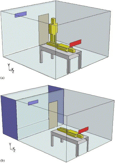
(a) Physical configuration of the model room for the case of a moving person. (b) Geometry of the isolation room and anteroom for the case of the movement of a sliding door.
3.1. Case A: Effect of a moving person
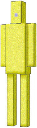
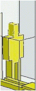
As shown in Fig. 1(a), a model room with the volume of 4×4×2.5 m3 is adopted as the simulated example. The sizes of air supply, air outlet, the moving person, the patient, and the sickbed are listed in Table 2a, Table 2b, Table 2c . The air change rate of the model room is assumed to be twelve. The temperature and turbulence intensity at the air supply are given by 295.15 K and 20%, respectively. The boundary condition of pressure outlet is specified at the air outlet. The pressure outlet represents that the static pressure is given at that boundary and all other flow quantities are extrapolated from the flow in the interior. In order to keep negative internal pressure, static pressure of −8 Pa and turbulence intensity of 10% are given at the pressure outlet. The no-slip condition is applied to all solid surfaces. All boundary walls of the model room are assumed to be adiabatic. Although thermal boundary layer exists on the surface of the moving person, the heat dissipation is not much in a short period of time. Therefore, the moving person is assumed to be adiabatic. The only heat source is the patient body, with activity of 0.8 met (1 met=58.15 W/m2). Accounting for the buoyancy flow within the model room, the Boussinesq approximation is employed. To simulate the contaminant transport within the model room, carbon dioxide is adopted as the contaminant source. The gases exhaled by the patient are assumed to be composed of air and carbon dioxide only and they are released from the mouth, with the temperature of 310.15 K and the velocity magnitude of 0.17617 m/s and the turbulence intensity of 3.6%. The exhaled gases consist of carbon dioxide with a mass fraction of 0.03861825. Those data for contaminant source are similar to that in Hyun and Kleinstreuer [12]. To investigate the effect of different speeds of a moving person on room air distribution, three constant moving speeds of 0.25, 0.5, and 1.0 m/s are employed. The moving person walks away from air supply and toward air outlet with straight-line motion. He walks back and forth once and stops at the original place till the numerical simulation is stopped. The total walking distance of the moving person is 5 m.
Table 2a.
Geometry of the isolation room
| Name | X-direction length (m) | Z-direction width (m) | Y-direction height (m) |
|---|---|---|---|
| Room | 4.0 | 4 | 2.5 |
| Bed | 0.9 | 2 | 0.2 |
| Bed-leg 1 | 0.1 | 0.1 | 0.85 |
| Bed-leg 2 | 0.1 | 0.1 | 0.85 |
| Bed-leg 3 | 0.1 | 0.1 | 0.85 |
| Bed-leg 4 | 0.1 | 0.1 | 0.85 |
| Air supply | 0.8 | 0 | 0.2 |
| Air outlet | 0.8 | 0 | 0.2 |
| Door | 0.8 | 0 | 1.8 |
Table 2b.
Geometry of the patient
| Name | X-direction length (m) | Z-direction width (m) | Y-direction height (m) | |
|---|---|---|---|---|
 |
Body | 0.3 | 0.2 | 0.692 |
| Head | 0.16 | 0.16 | 0.3114 | |
| Mouth | 0.4 | 0.0 | 0.4 | |
| Left hand | 0.1 | 0.1 | 0.592 | |
| Right hand | 0.1 | 0.1 | 0.592 | |
| Left leg | 0.1 | 0.1 | 0.7266 | |
| Right leg | 0.1 | 0.1 | 0.7266 |
Table 2c.
Geometry of the standing person
| Name | X-direction length (m) | Z-direction width (m) | Y-direction height (m) | |
|---|---|---|---|---|
 |
Body | 0.3 | 0.2 | 0.675 |
| Head | 0.15 | 0.2 | 0.305 | |
| Left hand | 0.1 | 0.2 | 0.575 | |
| Right hand | 0.1 | 0.2 | 0.575 | |
| Left leg | 0.1 | 0.2 | 0.75 | |
| Right leg | 0.1 | 0.2 | 0.75 |
Grid-independence test is performed by two grid densities, 72,158 and 133,567 cells. The differences between the local velocity and concentration fields based on the 72,158 and 133,567 cells are insignificant. The grid-independence test proves the numerical robustness of FLUENT in solving this problem and a grid density with 72,158 cells is employed for the production runs. Time steps of 0.2, 0.1, and 0.05 s, corresponding to the conditions with the moving speeds of 0.25, 0.5, and 1.0 m/s, are adopted in the transient airflow simulation. The steady-state solutions with zero speed of the standing person are employed as the initial conditions of dynamic analysis. The dynamic simulation terminates when the flow field achieves steady state, that is, there are no changes in the velocity, pressure, temperature, and contaminant fields. The convergence criteria of each time step require that the summation of the normalized residuals over all control volumes for energy, contaminant, and other dependent variables reach 10−6, 10−6, and 10−3, respectively.
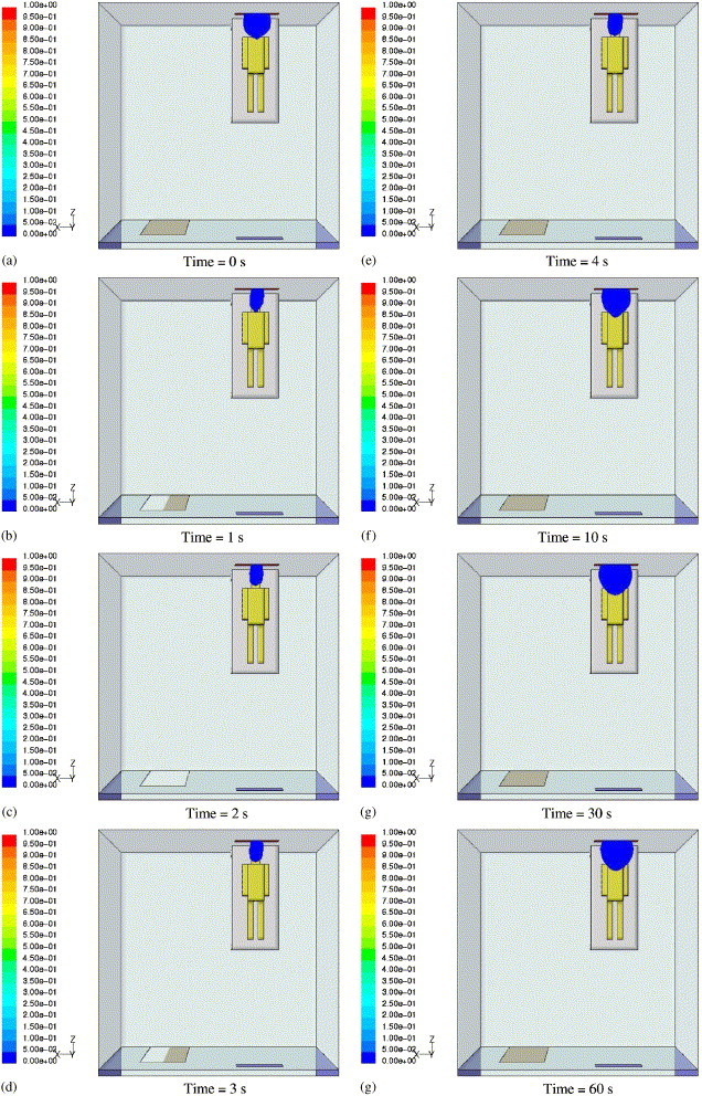
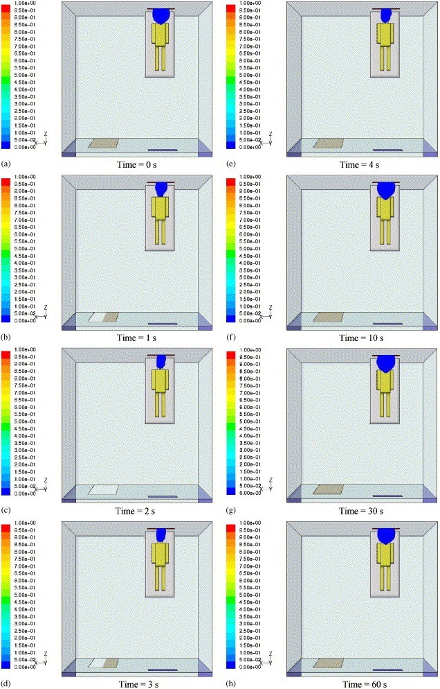
Fig. 2, Fig. 3 show the transient velocity and pressure distributions at the height of 1 m above the floor, under the influence of a moving person moving at different speeds. When the moving speed is equal to 0.25 m/s, transient velocity fields shown in Figs. 2(a) and (b) indicate that the moving person slightly disturbs room air distribution and a weak vortex flow develops behind it. However, Figs. 3(a) and (b) show uniform pressure distribution in this case. When the movement is faster, the variations of velocity and pressure fields become obvious and stronger vortex flow forms behind the moving person, as depicted in other Fig. 2, Fig. 3. Although faster moving speeds result in larger velocity and pressure variations, those changes disappear and the flow field returns to the original state quickly, which usually takes less than 30 s after the moving person returns to the original position. To investigate the contaminant transport affected by the moving person, iso-contours of dimensionless CO2 concentration C d equal to 1/1000 are presented in Figs. 4(a)–(f) . From these figures, it is found that the iso-contour is concentrated only near the mouth of the patient, and not spread out, no matter what the speed of the moving person is. If the standing person remains motionless, the same iso-contours as those of Figs. 4(a)–(f) is displayed in Fig. 5 , revealing that the range of contaminant transport is limited only to the surrounding area of the mouth, similar to those results of Figs. 4(a)–(f). The results shown in Figs. 4(a)–(f) indicate that the contaminant transport from the mouth of the patient is not obviously affected by the speed of the moving person.
Fig. 2.
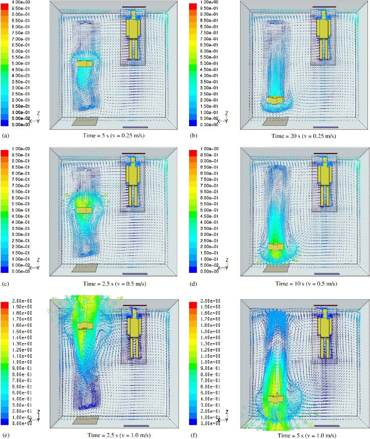
Transient velocity distributions at y=1 m for different speeds of a moving person.
Fig. 3.
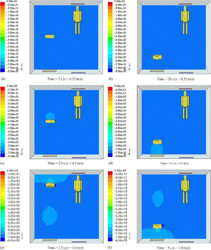
Transient pressure distributions at y=1 m for different speeds of a moving person.
Fig. 4.
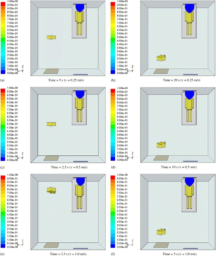
Transient iso-contours of Cd=1/1000 for different speeds of a moving person.
Fig. 5.
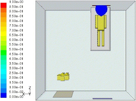
Iso-contour of Cd=1/1000 at steady state for the case of motionless standing person.
3.2. Case B: Effect of movement of the sliding door
To investigate the effect of the movement of the sliding door on room air distribution, the numerical simulation of this case adopts a domain composed of an isolation room and an anteroom, as displayed in Fig. 1(b). The volume of the isolation room is the same as that of the previous case and the anteroom has the volume of 4 m (X)×2.5 m (Y)×1.5 m (Z). Both rooms are connected only by a sliding door with the frontal area of 0.8×2 m2 and the thickness of 0.1 m. Assume that there is no airflow exchange between the two rooms when the sliding door is closed. The static pressure of the anteroom is specified by 0 Pa. Other boundary conditions are the same as those of the previous case. To study the influence of the pressure difference between both rooms on room air distribution, the pressure differences of 2.5 and 8 Pa are used. In order to maintain negative internal pressure within the isolation room, the static pressures of −2.5 and −8 Pa are given at the air outlet, respectively. Each action of opening and closing the door lasts for 2 s and the time duration for one cycle of opening and closing door is 4 s. After one cycle of opening and closing door is completed, the door is closed until the flow field reaches steady state. Grid elements of 76,842 and time step of 0.1 s are adopted in the dynamic analysis.
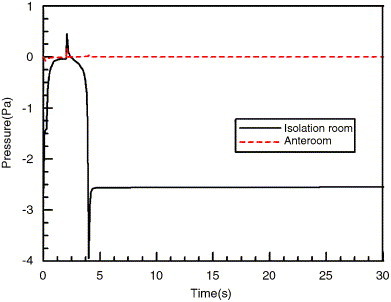
To analyze room pressure distribution affected by different pressure differences between two rooms, Fig. 6, Fig. 7 show that the average static pressures of the isolation room and anteroom vary with time. They indicate that the internal pressure within the isolation room rises suddenly at the instant of opening the door and reaches the pressure of the anteroom after one second of opening the door. Due to the action of opening the door, the negative internal pressure disappears quickly and the pressures of both rooms equate quickly. At the moment of closing the door, the internal pressure of the isolation room suddenly rises to a higher pressure than that of the anteroom. When the door continues to close, the internal pressure drops quickly and becomes negative again. At the instant that the door is closed completely, the internal room pressure is lower than the specified negative internal pressure and it then rises rapidly to achieve the specified negative internal pressure. At the rest time of numerical simulation, the internal room pressure remains constant after it returns to the specified negative internal pressure. From the above discussion, it can be seen that no matter what the specified negative internal pressure is, the transient variations of internal room pressures have the same trends.
Fig. 6.
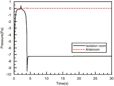
Transient variations of average static pressures of the isolation room and anteroom (ΔP=8 Pa).
Fig. 7.
Transient variations of average static pressures of the isolation room and anteroom (ΔP=2.5 Pa).
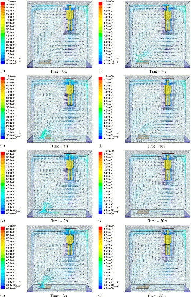
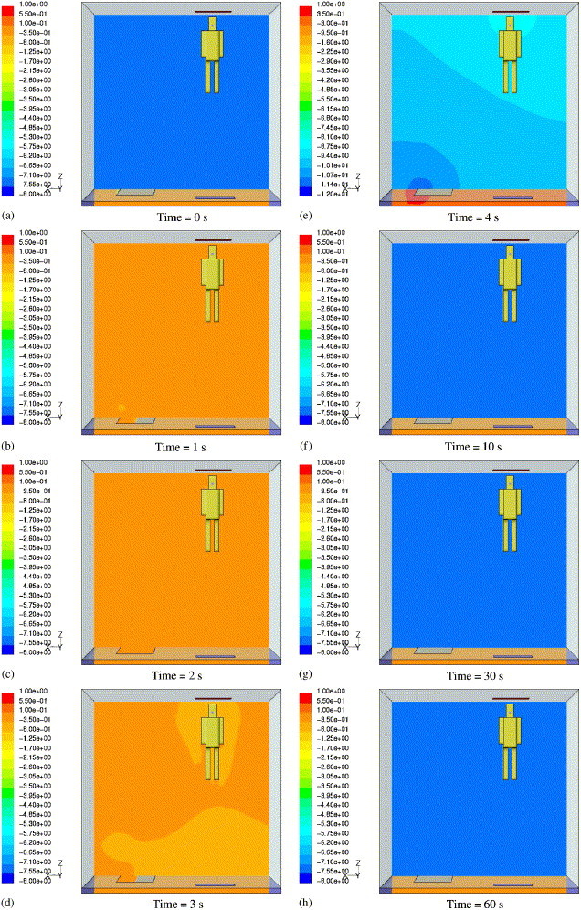
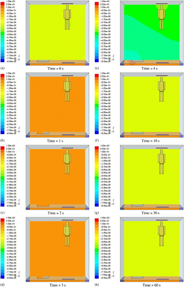
Due to the pressure difference between the two rooms, the airflow enters the isolation room from the anteroom when the door is opened. Transient velocity fields are shown in Fig. 8, Fig. 9 for two kinds of pressure differences between both rooms, showing that larger pressure difference induces more airflow into the isolation room during the period of opening door. Fig. 10, Fig. 11 display the transient pressure distributions for two kinds of specified pressure differences, showing that the results have similar trends as those of Fig. 6, Fig. 7. Because a larger pressure difference causes more airflow into the isolation room, it has a greater effect on removing the contaminant. Therefore, during the period of opening door, the area of iso-contour of for the condition of ΔP=8 Pa is smaller than that of ΔP=2.5 Pa, as shown in Fig. 12, Fig. 13 . However, after the door is closed, the surrounding areas of iso-contours for both kinds of specified pressure differences are almost the same, revealing that the contaminant transport is not affected by the magnitude of the specified pressure difference.
Fig. 8.

Transient velocity distributions at y=1 m for the case of the movement of a sliding door (ΔP=8 Pa).
Fig. 9.
Transient velocity distributions at y=1 m for the case of the movement of a sliding door (ΔP=2.5 Pa).
Fig. 10.
Transient pressure distributions at y=1 m for the case of the movement of a sliding door (ΔP=8 Pa).
Fig. 11.
Transient pressure distributions at y=1 m for the case of the movement of a sliding door (ΔP=2.5 Pa).
Fig. 12.
Transient iso-contours of Cd=1/1000 at y=1 m for the case of the movement of a sliding door (ΔP=8 Pa).
Fig. 13.
Transient iso-contours of Cd=1/1000 at y=1 m for the case of the movement of a sliding door (ΔP=2.5 Pa).
4. Conclusion
In this study, the CFD method has been used to investigate the effects of a moving person and the movement of a sliding door on the air distribution within the isolation room. The following conclusions can be made:
-
(1)
Although the air distribution, including velocity, and pressure fields, is easily affected by the moving person, the disturbed room airflows return to the original state quickly after the walking person returns to the original position and remains motionless. Moreover, the removal of contaminants from the source is not obviously affected by the moving speed.
-
(2)
The opening and closing of a sliding door has profound effects on internal pressure and velocity distributions. It induces airflow into the isolation room from the anteroom and causes sudden rises and drops of the internal pressure during the periods of opening and closing door. Moreover, no matter what the specified pressure difference is, the pressure variations within the isolation room have the same trends. However, contaminant transport is affected only by the magnitude of the specified pressure difference during the period of opening door. After the door is closed, the removal of contaminant source is not influenced by the magnitude of the specified pressure difference.
Acknowledgment
The authors would like to express their gratitude for support from ChiJing Fab Technology Ltd., Taiwan, ROC.
References
- 1.ASHRAE Handbook . American Society of Heating, Refrigeration and Air-Conditioning Engineers, Inc.; USA: 1997. Fundamentals. [PMC free article] [PubMed] [Google Scholar]
- 2.Murakami S., Kaizuka M., Yoshino H., Kato S. American Society of Heating, Refrigeration and Air-Conditioning Engineers, Inc.; USA: 1992. Room air convection and ventilation effectiveness. [Google Scholar]
- 3.Chen Q. Computational fluid dynamics for HVAC: success and failures. ASHRAE Transactions. 1992;103(1):178–187. [Google Scholar]
- 4.Li Y., Baldacchino L. Implementation of some higher-order convection schemes on non-uniform grids. International Journal for Numerical Methods in Fluids. 1995;21:1201–1220. [Google Scholar]
- 5.Murakami S., Kato S., Ooka R. Comparison of numerical predictions of horizontal nonisothermal jet in a room with three turbulence models—k−ε EVM, ASM, and DSM. ASHRAE Transactions. 1994;100(2):697–704. [Google Scholar]
- 6.Neilson P.V. The selection of turbulence models for prediction of room airflow. ASHRAE Transactions. 1998;104(1):1119–1127. [Google Scholar]
- 7.Xu W., Chen Q., Nieuwstadt F.T.M. A new turbulence model for near-wall natural convection. International Journal of Heat and Mass Transfer. 1998;41:3161–3176. [Google Scholar]
- 8.Gan G. Evaluation of room air distribution systems using computational fluid dynamics. Energy and Buildings. 1995;23:83–93. [Google Scholar]
- 9.Gan G., Awbi H.B. Numerical prediction of the age of air in ventilated rooms. ROOMVENT’94. 1994;2:16–27. [Google Scholar]
- 10.Chung I.P., Rankin D. Using numerical simulation to predict ventilation efficiency in a model room. Energy and Buildings. 1998;28:43–50. [Google Scholar]
- 11.Lee H., Awbi H.B. Effect of internal partitioning on indoor air quality of rooms with mixing ventilation-basic study. Building and Environment. 2004;39:127–141. [Google Scholar]
- 12.Hyun S., Kleinstreuer C. Numerical simulation of mixed convection heat and mass transfer in a human inhalation test chamber. International Journal of Heat and Mass Transfer. 2001;44:2247–2260. [Google Scholar]
- 13.Bjørn E., Neilson P.V. Exposure due to interacting air flows between two persons. ROOMVENT’96. 1996;2:107–114. [Google Scholar]
- 14.Matsumoto H. Influence of moving object on air distribution in ventilated rooms. ROOMVENT’2002. 2002;1:261–264. [Google Scholar]
- 15.FLUENT 6.1. User's Guide. FLUENT Inc. 2003.
- 16.Patankar S.V. Hemisphere Publishing Corporation; New York: 1980. Numerical heat transfer and fluid flow. [Google Scholar]