

Abstract
Since it first appeared in China's Guangdong Province, Severe Acute Respiratory Syndrome (SARS) has caused serious damages to many parts of the world, especially Asia. Little is known about its epidemiology. We developed a modified discrete SIR model including susceptible individuals, non-hospitalized SARS persons; hospitalized patients, cured hospital patients, and those who have died due to SARS infection. Here, we demonstrate the effective reproduction number is determined by infection rates and infectious period of hospitalized and non-hospitalized SARS patients. Both infection rate and the effective reproductive number of the SARS virus are significantly negatively correlated with the total number of cumulative cases, indicating that the control measures implemented in China are effective, and the outbreak pattern of accumulative SARS cases in China is a logistic growth curve. We estimate the basic reproduction number R0 of SARS virus is 2.87 in mainland of China, very close to the estimations in Singapore and Hong Kong.
Keywords: Severe Acute Respiratory Syndrome (SARS), Epidemiology, Model, Effective reproduction number
1. Introduction
The first SARS case was reported in China's Guangdong Province in November of 2002. The total number of cases recorded in China climbed to over 5200 with about 5–10% mortality by the end of 2003. It has been confirmed that SARS is caused by a new coronavirus, but its epidemiology is little known (Dye and Gay, 2003, Lipsitch et al., 2003, Riley et al., 2003). Consequently, modelers are struggling to estimate the severity of the SARS epidemic, the effectiveness of control measures and to provide earlier warning of possible SARS outbreaks (Vogel, 2003). Mathematical models have been widely used to calculate and describe the dynamic evolution of epidemic threshold values and severity (Bailei, 1975, Anderson and May, 1992). The most widely used is the Kermarck-McKendrik model, also called the SIR model (Capasso and Serio, 1978), which is based on a system of three populations: susceptible, infectious and removals. Various epidemic models have been developed from the classic SIR model for different purposes, or with different assumptions, e.g. the SIRS model (Mollison, 1995), SEIR model (Keepling et al., 1997), two-level or two-stage SIR model (Ball and Neal, 2002), SIR models considering immunity (Greenhalgh et al., 2000), intermediate class (Méndez and Fort, 2000), non-linearity of infection (Moghadas, 2002, Wendi and Zhien, 2002, Ruan and Wang, 2003), etc. In classic SIR models, the effective reproductive number, R, is the threshold parameter of epidemic diseases: if R < 1, the disease will eventually disappear, but R > 1 implies that the disease will persist (Hethcote and van den Driesssche, 1995, Wallinga et al., 1999, Diekmann et al., 1990). Therefore, knowledge of R is extremely valuable for developing epidemic management strategies as it gives some indication of the effort required to reach specific goals (Wendi and Zhien, 2002, Ruan and Wang, 2003). Recently, two studies reported the transmission epidemic of SARS in Singapore and Hong Kong (Dye and Gay, 2003, Lipsitch et al., 2003, Riley et al., 2003). Both estimated the basic reproduction number R 0 is order of 2–4. Both teams make use of mathematical models based on a system of four subpopulations: susceptible, exposed, infectious, and recovered (immune) individual, also called a SEIR model.
2. The discrete models
We developed a discrete SARS model based on the following groups: susceptible individuals, N 1(t); non-hospitalized SARS persons, N 2(t); hospitalized patients, N 3(t); cured hospital patients, N 4(t); and those who have died due to SARS infection, N 5(t); (Fig. 1a). The infectious period of non-hospitalized patients, T 1(t), is defined as the time non-hospitalized SARS persons from being infectious to being removed to hospitals. We assume that non-hospitalized SARS persons are infectious at the rate P 1(t). Infected people with symptoms, once detected, are removed immediately to hospital for isolation and treatment. These infected patients further infect doctors, nurses and other front-line hospital staff at the rate P 2(t) during the treatment period T 2(t) in hospitals. Non-hospitalized SARS individuals are composed of two sub-groups: front-line hospital staff (doctors, nurses, etc.), N 2d(t), and the general public, N 2n(t). Non-hospitalized SARS people, N 2(t), infect the general public, N 2n(t), at the rate P 1(t), while hospitalized SARS patients, N 3(t), infect front-line hospital staff, N 2d(t), at the rate P 2(t). The transfer rates from N 2(t) to N 3(t) is determined by T 1(t), and the transfer rate from N 3(t) to N 4(t) or N 5(t) are determined by the proportion of cured patients, P 3(t), and T 2(t). The proportion of mortality due to SARS infection is 1 − P 3(t). This model is especially designed for estimating the basic and effective reproductive number of the SARS virus from the data that has been released daily by the Chinese Ministry of Health (CMH) since April 21, 2003.
Fig. 1.

(a) Diagramatic representation of the SARS model. See text for symbol definitions; (b) the outbreak pattern and the effective reproductive number of the SARS model. When R < 1 (○), the outbreak curve is a power curve (P1 = 0.0062, P2 = 0.1473, T1 = 4.5, T2 = 14); when R > 1(□), the outbreak curve is exponential (P1 = 0.0378, P2 = 0.2144, T1 = 4.5, T2 = 14); when R = 1(▴), the outbreak curve is linear (P1 = 0.01404, P2 = 0.1785, T1 = 4.5, T2 = 14). The initial values of total cumulative cases, cumulative mortality, cumulative recovered patients and cumulative cases are 3106, 139, 1306 and 653, respectively.
We assume that the immigration and emigration rates of infected individuals are the same. Clinical observations indicate that cured SARS patients are unlikely to be infectious again (Yang, 2003). We will ignore the effect of natural birth and mortality rates because we are only interested in the dynamics of the SARS epidemic over a period of short time (e.g. a few weeks or months). The dynamic model is described as below:
| (1) |
| (2) |
| (3) |
| (4) |
| (5) |
Notice that, P 1(t)·N 2(t) is the number of new SARS cases among the general public caused by N 2(t); and P 2(t)·N 3(t) is the number of new SARS cases among front-line hospital staff caused by N 3(t). We assume the T 1(t) of N 2n(t) and N 2d(t) is same, then:
| (6) |
| (7) |
The time step in our models is set as one day.
3. Theoretical analysis
First, let us assume that the growth pattern of total cumulative SARS cases is linear against time t, and let N s(t) be total cumulative SARS cases at time t, then:
Here, b 0, b 1 are constants.
b 1 is the number of new SARS cases at time t. That is to say, if b 1 is constant, the growth pattern of SARS cases is linear against time t. From Eq. (3), the number of new cases of SARS removed to N 3(t) is N 2(t)/T 1(t), then N s(t + 1) − N s(t) = N 2(t)/T 1(t). If N 2(t + 1) − N 2(t) = 0, N s(t + 1) − N s(t) is constant and the growth pattern of SARS cases will be linear; if N 2(t + 1) − N 2(t) > 0 it will be exponential; if N 2(t + 1) − N 2(t) < 0 it will be a power curve. From Eq. (2):
| (8) |
For a linear growth pattern N 2(t) has to be stable. To satisfy the Eq. (8), N 3(t) also has to be stable: N 3(t + 1) − N 3(t) = 0. From Eq. (3):
If N 3(t + 1) − N 3(t) = 0, N 3(t)/N 2(t) = T 2(t)/T 1(t). From Eq. (8), then
| (9) |
Let R(t) = P 1(t)·T 1(t) + P 2(t)·T 2(t), the outbreak pattern of SARS cases is determined by the following conditions: R(t) = 1, linear growth; R(t) > 1, exponential growth; R(t) < 1, power growth. If P 2(t) = 0, i.e. SARS infection among front-line hospital staff is completely controlled, then the Eq. (9) is written as: R(t) = P 1(t)·T 1(t) = 1. Through qualitative analysis, we conclude that the outbreak pattern of SARS cases is determined by four parameters: the infection rate among the general public P 1(t) and front-line hospital staff P 2(t), the infectious period of non-hospitalized patients T 1(t) and the treatment period of SARS patients in hospital T 2(t).
4. Model parameter estimation
The data provided by the CMH include total cumulative SARS cases, cumulative SARS cases among front-line hospital staff, cumulative SARS mortality, cumulative cured SARS cases, and cumulative suspected SARS cases on the Chinese Mainland (Table 1 ). Let us define:
N s(t) is total cumulative SARS cases at time t;
N d(t), cumulative SARS cases among front-line hospital staff at time t;
N n(t), cumulative SARS cases among general public at time t;
N 5(t) is cumulative SARS mortality at time t;
N 4(t) is cumulative cured SARS cases at time t.
Then:
| (10) |
| (11) |
| (12) |
| (13) |
| (14) |
| (15) |
| (16) |
The weekly average values of P 1(t), P 2(t) last week at time t are calculated as:
| (17) |
| (18) |
The standard errors were estimated by following Krebs (1999). Let p 1 = P 1_w(t); q 1 = 1 − p 1; ; p 2 = P 2_w(t); q 2 = 1 − p 2; ; S 1, S 2 and S are standard errors of P 1_w(t), P 2_w(t) and R(t), then:
It is obvious that using the rolling weekly averages of infection rates reduces estimation errors since the higher the , the lower the standard errors.
Table 1.
The cumulative SARS cases in Mainland China from April 21 to May 12, 2003, released by the Chinese Ministry of Health
| Date | Days | Total | Dead | Cured | Doctorsa |
|---|---|---|---|---|---|
| April 21 | 1 | 2158 | 97 | 1213 | 480 |
| April 22 | 2 | 2305 | 106 | 1231 | 517 |
| April 23 | 3 | 2422 | 110 | 1254 | 541 |
| April 24 | 4 | 2601 | 115 | 1277 | 578 |
| April 26 | 6 | 2753 | 122 | 1285 | 588 |
| April 27 | 7 | 2914 | 131 | 1299 | 610 |
| April 28 | 8 | 3106 | 139 | 1306 | 653 |
| April 29 | 9 | 3303 | 148 | 1322 | 709 |
| April 30 | 10 | 3460 | 159 | 1332 | 727 |
| May 1 | 11 | 3638 | 181 | 1351 | 753 |
| May 2 | 12 | 3799 | 322 | 1372 | 778 |
| May 3 | 13 | 3971 | 190 | 1406 | 810 |
| May 4 | 14 | 4125 | 197 | 1416 | 832 |
| May 5 | 15 | 4280 | 206 | 1433 | 851 |
| May 6 | 16 | 4409 | 214 | 1460 | 883 |
| May 7 | 17 | 4560 | 219 | 1487 | 901 |
| May 8 | 18 | 4698 | 224 | 1529 | 917 |
| May 9 | 19 | 4805 | 230 | 1582 | 925 |
| May 10 | 20 | 4884 | 235 | 1620 | 931 |
| May 11 | 21 | 4948 | 240 | 1652 | 935 |
| May 12 | 22 | 5013 | 252 | 1693 | 941 |
Source: Chinese Ministry of Health.
Includes all front-line hospital staff.
Clinical observations indicate that in mainland of China, the infectious period of the non-hospitalized persons is usually between 4 and 5 days with an average of 4.5 days (Yang, 2003). The average treatment period (admission to discharge) of hospitalized SARS patients is 14 days. About 95% of patients are completely cured. Thus, we assume that the parameters of T 1(t), T 2(t) and P 3(t) are constant, and let T 1 = 4.5, T 2 = 14, P 3 = 0.95. The model parameters P 1_w(t), P 2_w(t), R(t), and their standard errors are shown in Table 2 .
Table 2.
Estimated values of P1_w(t), P2_w(t), R(t) and their standard errors S1, S2 and S
| Date | Day | Ns | r | P2_w(t) | S2 | P1_w(t) | S1 | R(t) | S | ||
|---|---|---|---|---|---|---|---|---|---|---|---|
| April 21 | 1 | 2158 | 0.0659 | ||||||||
| April 22 | 2 | 2305 | 0.0495 | ||||||||
| April 23 | 3 | 2422 | 0.0713 | ||||||||
| April 24 | 4 | 2601 | 0.0568 | ||||||||
| April 26 | 6 | 2753 | 0.0568 | ||||||||
| April 27 | 7 | 2914 | 0.0638 | 6841 | 0.0378 | 0.0023 | 4266 | 0.2144 | 0.0063 | 1.4937 | 0.0159 |
| April 28 | 8 | 3106 | 0.0615 | 8502 | 0.0169 | 0.0014 | 5152.5 | 0.2031 | 0.006 | 1.1503 | 0.0130 |
| April 29 | 9 | 3303 | 0.0464 | 9505 | 0.0230 | 0.0015 | 5197.5 | 0.2329 | 0.0059 | 1.3706 | 0.0137 |
| April 30 | 10 | 3460 | 0.0502 | 10506 | 0.0150 | 0.0012 | 5472 | 0.1786 | 0.0052 | 1.014 | 0.0118 |
| May 1 | 11 | 3638 | 0.0433 | 11565 | 0.0259 | 0.0015 | 5391 | 0.1835 | 0.0053 | 1.1875 | 0.0125 |
| May 2 | 12 | 3799 | 0.0443 | 12461 | 0.0178 | 0.0012 | 5481 | 0.1760 | 0.0051 | 1.0413 | 0.0118 |
| May 3 | 13 | 3971 | 0.0381 | 13490 | 0.0085 | 0.0008 | 5449.5 | 0.1708 | 0.0051 | 0.8867 | 0.0112 |
| May 4 | 14 | 4125 | 0.0369 | 14572 | 0.0062 | 0.0007 | 5283 | 0.1473 | 0.0049 | 0.7492 | 0.0106 |
| May 5 | 15 | 4280 | 0.0297 | 15552 | 0.0112 | 0.0008 | 4977 | 0.1818 | 0.0055 | 0.9749 | 0.0120 |
| May 6 | 16 | 4409 | 0.0337 | 16454 | 0.0078 | 0.0007 | 4950 | 0.1598 | 0.0052 | 0.8289 | 0.0113 |
| May 7 | 17 | 4560 | 0.0298 | 17339 | 0.0051 | 0.0005 | 4770 | 0.1529 | 0.0052 | 0.7589 | 0.0112 |
| May 8 | 18 | 4698 | 0.0225 | 18167 | 0.0017 | 0.0003 | 4527 | 0.1232 | 0.0049 | 0.5773 | 0.0104 |
| May 9 | 19 | 4805 | 0.0163 | 19055 | 0.0021 | 0.0003 | 4108.5 | 0.1139 | 0.0050 | 0.542 | 0.0106 |
| May 10 | 20 | 4884 | 0.0130 | 19709 | 0.0023 | 0.0003 | 3703.5 | 0.1009 | 0.0050 | 0.4854 | 0.0106 |
| May 11 | 21 | 4948 | 0.0131 | 20253 | −0.002 | – | 3298.5 | 0.1608 | 0.0064 | 0.6895 | – |
| May 12 | 22 | 5013 | 0.0145 | 20680 | 0.0000 | 3.4E−05 | 3046.5 | 0.0552 | 0.0041 | 0.2485 | 0.0088 |
Ns is the total cumulative SARS cases. r is the instantaneous increase rate. “–” S2 and S are not calculated due to the negative value of P2(t).
The instantaneous rate of increase in cumulative SARS cases N s(t) is defined as: r = ln[N s(t + 1)/N s(t)]. If the instantaneous rate of increase is negative and linear correlated with cumulative SARS cases, the growth pattern of cumulative SARS cases is a logistic (Zhang et al., 2003).
5. Results
Fig. 1b illustrates how effective reproductive number R determines the outbreak pattern of SARS cases. The initial values of N 1(0), N 2(0), N 3(0), N 4(0), N 5(0) are from the data of April 21, 2003, released by CMH. Changing the values P 1, P 2, P 3, T 1 and T 2 produce different curves for the total number of cumulative cases. The simulation results further support the conclusion that R is the threshold for the outbreak pattern of SARS.
Sensitivity analysis indicates that T 1 and P 1 are the most sensitive parameters, T 2 and P 2 are less sensitive and P 3 is the least sensitive (Fig. 2 ). Therefore, R is mainly determined by P 1, P 2, T 1 and T 2.
Fig. 2.
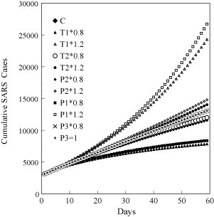
Sensitivity analysis of model parameters P1, P2, P3, T1, T2. Each parameter was increased or reduced by 20% while the other parameters remained unchanged. The linear curve is the contrasting curve (C) (R = 1, P1 = 0.01404, P2 = 0.1785, T1 = 4.5, T2 = 14). The initial values of total cumulative cases, cumulative mortality, cumulative recovered patients and cumulative cases are 3106, 139, 1306 and 653, respectively. The curves of P3* 1.2 and P3* 0.8 are totally overlapped with the contrasting curve (C).
Fig. 3a shows that the effective reproductive number (R) and infection rates (P 1, P 2) among front-line hospital staff and the general public are significantly negatively correlated with total cumulative SARS cases (N s). The instantaneous rate of increase in total cumulative cases is also significantly negatively correlated with the number of total cumulative cases, indicating that the outbreak pattern of cumulative SARS cases in China is a logistic growth curve. Table 3 shows the results of linear regression between dependents variables (R, P 2, P 1, r) and independent variable (N s). From Table 3, the maximum R (equal basic reproductive number R 0), P 2, P 1, r (equal b 0 in Table 3) are 2.8716, 0.0684, 0.4245 and 0.1129 when the cumulative SARS case (N s) is approaching zero. Therefore, in the early stage of SARS outbreak, each SARS infect 1.9 (P 1·T 1 = 0.4245 × 4.5) members of the general public, 0.9576 (P 2·T 2 = 0.0684 × 14) front-line hospital staff. During the study period, we estimate that each infected individual infects 0.48–1.49 individuals, average 0.93 (0.18 front-line hospital staff and 0.75 members of the general public) during the study period of 3 weeks. In general, the infection of SARS person to front-line hospital staff is better managed due to the improved protection measures taken in hospitals.
Fig. 3.

(a) The negative relationship between the SARS infection rate among the general public (P1, ▴) (R2 = 0.743, p = 0.000), the infection rate among front-line hospital staff (P2, +) (R2 = 0.740, p = 0.000), the effective reproductive number (R, ×) (R2 = 0.813, p = 0.000), the relative rate of increase of total cumulative cases (r, ●) (R2 = 0.934, p = 0.000) against total cumulative cases of SARS in China. (b) The simulated total cumulative SARS cases (Ns − S, +), observed values of the total cumulative SARS cases (Ns − O, ■), the simulated cumulative SARS cases among front-line hospital staff (Nd − S, ×), the observed cumulative SARS cases among front-line hospital staff (Nd − O, ▴), the simulated cumulative SARS cases among the general public (Nn − S, *) and the observed cumulative SARS cases among the general public (Nd − O, ●) in China from April 21 to May 12, 2003.
Table 3.
Linear regressions between dependents (R, P2, P1, r) and independent Ns by using linear models: r = b0 + b1Ns, R = b0 + b1Ns, P2 = b0 + b1Ns, P1 = b0 + b1Ns
| Dependent | Mth | R2 | d.f. | F | Sigf | b0 | b1 |
|---|---|---|---|---|---|---|---|
| R | LIN | 0.875 | 16 | 111.80 | 0.000 | 2.8716 | −0.0005 |
| P2 | LIN | 0.833 | 16 | 79.57 | 0.000 | 0.0684 | −0.00001 |
| P1 | LIN | 0.745 | 16 | 46.83 | 0.000 | 0.4245 | −0.00007 |
| r | LIN | 0.909 | 22 | 218.51 | 0.000 | 0.1129 | 0.00002 |
Fig. 3b shows the simulated and observed values of total cumulative cases, cumulative cases among front-line hospital staff and the general public. The negative relationship between infection rates and cumulative cases has been incorporated into the model. In general, the simulation curves are a good fit to the observed growth patterns, but the discrepancy between observed and expected became a little larger over the last week. Higher accuracy of simulation is achieved if it is conducted within a 1-week time frame (Fig. 4 ). These results indicate that the model is generally a good predictor of the dynamics of SARS epidemic.
Fig. 4.

Simulations conducted within a 1-week time frame with the simulated total cumulative SARS cases (+), the simulated cumulative SARS cases among front-line hospital staff (×), the simulated cumulative SARS cases among the general public (*); the observed values of the total cumulative SARS cases (■), the observed cumulative SARS cases among front-line hospital staff (▴), and the observed cumulative SARS cases among the general public (●) in China from April 21 to May 12, 2003. (a) First week, (b) Second week and (c) Third week.
6. Discussions
Although there have been no reported cases of transmission of SARS during pre-symptomatic period (Lipsitch et al., 2003), our study suggests that such transmission by SARS person before hospitalized is quite high; about 2–4 times higher than transmission from hospitalized patients. At present, the transmission process by non-hospitalized persons is not completely understood. Infection paths of nearly 20–30% SARS patients are not clear in mainland of China. Though it is generally believed SARS persons are only infectious during the few days with symptoms, alternative infection paths may exist. According to a survey in China, the SARS virus can survive several days outside the body of SARS persons. It is possible these viruses explain the high proportion of SARS cases without unknown origins.
We estimate that the basic reproductive number R 0 for a single infected individual in the early stage is 2.8716, which is very close to the estimation of R 0 in Singapore and Hong Kong by Lipsitch et al. (2003) and Riley et al. (2003). The rate of SARS transmission is not very high compared to some airborne diseases, which suggests that transmission of the SARS virus requires a relatively long-term period of close contact. This is supported by the fact that SARS cases most often occur among family members, residents or workers in the same apartment complex or office building and front-line hospital staff.
Some epidemiologists have suggested that the apparently linear growth in SARS cases is due to the slow rate of transmission of the virus, and estimate that each infected individual infects no more than two other people (Vogel, 2003). Our study generally supports this speculation, but indicates that the outbreak pattern of the accumulative SARS cases in China is logistic in general, rather than linear. The infection rates, effective reproductive number and the instantaneous rate of increase in total cumulative cases are significantly negatively correlated with the total number of cumulative cases. This is a good indication that the SARS epidemic can be well managed by using traditional prevention measures like isolation, reduction of contacts, etc.
The basic and effective reproductive numbers are good indicators of the severity of epidemic diseases and effectiveness of control (Hethcote and van den Driesssche, 1995). In general, estimation of these parameters from disease outbreak data is not easy since the actual process of infection is not observed, data are often incomplete and the rate of infection is often non-linear. Kramer (1994) accurately simulated the growth of an HIV infected population. Some other methods are also proposed to estimate model parameters, like the Martingale method (Fine and Clarkson, 1982, Yip, 1989, Becker, 1989, Becker, 1993, Haydon et al., 1997, Becker and Britton, 1999), Markov Chain Monte Carlo method (O’Neill, 2002). The SARS model described here is a variant of the SIR model with the addition of two-stage infections and two sub-compartments that reflect unique features of the SARS virus. The model has the advantage that its parameters are easy to estimate from the data released by the CHM. The advantage of our estimation is that R 0, R, P 1, P 2 can be estimated by using simple data of cumulative SARS cases as shown in Table 1.
Our model also includes three basic components: susceptible (N 1), infectious (N 2, N 3) and removals (N 4, N 5). Thus, it is basically a SIR model used widely in epidemiological studies (e.g. Capasso and Serio, 1978, Mollison, 1995, Keepling et al., 1997, Ball and Neal, 2002, Greenhalgh et al., 2000, Dye and Gay, 2003, Lipsitch et al., 2003, Riley et al., 2003). The difference of our model from the classic SIR model is that we further divide the infectious component into two parts: hospitalized and non-hospitalized populations, and we divide the removal component into two parts: cured and dead populations. These modifications were specially done for SARS transmissions. The other difference is that we define the infectious rate differently. Let S(t) is the number of susceptible population at time t, I(t) is the number of infectious population at time t, α is the maximum infection rate, τ is the incubation time. In the classic SIR model (e.g. Monteriro et al., 2006a, Monteriro et al., 2006b), the contribution of I(t) to the increase of newly infection population is calculated as: Δ = α·S(t)·I(t − τ). In our model, we define P(t) as the infection rate of infectious individual of I(t) at time t. Thus, we have the following equation: Δ = P(t)·I(t). The parameter P(t) varies in time. It contains the combined effect of incubation time, immunity and control efforts. In the classic SIR model, α is assumed to be constant, only S(t) and I(t − τ) determine the increase of newly infected population. In fact, isolation measures by human obviously affect the infection rate α. Such an effect is not well presented in the classic SIR model.
It is obvious that our model has advantages over the conventional SIR model because it has fewer parameters. This will make parameter estimation easier without knowing detailed mechanism of disease transmission (e.g. incubation time, immunity and control efforts) and the susceptible population size. Although the parameters of P 1(t), P 2(t), T 1(t), T 2(t) vary in time, it is reasonable to assume they are stable when they are estimated at the rolling interval of 1 week.
Using our model, the infection rate of one infectious individual can easily be estimated at any time if the accumulative numbers of infection and dead cases are given. Though this epidemiological model and the parameter estimation method are specially designed for SARS transmission, they are also applicable to other infectious diseases, and to population growth of other organisms.
The decline of the effective reproductive number indicates that the measures adopted to control SARS in China are effective. One of the key preventative measures in China is the complete isolation of those confirmed or suspected of having been infected, including anyone likely to have had close contact with confirmed or suspected SARS carriers. This measure is strongly recommended because the model shows that both the infectious period (T 1) and the infection rate (P 1) are very sensitive parameters. In addition to isolating confirmed cases reducing the infectious period (T 1) is an effective means of reducing SARS infection. This requires the early identification of infected individuals using modern diagnostic techniques.
Acknowledgements
The study is supported by the Innovation Program of the Chinese Academy of Sciences. I thank Dr. R.J. Moorhouse for their valuable comments and improvements of English writings to this manuscript.
References
- Anderson R.M., May R.M. Oxford University Press; Oxford: 1992. Infectious Diseases of Humans: Dynamics and Control. [Google Scholar]
- Bailei N.T.T. second ed. Griffin; London: 1975. The Mathematical Theory of Diseases. [Google Scholar]
- Ball F., Neal P. A general model for stochastic SIR epidemics with two level of mixing. Math. Biosci. 2002;180:73–102. doi: 10.1016/s0025-5564(02)00125-6. [DOI] [PubMed] [Google Scholar]
- Becker N.G. Parametric inference for epidemic models. Math. Biosci. 1993;117:239–251. doi: 10.1016/0025-5564(93)90026-7. [DOI] [PubMed] [Google Scholar]
- Becker N.G. Chapman and Hall; London: 1989. Analysis of Infectious Disease Data. [Google Scholar]
- Becker N.G., Britton T. Statistical studies of infectious disease incidence. Stat. Soc. Ser. B. 1999;61:287–292. [Google Scholar]
- Capasso V., Serio G. A generalization of the Kermack-McKendrick deterministic epidemic model. Math. Biosci. 1978;42:43–61. [Google Scholar]
- Diekmann O., Heesterbeek H., Metz J.A.J. On the definition and computation of the basic reproductive ratio R0 in the models for infectious diseases in the heterogeneous populations. J. Math. Biol. 1990;28:65–382. doi: 10.1007/BF00178324. [DOI] [PubMed] [Google Scholar]
- Dye C., Gay N. Modeling the SARS epidemic. Science. 2003;300:1884–1885. doi: 10.1126/science.1086925. [DOI] [PubMed] [Google Scholar]
- Fine P.E.M., Clarkson J.A. Measles in England and Wales—I: an analysis of factors underlying seasonal patterns. Int. J. Epidemiol. 1982;11:5–15. doi: 10.1093/ije/11.1.5. [DOI] [PubMed] [Google Scholar]
- Greenhalgh D., Diekmann O., de Jong M.C.M. Subcritical endemic steady states in mathematical models for animal infectious with incomplete immunity. Math. Biosci. 2000;165:1–25. doi: 10.1016/s0025-5564(00)00012-2. [DOI] [PubMed] [Google Scholar]
- Haydon D.T., Woolhouse M.E.J., Kitching R.P. An analysis of foot and mouth disease epidemics in the UK. IMA J. Math. Appl. Med. Biol. 1997;14:1–9. [PubMed] [Google Scholar]
- Hethcote H.W., van den Driesssche P. An SIS epidemic model with variable population size and a delay. J. Math. Biol. 1995;54:177–194. doi: 10.1007/BF00178772. [DOI] [PubMed] [Google Scholar]
- Keepling M.J., Rand D.A., Morris A.J. Correlation models for childhood epidemics. Proc. R. Soc. Lond. 1997;264:1149. doi: 10.1098/rspb.1997.0159. [DOI] [PMC free article] [PubMed] [Google Scholar]
- Kramer I. Accurately simulating the growth in the size of the HIV infected population in AIDS epidemic country: computing the USA HIV infection curve. Math. Comput. Model. 1994;19:91–112. [Google Scholar]
- Krebs C.J. second ed. Addision-Welsey Education Publishers, Inc.; 1999. Ecological Methodology. [Google Scholar]
- Lipsitch M. Transmission dynamics and control of severe acute respiratory syndrome. Science. 2003;300:1966–1970. doi: 10.1126/science.1086616. [DOI] [PMC free article] [PubMed] [Google Scholar]
- Méndez V.M., Fort J. Dynamical evolution of discrete epidemic models. Physica A: Statist. Mech. Appl. 2000;284:309–317. [Google Scholar]
- Moghadas S.M. Global stability of two-stage epidemic model with generalized non-linear incidence. Math. Comput. Simulat. 2002;60:107–118. [Google Scholar]
- Mollison D. Cambridge University Press; Cambridge: 1995. Epidemic Models: Their Structure and Relation to Data. [Google Scholar]
- Monteriro L.H.A., Chimara H.D.B., Beilinck J.G.C. Big cities: shelters for contagious diseases. Ecol. Model. 2006;197:258–262. [Google Scholar]
- Monteriro, L.H.A., Sasso, J.B., Beilinck J.G.C., 2006b. Continous and discrete approached to the epidemiology of viral spreading in populations taking into account the delay of incubation time. Ecol. Model., doi:10.1016/j.ecomodel.2006.09.27.
- O’Neill P.D. A tutorial introduction to Bayesian inference for stochastic epidemic models using Markov Chain Monte Carlo methods. Math. Biosci. 2002;180:103–114. doi: 10.1016/s0025-5564(02)00109-8. [DOI] [PubMed] [Google Scholar]
- Riley S. Transmission dynamics of the etiological agent of SARS in Hong Kong: impact of public health interventions. Science. 2003;300:1961–1966. doi: 10.1126/science.1086478. [DOI] [PubMed] [Google Scholar]
- Ruan S., Wang W. Dynamical behavior of an epidemic model with a nonlinear incidence rate. J. Differential Equat. 2003;188:135–163. [Google Scholar]
- Vogel G. Modelers struggle to grasp epidemic's potential scope. Science. 2003;300:558–559. doi: 10.1126/science.300.5619.558. [DOI] [PubMed] [Google Scholar]
- Wallinga J., Edmunds W.J., Kretzchmar M. Perspective: human contact patterns and the spread of airborne infection disease. Trends Microbiol. 1999;9:372–377. doi: 10.1016/s0966-842x(99)01546-2. [DOI] [PubMed] [Google Scholar]
- Wendi W., Zhien M. Global dynamics of an epidemic model with time delay. Nonlinear Anal.: Real World Appl. 2002;3:365–373. [Google Scholar]
- Yang H.M. Science Press; Beijing: 2003. SARS Control Manual. (in Chinese) [Google Scholar]
- Yip P. Estimating the initial relative infection rate for a stochastic epidemic model. Theor. Populat. Biol. 1989;36:202–213. doi: 10.1016/0040-5809(89)90030-0. [DOI] [PubMed] [Google Scholar]
- Zhang Z., Pech R., Davis S., Shi D., Wan X., Zhong W. Extrinsic and intrinsic factors determine the eruptive dynamics of Brandt's voles Microtus brandti in Inner Mongolia, China. Oikos. 2003;100:299–310. [Google Scholar]