Optimal control analysis of a tuberculosis model

Highlights

• •A new TB model with the 4-order cost function is introduced and investigated.
• •The method for the proof of uniqueness of optimal control for the model is new.
• •The numerical results show that the model considered in this paper are effective.

Abstract

In this paper, we extend the model of Liu and Zhang (Math Comput Model 54:836-845, 2011) by incorporating three control terms and apply optimal control theory to the resulting model. Optimal control strategies are proposed to minimize both the disease burden and the intervention cost. We prove the existence and uniqueness of optimal control paths and obtain these optimal paths analytically using Pontryagin’s Maximum Principle. We analyse our results numerically to compare various strategies of proposed controls. It is observed that implementation of three controls is most effective and less expensive among all the strategies. Thus, we conclude that in order to reduce tuberculosis threat all the three controls must be taken into consideration concurrently.

1. Introduction

Tuberculosis (TB) is a major global health threat caused by Mycobacterium tuberculosis (Mtb) that most often affects the lungs (pulmonary TB) but can affect other sites as well (extrapulmonary TB). Fortunately, TB is a preventable and curable disease. Following the World Health Organization (WHO), more than 51 million patients have been successfully treated in countries that adopted the WHO strategy since 1995 [1]. However, the global burden of TB remains enormous. In 2011, there were an estimated 8.7 million new cases of TB (13% co-infected with HIV) and 1.4 million people died from TB [1]. In 2013, there were 9 million new TB cases and 1.5 million TB deaths (in which 0.4 million are HIV-positive patients) [2]. The increase of new cases lies in multiple factors such as the spread of HIV, the collapse of public health programs, the emergence of drug-resistant strains of Mtb [3], [4], [5] and exogenous re-infections, where a latently-infected individual acquires a new infection from another infectious individual (see, for example, [6], [7] and references therein). The TB control approach is the chemoprophylaxis treatment in the absence of an effective vaccine. Neglecting the compliance with drug treatments might result in a relapse and antibiotic resistant TB, i.e. multidrug-resistant TB (MDR-TB) [8]. MDR-TB is one of the most serious health problems and the progress in curing that is slow. Critical funding gaps for TB care and control make it difficult to sustain recent gains, promote further research and develop new drugs and vaccines [1].

It is well known that the mathematical models play vital roles in the dynamics and control of many epidemics including malaria, severe acute respiratory syndromes (SARS) and TB (see, for example, [9], [10], [11], [12], [13], [14], [15], [16], [17] and references therein). Many mathematical dynamic models for TB have been studied extensively in the literature; for instance we refer the reader to [18], [19], [20], [21], [22], [23]. “Fast progressors” and “slow progressors” are two different ways considered by most models to progress to active disease after infection. The probability of latent and treated individuals who might be reinfected [24] is also taken into account by some latest models as the infection and/or disease do not confer full protection which is already well recognized [25]. Some previous models of TB, especially the predictive models endeavor to calculate a threshold called basic reproductive number. The dynamics of transmission of the disease has been analyzed in terms of the reduction of the basic reproductive number. Since the first paper published by Jung et al. [8] in 2002, the time dependent optimal control strategies have been employed in the study of dynamics of TB mathematical models by many authors (see, for example, [8], [26], [27], [28], [29], [30], [31], [32], [33], [34]). Valuable theoretical results generated by both approaches of studying control strategies can be used to guide epidemic control programs. Various objective criteria may be adopted, according to a chosen goal (or goals).

In 2011, considering that the treated individuals are also infectious, Liu and Zhang [24] proposed a nonlinear TB model system as follows:

$$\begin{array}{c}\hfill \{\begin{array}{c}\frac{dS}{dt}=\Lambda -\beta S(I+{\rho }_{1}T)-(\mu +p)S,\hfill \\ \frac{dV}{dt}=pS-{\rho }_2\beta V(I+{\rho }_{1}T)-\mu V,\hfill \\ \frac{dL}{dt}=l\beta S(I+{\rho }_{1}T)+{\rho }_2\beta V(I+{\rho }_{1}T)-(\mu +\delta )L+\rho T,\hfill \\ \frac{dI}{dt}=(1-l)\beta S(I+{\rho }_{1}T)+\delta L-(\mu +\alpha +\gamma )I,\hfill \\ \frac{dT}{dt}=\gamma I-(\mu +\rho )T,\hfill \\ N\left(t\right)=S\left(t\right)+V\left(t\right)+L\left(t\right)+I\left(t\right)+T\left(t\right),\hfill \end{array}\end{array}$$ (1.1)

where a population of size N(t) is partitioned into five subclasses: susceptible (S(t)), vaccinated (V(t)), individuals infected with TB in latent stage (L(t)), individuals infected with TB in the active stage (I(t)) and treated individuals infected with TB (T(t)). The parameter Λ represents the constant recruitment rate of susceptible individuals. Parameter p is the rate at which susceptible individuals are moved into the vaccination process. The natural death rate is µ. The disease-induced death rate coefficient for individuals in compartment I is α. Parameter ρ represents the rate that individuals successfully treated of TB return to the latent TB stage and parameter γ is the treatment rate in the infective class. It is assumed that the time before latent individuals become infectious obeys an exponential distribution, with mean waiting time $\frac{1}{\delta }$. Thus, δ is the rate at which an individual leaves the latent compartment to become infectious. Susceptible individuals acquire TB infection from individuals with active TB at rate $\beta S(I+{\rho }_{1}T),$ where β is the disease transmission coefficient, and the parameter ρ ₁ < 1 accounts for the reduction in infectiousness among individuals with active TB who are treated (in comparison to those who are not treated). Fraction l of susceptible individuals who acquire TB infection is assumed to enter the latent TB class (L), at the rate $\beta S(I+{\rho }_{1}T),$ while the remainder moves to the active TB class (I). It is assumed that individuals in the latent class do not transmit infection. The vaccinated individuals are infected at rate ${\rho }_2\beta V(I+{\rho }_{1}T),$ where ρ ₂ < 1 represents the reduction in risk of infection owing to vaccination (for a vaccine that offers 100% protection, ${\rho }_2=0$; thus in reality 0 < ρ ₂ < 1). For model (1.1), Liu and Zhang [24] first obtained the basic reproduction number

$$\begin{array}{c}\hfill R_0=\frac{(\mu +\rho +\gamma {\rho }_1)(\beta \delta {\rho }_2{V}^0+\beta \delta S^0+\beta \mu (1-l)S^0)}{(\mu +\delta )(\mu +\rho )(\mu +\alpha +\gamma )-\delta \rho \gamma },\end{array}$$

where

$$\begin{array}{c}\hfill S^0=\frac{\Lambda }{\mu +p},V^0=\frac{\Lambda p}{\mu (\mu +p)}.\end{array}$$

After that they showed that if the basic reproduction number R ₀ of the model system is below one then disease dies out otherwise it persists. This indicates that the basic reproduction number, R ₀, plays a crucial role in characterizing dynamics of the disease and could be used to suggest or design TB control strategies. However, they did not further investigate time dependent control strategies since their discussions had been concentrated on prevalence of TB at equilibria. Note that, for system (1.1), ρ represents successful treatment rate. Computing the partial derivative of R ₀ with respect to ρ gives that $\frac{\partial R_0}{\partial \rho }{|}_{\left(1.1\right)}<0$ if ${\rho }_1>\frac{\mu \delta }{(\mu +\delta )(\mu +\alpha )+\mu \gamma }$. Therefore, improving successful treatment rate helps to reduce TB infection when ${\rho }_1>\frac{\mu \delta }{(\mu +\delta )(\mu +\alpha )+\mu \gamma }$. Using the fact that $\frac{\partial R_0}{\partial \gamma }{|}_{\left(1.1\right)}<0$ as long as ${\rho }_1<\frac{\mu (\mu +\rho +\delta )}{(\mu +\delta )(\mu +\alpha )},$ Liu and Zhang [24] pointed out that the treatment of TB-infected individuals in the active stage would have positive impact if ${\rho }_1<\frac{\mu (\mu +\rho +\delta )}{(\mu +\delta )(\mu +\alpha )}$. In other words, if ρ ₁ lies between two certain thresholds, then increasing ρ and γ have positive meaning on controlling TB infection. Furthermore, $\frac{\partial R_0}{\partial p}{|}_{\left(1.1\right)}<0,$ also due to Liu and Zhang [24], which implies that increasing the vaccination rate of susceptible individuals against infection of TB is conducive to disease control.

In order to understand the dynamics under what circumstances TB can be controlled or curtailed, we implement the theory of optimal control. Three intervention strategies, called controls, are included in model system (1.1). We write controls as functions of time and assign reasonable upper and lower bounds to them. First, a “case finding” (identification of latently infected individuals) control mechanism is incorporated in model (1.1) by replacing constant vaccination rate with u ₁(t). Second, a “case holding” (treatment of individuals with active TB) control mechanism is incorporated in model (1.1) by replacing constant successfully treatment rate with u ₂(t). Finally, another “case holding” is instituted in model (1.1) by replacing constant treatment rate with u ₃(t). It is required that u ₁(t), u ₂(t) and u ₃(t) are bounded Lebesgues integrable functions. We intend to determine optimal control strategies that minimize not only the infected individuals but also the cost of these three controls. As mentioned by Kumar and Srivastava [14], the larger proportion of population is covered, the higher efforts and expenditure is required to provide vaccination. Hence, it is suitable to use the nonlinearity of order four to describe the high expensiveness concerned with the vaccination process. Following the idea of Kumar and Srivastava [14], in this paper, the cost constructions that account for high nonlinear relationship (nonlinearity of order four i.e. $u_1^4\left(t\right)$) between cost and efforts during vaccination process has been employed in the application of optimal control to TB mathematical models.

Using the same parameters and class names as in model system (1.1), the system of differential equations describing the controlled model is as follows:

$$\begin{array}{c}\hfill \{\begin{array}{c}\frac{dS}{dt}=\Lambda -\beta S(I+{\rho }_{1}T)-(\mu +u_1\left(t\right))S,\hfill \\ \frac{dV}{dt}=u_1\left(t\right)S-{\rho }_2\beta V(I+{\rho }_{1}T)-\mu V,\hfill \\ \frac{dL}{dt}=l\beta S(I+{\rho }_{1}T)+{\rho }_2\beta V(I+{\rho }_{1}T)-(\mu +\delta )L+u_2\left(t\right)T,\hfill \\ \frac{dI}{dt}=(1-l)\beta S(I+{\rho }_{1}T)+\delta L-(\mu +\alpha +u_3\left(t\right))I,\hfill \\ \frac{dT}{dt}=u_3\left(t\right)I-(\mu +u_2\left(t\right))T,\hfill \\ N\left(t\right)=S\left(t\right)+V\left(t\right)+L\left(t\right)+I\left(t\right)+T\left(t\right).\hfill \end{array}\end{array}$$ (1.2)

In view of the fact that vaccination and treatment are easily available and implementable control strategies to stop TB, we obtain model system (1.2) by considering vaccination and treatment as control variables from model system (1.1). The detailed analysis of optimal control problem is given in the following sections. The subsequent part of this paper is as follows: we present the formulation of the optimal control problems in Section 2. In Section 3, we investigate the existence of an optimal control function and derive an optimal system characterizing the optimal control. In Section 4, we analyze the uniqueness of the optimal system, in which the state system coupled with co-states. It is worth pointing out that the proof of existence and uniqueness involving biquadratic form of the control variables has not been explored so far as we know. We perform numerical simulations to illustrate our theoretical results in Section 5. The paper ends with a conclusion in Section 6.

2. The control problem

This section is devoted to the study of our model system (1.2), when we administered vaccination and treatment policies over a fixed time window. For that we design an objective functional by keeping the biomedical goal in our mind. Our goal is to minimize the number of infected individuals (including latent, infectious, being treated individuals) with TB virus while at the same time keeping the cost of implementing these three control strategies very low. In mathematical perspective, for a fixed terminal time t_f, the problem is to minimize the objective functional

$$\begin{array}{c}\hfill J(u_1,u_2,u_3)={\int }_0^{t_f}[B_{1}L\left(t\right)+B_{2}I\left(t\right)+B_{3}T\left(t\right)+B_4{u}_1^4\left(t\right)+B_5{u}_2^2\left(t\right)+B_6{u}_3^2\left(t\right)]dt.\end{array}$$ (2.1)

Here, the total cost on a finite time horizon [0, t_f] consists of the cost induced by the disease itself and the cost induced by vaccination and treatment efforts. We split the disease cost into the cost induced by latent group, ${\int }_0^{t_f}{B}_{1}L\left(t\right)dt,$ proportional to the number of individuals infected with TB in latent stage, the cost induced by infected group, ${\int }_0^{t_f}{B}_{2}I\left(t\right)dt,$ proportional to the number of individuals infected with TB in the active stage, and the cost induced by treated group, ${\int }_0^{t_f}{B}_{3}T\left(t\right)dt,$ proportional to the number of treated individuals infected with TB. Modeling the control cost is a more delicate issue. The cost involved in vaccination process requires relatively higher efforts and expenditure because of covering larger proportion of population. For example, vaccination efforts target first quarter of population will be less than the next quarter and so on. Therefore, the cost for covering larger proportion of population involved in vaccination process will be not only increasing but also growth of cost will be faster and steeper. Hence, we consider the biquadratic form in the vaccination control to represent high expensiveness of vaccination process [16]. That is, the cost involved in vaccination process is taken as ${\int }_0^{t_f}{B}_4{u}_1^4\left(t\right)dt$. It is also assumed that cost of treatment is nonlinear and takes a quadratic nature, which is found to be consistent with previous works in the literature (see, e.g. [8]). In other words, the cost incurred in improving successfully treatment rate (the efforts such as regularity of drug intake) is taken as ${\int }_0^{t_f}{B}_5{u}_2^2\left(t\right)dt$. Similarly, the cost incurred in providing treatment is taken as ${\int }_0^{t_f}{B}_6{u}_3^2\left(t\right)dt$. The coefficients, $B_i(i=1,2,\dots ,6)$ are the weight constants of the infected TB individuals and control measures. They can be chosen to balance cost factors due to size and importance of the parts of the objective functional.

We assume that there are practical limitations on the maximum rate at which individuals may be vaccinated or treated during a given period of time and the maximum successfully treated rate. In the rest of this paper, for simplicity of notation, we represent $u_1\left(t\right)=u_1,u_2\left(t\right)=u_2$ and $u_3\left(t\right)=u_3$. We seek optimal controls u ₁, u ₂ and u ₃ in U_ad such that

$$\begin{array}{c}\hfill \min J(u_1,u_2,u_3)\text{subject}\text{to}\text{(1.2)},\end{array}$$ (2.2)

where

$$\begin{array}{c}\hfill U_{ad}=\left\{(u_1,u_2,u_3)\right|u_1,u_2\text{and}{u}_3\text{are}\text{Lebesgue}\text{integrable},0\le u_i\le u_{i\max },i=1,2,3\}\end{array}$$

is the control set. In optimal control theory, there are several basic problems included such as to prove the existence of an optimal control, to characterize the optimal control, to prove the uniqueness of the control, to compute the optimal control numerically and to investigate how the optimal control depends on various parameters in the model.

3. The necessary and sufficient conditions of optimal control

In this section, we will study the sufficient condition for the existence of an optimal control of our system of ordinary differential equations (1.2). We refer to the conditions in Theorem III 4.1 and its corresponding Corollary in [35]. After that, we characterize the optimal control functions by using Pontryagin’s Maximum Principle [36], [37], and then we derive necessary conditions for our control problem.

3.1. The existence of an optimal control

In this subsection, we will investigate the existence of an optimal control of our model (1.2). The boundedness of solutions to system (1.2) for finite time interval is needed to establish the existence of an optimal control and the proof of the uniqueness of the optimality system. We begin by examining the priori boundedness of the state solutions of model (1.2).

For model system (1.2) to be epidemiologically meaningful, it is important to prove that all its state variables are nonnegative for all time. In other words, solutions of model system (1.2) with nonnegative initial data remain nonnegative for all time t > 0. Suppose, for example, the variable S becomes zero for some time $\overline{t}>0,$ i.e. $S\left(\overline{t}\right)=0,$ while all other variables are nonnegative. Then, from the S equation, we have $\frac{dS\left(\overline{t}\right)}{dt}>0$. Thus, S(t) ≥ 0 for all t > 0. Similarly, it can be shown that V(t) ≥ 0, L(t) ≥ 0, I(t) ≥ 0 and T(t) ≥ 0 for all t > 0. To establish the upper bounds for the solutions, we consider an equation for the total population size N. The rate of change of the total population, obtained by adding all the equations in model (1.2), is given by

$$\begin{array}{c}\hfill \frac{dN}{dt}=\Lambda -\mu N-\alpha I\le \Lambda -\mu N,\end{array}$$

which implies that

$$\begin{array}{c}\hfill N\left(t\right)\le (N\left(0\right)-\frac{\Lambda }{\mu })e^{-\mu t}+\frac{\Lambda }{\mu }\le \frac{\Lambda }{\mu }\end{array}$$

provided that $N\left(0\right)\le \frac{\Lambda }{\mu },$ otherwise, N is bounded above by N(0). Thus, N is bounded above by $\max \{N\left(0\right),\frac{\Lambda }{\mu }\}$. The upper bound for N is also the upper bound for S, V, L, I and T since they are all nonnegative. The remainder of this section will be devoted to the proof of existence of optimal control on the premise that the solutions to each state variables is bounded. For convenience we let $\overrightarrow{x}={[S,V,L,I,T]}^T$ and $\overrightarrow{u}={[u_1,u_2,u_3]}^T$ denote the vector of model states and controls, respectively.

Theorem 3.1

There exists an optimal control $(u_1^{*},u_2^{*},u_3^{*})$ to problem (2.2) .

Proof

To prove this theorem, we follow the requirements from Theorem 4.1 and Corollary 4.1 in [35] and verify nontrivial requirements. Let $r(t,\overrightarrow{x},\overrightarrow{u})$ be the right-hand side of (1.2). We need to show the following conditions are satisfied:

• (1)
  r is of class C ¹ and there exists a constant C such that

  $$\begin{array}{c}\hfill \left|r(t,0,0)\right|\le C,|r_{\overrightarrow{x}}(t,\overrightarrow{x},\overrightarrow{u})|\le C(1+|\overrightarrow{u}\left|\right),|r_{\overrightarrow{u}}(t,\overrightarrow{x},\overrightarrow{u})|\le C;\end{array}$$
• (2)The admissible set $\mathcal{F}$ of all solutions to system (1.2) with corresponding control in U_ad is nonempty;
• (3) $r(t,\overrightarrow{x},\overrightarrow{u})=a(t,\overrightarrow{x})+b(t,\overrightarrow{x})\overrightarrow{u}$;
• (4)The control set $U=[0,u_{1max}]\times [0,u_{2max}]\times [0,u_{3max}]$ is closed, convex and compact;
• (5)The integrand of the objective functional is convex in U.

In order to verify above conditions, we write

$$\begin{array}{c}\hfill r(t,\overrightarrow{x},\overrightarrow{u})=\left(\begin{array}{c}\Lambda -\beta S(I+{\rho }_{1}T)-(\mu +u_1\left(t\right))S\\ u_1\left(t\right)S-{\rho }_2\beta V(I+{\rho }_{1}T)-\mu V\\ l\beta S(I+{\rho }_{1}T)+{\rho }_2\beta V(I+{\rho }_{1}T)-(\mu +\delta )L+u_2\left(t\right)T\\ (1-l)\beta S(I+{\rho }_{1}T)+\delta L-(\mu +\alpha +u_3\left(t\right))I\\ u_3\left(t\right)I-(\mu +u_2\left(t\right))T\end{array}\right).\end{array}$$

Then it is easy to see that $r(t,\overrightarrow{x},\overrightarrow{u})$ is of class C ¹ and $\left|r\right(t,0,0\left)\right|=\Lambda$. Moreover, one has

$$\begin{array}{c}\hfill |r_{\overrightarrow{x}}(t,\overrightarrow{x},\overrightarrow{u})|=\left|\begin{array}{c}\left(\begin{array}{ccccc}{a}_{11}& 0& 0& -\beta S& -\beta {\rho }_{1}S\\ u_1& a_{22}& 0& -{\rho }_2\beta V& -{\rho }_1{\rho }_2\beta V\\ l\beta (I+{\rho }_{1}T)& {\rho }_2\beta (I+{\rho }_{1}T)& -(\mu +\delta )& l\beta S+{\rho }_2\beta V& l\beta {\rho }_{1}S+{\rho }_1{\rho }_2\beta V+u_2\\ (1-l)\beta (I+{\rho }_{1}T)& 0& \delta & a_{44}& (1-l){\rho }_1\beta S\\ 0& 0& 0& u_3& -(\mu +u_2)\end{array}\right)\end{array}\right|,\end{array}$$

where $a_{11}=-\beta (I+{\rho }_{1}T)-(\mu +u_1),a_{22}=-{\rho }_2\beta (I+{\rho }_{1}T)-\mu ,a_{44}=(1-l)\beta S-(\mu +\alpha +u_3),$ and

$$\begin{array}{c}\hfill |r_{\overrightarrow{u}}(t,\overrightarrow{x},\overrightarrow{u})|=\left|\begin{array}{c}\left(\begin{array}{ccc}-S& 0& 0\\ S& 0& 0\\ 0& T& 0\\ 0& 0& -I\\ 0& -T& I\end{array}\right)\end{array}\right|.\end{array}$$

Since S, V, L, I and T are bounded, there exists a constant C such that

$$\begin{array}{c}\hfill \left|r(t,0,0)\right|\le C,|r_{\overrightarrow{x}}(t,\overrightarrow{x},\overrightarrow{u})|\le C(1+|\overrightarrow{u}\left|\right),|r_{\overrightarrow{u}}(t,\overrightarrow{x},\overrightarrow{u})|\le C.\end{array}$$

This means that condition (1) holds.

Thanks to condition (1), there exists a unique solution to system (1.2) for a constant control, which further implies that condition (2) holds.

In addition,

$$\begin{array}{ccc}\hfill r(t,\overrightarrow{x},\overrightarrow{u})& =& \left(\begin{array}{c}\Lambda -\beta S(I+{\rho }_{1}T)-(\mu +u_1\left(t\right))S\\ u_1\left(t\right)S-{\rho }_2\beta V(I+{\rho }_{1}T)-\mu V\\ l\beta S(I+{\rho }_{1}T)+{\rho }_2\beta V(I+{\rho }_{1}T)-(\mu +\delta )L+u_2\left(t\right)T\\ (1-l)\beta S(I+{\rho }_{1}T)+\delta L-(\mu +\alpha +u_3\left(t\right))I\\ u_3\left(t\right)I-(\mu +u_2\left(t\right))T\end{array}\right)\hfill \\ & =& \left(\begin{array}{c}\Lambda -\beta S(I+{\rho }_{1}T)-\mu S\\ -{\rho }_2\beta V(I+{\rho }_{1}T)-\mu V\\ l\beta S(I+{\rho }_{1}T)+{\rho }_2\beta V(I+{\rho }_{1}T)-(\mu +\delta )L\\ (1-l)\beta S(I+{\rho }_{1}T)+\delta L-(\mu +\alpha )I\\ -\mu T\end{array}\right)+\left(\begin{array}{ccc}-S& 0& 0\\ S& 0& 0\\ 0& T& 0\\ 0& 0& -I\\ 0& -T& I\end{array}\right)\times \left(\begin{array}{c}{u}_1\\ u_2\\ u_3\end{array}\right)\hfill \end{array}$$

Thus, condition (3) is satisfied.

Condition (4) is obvious from the definition and the proof of this theorem can be completed by verifying condition (5).

In order to show the convexity of the integrand in the objective functional $g(t,\overrightarrow{x},\overrightarrow{u}),$ we have to prove that

$$\begin{array}{c}\hfill (1-q)g(t,\overrightarrow{x},\overrightarrow{u})+qg(t,\overrightarrow{x},\overrightarrow{v})\ge g(t,\overrightarrow{x},(1-q)\overrightarrow{u}+q\overrightarrow{v}),\end{array}$$

where

$$\begin{array}{c}\hfill g(t,\overrightarrow{x},\overrightarrow{u})=B_{1}L\left(t\right)+B_{2}I\left(t\right)+B_{3}T\left(t\right)+B_4{u}_1^4\left(t\right)+B_5{u}_2^2\left(t\right)+B_6{u}_3^2\left(t\right)\end{array}$$

and $\overrightarrow{u},\overrightarrow{v}$ are two control vectors with q ∈ [0, 1]. It follows that

$$\begin{array}{ccc}\hfill (1-q)g(t,\overrightarrow{x},\overrightarrow{u})+qg(t,\overrightarrow{x},\overrightarrow{v})& =& B_{1}L\left(t\right)+B_{2}I\left(t\right)+B_{3}T\left(t\right)+(1-q)[B_4{u}_1^4\left(t\right)+B_5{u}_2^2\left(t\right)+B_6{u}_3^2\left(t\right)]\hfill \\ & & +q[B_4{v}_1^4\left(t\right)+B_5{v}_2^2\left(t\right)+B_6{v}_3^2\left(t\right)]\hfill \end{array}$$

and

$$\begin{array}{ccc}\hfill g(t,\overrightarrow{x},(1-q)\overrightarrow{u}+q\overrightarrow{v})& =& B_{1}L\left(t\right)+B_{2}I\left(t\right)+B_{3}T\left(t\right)+B_4{[(1-q)u_1+q{v}_1]}^4+B_5{[(1-q)u_2+q{v}_2]}^2\hfill \\ & & +B_6{[(1-q)u_3+q{v}_3]}^2.\hfill \end{array}$$

Furthermore, we have

$$\begin{array}{ccc}& & (1-q)g(t,\overrightarrow{x},\overrightarrow{u})+qg(t,\overrightarrow{x},\overrightarrow{v})-g(t,\overrightarrow{x},(1-q)\overrightarrow{u}+q\overrightarrow{v})\hfill \\ & & =B_4[(1-q)u_1^4+q{v}_1^4]+B_5[(1-q)u_2^2+q{v}_2^2]+B_6[(1-q)u_3^2+q{v}_3^2]\hfill \\ & & -B_4{[(1-q)u_1+q{v}_1]}^4-B_5{[(1-q)u_2+q{v}_2]}^2-B_6{[(1-q)u_3+q{v}_3]}^2\hfill \\ & & =B_4\{(1-q)u_1^4+q{v}_1^4-{[(1-q)u_1+q{v}_1]}^4\}+B_5\{(1-q)u_2^2+q{v}_2^2-{[(1-q)u_2+q{v}_2]}^2\}\hfill \\ & & +B_6\{(1-q)u_3^2+q{v}_3^2-{[(1-q)u_3+q{v}_3]}^2\}\hfill \\ & & =B_4\{[(1-q)u_1^4+q{v}_1^4]-{[(1-q)u_1^2+q{v}_1^2]}^2+{[(1-q)u_1^2+q{v}_1^2]}^2-{[(1-q)u_1+q{v}_1]}^4\}\hfill \\ & & +B_5{[\sqrt{q(1-q)}{u}_2-\sqrt{q(1-q)}{v}_2]}^2+B_6{[\sqrt{q(1-q)}{u}_3-\sqrt{q(1-q)}{v}_3]}^2\hfill \\ & & =B_4\{q(1-q){(u_1^2-v_1^2)}^2+[(1-q)u_1^2+q{v}_1^2+{((1-q)u_1+q{v}_1)}^2]\left[q(1-q){(u_1-v_1)}^2\right]\}\hfill \\ & & +B_{5}q(1-q){(u_2-v_2)}^2+B_{6}q(1-q){(u_3-v_3)}^2\hfill \\ & & \ge 0,\hfill \end{array}$$

and so the proof is complete. □

Remark 3.1

It is easy to see that Theorem 3.1 still holds if $u_1^4$ or $u_i^2(i=2,3)$ are replaced by convex functions of $u_i(i=1,2,3)$.

3.2. Characterization of an optimal control

Since there exists an optimal control for minimizing function (2.2) subject to system (1.2), we drive the necessary conditions for this optimal control by using Pontryagin’s Maximum Principle [36], [37]. We need to define Hamiltonian for deriving the necessary conditions as,

$$\begin{array}{ccc}\hfill H(S,V,L,I,T,u_1,u_2,u_3,\lambda )& =& B_{1}L+B_{2}I+B_{3}T+B_4{u}_1^4+B_5{u}_2^2+B_6{u}_3^2+{\lambda }_1[\Lambda -\beta S(I+{\rho }_{1}T)-(\mu +u_1)S]\hfill \\ & & +{\lambda }_2[u_{1}S-{\rho }_2\beta V(I+{\rho }_{1}T)-\mu V]\hfill \\ & & +{\lambda }_3[l\beta S(I+{\rho }_{1}T)+{\rho }_2\beta V(I+{\rho }_{1}T)-(\mu +\delta )L+u_{2}T]\hfill \\ & & +{\lambda }_4[(1-l)\beta S(I+{\rho }_{1}T)+\delta L-(\mu +\alpha +u_3)I]+{\lambda }_5[u_{3}I-(\mu +u_2)T].\hfill \end{array}$$ (3.1)

Here, $\lambda =({\lambda }_1,{\lambda }_2,{\lambda }_3,{\lambda }_4,{\lambda }_5)\in R^5$ is known as adjoint variable. The optimality system of equations is found by taking the appropriate partial derivatives of Hamiltonian (3.1) with respect to the associated state variables.

The following theorem is a consequence of the maximum principle.

Theorem 3.2

Given an optimal control pair $(u_1^{*},u_2^{*},u_3^{*})$ and corresponding solutions to the state system S*, V*, L*, I*, T*, that minimize objective functional (2.2) , there exists adjoint variables λ ₁, λ ₂, λ ₃, λ ₄ and λ ₅, satisfying

$$\begin{array}{c}\hfill \{\begin{array}{c}\frac{d{\lambda }_1}{dt}={\lambda }_1\beta I+{\lambda }_1\beta {\rho }_{1}T+{\lambda }_1\mu +{\lambda }_1{u}_1-{\lambda }_2{u}_1-{\lambda }_{3}l\beta I-{\lambda }_{3}l{\rho }_1\beta T-{\lambda }_4(1-l)\beta I-{\lambda }_4{\rho }_1(1-l)\beta T,\hfill \\ \frac{d{\lambda }_2}{dt}={\lambda }_2{\rho }_2\beta I+{\lambda }_2{\rho }_1{\rho }_2\beta T+{\lambda }_2\mu -{\lambda }_3{\rho }_2\beta I-{\lambda }_3{\rho }_1{\rho }_2\beta T,\hfill \\ \frac{d{\lambda }_3}{dt}={\lambda }_3(\mu +\delta )-{\lambda }_4\delta -B_1,\hfill \\ \frac{d{\lambda }_4}{dt}={\lambda }_1\beta S+{\lambda }_2{\rho }_2\beta V+(\mu +\alpha ){\lambda }_4+u_3{\lambda }_4-{\lambda }_{3}l\beta S-{\lambda }_3{\rho }_2\beta V-{\lambda }_4(1-l)\beta S-{\lambda }_5{u}_3-B_2,\hfill \\ \frac{d{\lambda }_5}{dt}={\lambda }_1{\rho }_1\beta S+{\lambda }_2{\rho }_1{\rho }_2\beta V+{\lambda }_5\mu +{\lambda }_5{u}_2-{\lambda }_{3}l{\rho }_1\beta S-{\lambda }_3{\rho }_1{\rho }_2\beta V-{\lambda }_3{u}_2-{\lambda }_4(1-l){\rho }_1\beta S-B_3,\hfill \end{array}\end{array}$$ (3.2)

with transversality conditions

$$\begin{array}{c}\hfill {\lambda }_1\left(t_f\right)=0,{\lambda }_2\left(t_f\right)=0,{\lambda }_3\left(t_f\right)=0,{\lambda }_4\left(t_f\right)=0,{\lambda }_5\left(t_f\right)=0.\end{array}$$ (3.3)

Furthermore, we may characterize the optimal pair by the piecewise continuous functions

$$\begin{array}{ccc}& & u_1^{*}=\min \{\max \{0,{\left(\frac{({\lambda }_1-{\lambda }_2)S^{*}}{4B_4}\right)}^{\frac{1}{3}}\},u_{1\max }\},\hfill \\ & & u_2^{*}=\min \{\max \{0,\frac{({\lambda }_5-{\lambda }_3)T^{*}}{2B_5}\},u_{2\max }\},\hfill \\ & & u_3^{*}=\min \{\max \{0,\frac{({\lambda }_4-{\lambda }_5)I^{*}}{2B_6}\},u_{3\max }\}.\hfill \end{array}$$ (3.4)

Proof

The result follows from a direct application of a version of Pontryagin’s Maximum Principle for bounded controls [36], [37]. The differential equations governing the adjoint variables are obtained by differentiation of Hamiltonian function (3.1), evaluated at the optimal control. Then the adjoint system can be written as follows:

$$\begin{array}{c}\hfill \frac{d{\lambda }_1}{dt}=-\frac{\partial H}{\partial S},\frac{d{\lambda }_2}{dt}=-\frac{\partial H}{\partial V},\frac{d{\lambda }_3}{dt}=-\frac{\partial H}{\partial L},\frac{d{\lambda }_4}{dt}=-\frac{\partial H}{\partial I},\frac{d{\lambda }_5}{dt}=-\frac{\partial H}{\partial T},\end{array}$$ (3.5)

and

$$\begin{array}{c}\hfill {\lambda }_i\left(t_f\right)=0,i=1,2,\dots ,5,\end{array}$$ (3.6)

evaluated at the optimal control and corresponding states, which results in adjoint system (3.2) with transversality conditions (3.3).

Finally, the optimality conditions require that,

$$\begin{array}{c}\hfill \frac{\partial H}{\partial u_1}=\frac{\partial H}{\partial u_2}=\frac{\partial H}{\partial u_3}=0,\end{array}$$

for the optimal pair $(u_1^{*},u_2^{*},u_3^{*}),$ on the interior of the control set, and this condition is simplified in Eqs. (3.4) with special attention on control arguments involving the bounds on the controls as defined with U_ad in Eq. (3.2). This completes the proof. □

Remark 3.2

It is easy to see that Theorem 3.2 still holds if $u_1^4$ or $u_i^2(i=2,3)$ are replaced by differential convex functions of $u_i(i=1,2,3)$.

We point out that the optimality system consists of the state system (1.2) with the initial conditions, adjoint system (3.2) with transversality conditions (3.3), and optimality condition (3.4). Thus, we have the following optimality system:

$$\begin{array}{c}\hfill \{\begin{array}{c}\frac{dS}{dt}=\Lambda -\beta S(I+{\rho }_{1}T)-(\mu +u_1\left(t\right))S,\hfill \\ \frac{dV}{dt}=u_1\left(t\right)S-{\rho }_2\beta V(I+{\rho }_{1}T)-\mu V,\hfill \\ \frac{dL}{dt}=l\beta S(I+{\rho }_{1}T)+{\rho }_2\beta V(I+{\rho }_{1}T)-(\mu +\delta )L+u_2\left(t\right)T,\hfill \\ \frac{dI}{dt}=(1-l)\beta S(I+{\rho }_{1}T)+\delta L-(\mu +\alpha +u_3\left(t\right))I,\hfill \\ \frac{dT}{dt}=u_3\left(t\right)I-(\mu +u_2\left(t\right))T.\hfill \\ \frac{d{\lambda }_1}{dt}={\lambda }_1\beta I+{\lambda }_1\beta {\rho }_{1}T+{\lambda }_1\mu +{\lambda }_1{u}_1-{\lambda }_2{u}_1-{\lambda }_{3}l\beta I-{\lambda }_{3}l{\rho }_1\beta T-{\lambda }_4(1-l)\beta I-{\lambda }_4{\rho }_1(1-l)\beta T,\hfill \\ \frac{d{\lambda }_2}{dt}={\lambda }_2{\rho }_2\beta I+{\lambda }_2{\rho }_1{\rho }_2\beta T+{\lambda }_2\mu -{\lambda }_3{\rho }_2\beta I-{\lambda }_3{\rho }_1{\rho }_2\beta T,\hfill \\ \frac{d{\lambda }_3}{dt}={\lambda }_3(\mu +\delta )-{\lambda }_4\delta -B_1,\hfill \\ \frac{d{\lambda }_4}{dt}={\lambda }_1\beta S+{\lambda }_2{\rho }_2\beta V+(\mu +\alpha ){\lambda }_4+u_3{\lambda }_4-{\lambda }_{3}l\beta S-{\lambda }_3{\rho }_2\beta V-{\lambda }_4(1-l)\beta S-{\lambda }_5{u}_3-B_2,\hfill \\ \frac{d{\lambda }_5}{dt}={\lambda }_1{\rho }_1\beta S+{\lambda }_2{\rho }_1{\rho }_2\beta V+{\lambda }_5\mu +{\lambda }_5{u}_2-{\lambda }_{3}l{\rho }_1\beta S-{\lambda }_3{\rho }_1{\rho }_2\beta V-{\lambda }_3{u}_2-{\lambda }_4(1-l){\rho }_1\beta S-B_3,\hfill \\ S\left(0\right),V\left(0\right),L\left(0\right),I\left(0\right),T\left(0\right)\ge 0,\hfill \\ {\lambda }_i\left(t_f\right)=0,i=1,2,\dots ,5,\hfill \end{array}\end{array}$$ (3.7)

where

$$\begin{array}{ccc}& & u_1=\min \{\max \{0,{\left(\frac{({\lambda }_1-{\lambda }_2)S}{4B_4}\right)}^{\frac{1}{3}}\},u_{1\max }\},\hfill \\ & & u_2=\min \{\max \{0,\frac{({\lambda }_5-{\lambda }_3)T}{2B_5}\},u_{2\max }\},\hfill \\ & & u_3=\min \{\max \{0,\frac{({\lambda }_4-{\lambda }_5)I}{2B_6}\},u_{3\max }\}.\hfill \end{array}$$

4. Uniqueness of the optimality system

Due to the boundedness for the state system, the adjoint system has bounded coefficients which is linear in each of the adjoint variables. Therefore, the adjoint system have finite upper bounds. We will state the following proposition (without proof) needed for the proof of the uniqueness of the optimality system for the small time window.

Proposition 4.1

[13] The function $u^{*}\left(m\right)=\min \{\max \{m,a\},b\}$ which is Lipschitz continuous in m, with a < b for some fixed nonnegative constants.

Now, we are in position to prove the uniqueness of the optimality system in the same way as shown in [12 , 13 , 17] .

Theorem 4.1

For sufficiently small t_f, the solution to the optimality system (3.7) is unique.

Proof

The proof is done by contradiction. Note that the boundedness for the state system and the adjoint system, the Lipschitz continuity of optimal control functions, and some elementary inequalities play key roles in obtaining a contradiction. Now we proceed to prove this theorem. Suppose (S, V, L, I, T, λ ₁, λ ₂, λ ₃, λ ₄, λ ₅) and $(\overline{S},\overline{V},\overline{L},\overline{I},\overline{T},\overline{{\lambda }_1},\overline{{\lambda }_2},\overline{{\lambda }_3},\overline{{\lambda }_4},\overline{{\lambda }_5})$ are two non-identical solutions to the optimal system (3.7). To show that the two solutions are equivalent, it is convenient to make a change of variables.

Let

$$\begin{array}{ccc}& & S=e^{\lambda t}{x}_1,V=e^{\lambda t}{x}_2,L=e^{\lambda t}{x}_3,I=e^{\lambda t}{x}_4,T=e^{\lambda t}{x}_5,\hfill \\ & & {\lambda }_1=e^{-\lambda t}{y}_1,{\lambda }_2=e^{-\lambda t}{y}_2,{\lambda }_3=e^{-\lambda t}{y}_3,{\lambda }_4=e^{-\lambda t}{y}_4,{\lambda }_5=e^{-\lambda t}{y}_5,\hfill \\ & & \overline{S}=e^{\lambda t}\overline{x_1},\overline{V}=e^{\lambda t}\overline{x_2},\overline{L}=e^{\lambda t}\overline{x_3},\overline{I}=e^{\lambda t}\overline{x_4},\overline{T}=e^{\lambda t}\overline{x_5},\hfill \\ & & \overline{{\lambda }_1}=e^{-\lambda t}\overline{y_1},\overline{{\lambda }_2}=e^{-\lambda t}\overline{y_2},\overline{{\lambda }_3}=e^{-\lambda t}\overline{y_3},\overline{{\lambda }_4}=e^{-\lambda t}\overline{y_4},\overline{{\lambda }_5}=e^{-\lambda t}\overline{y_5},\hfill \end{array}$$

where λ is a positive constant to be chosen later. With the new variables the optimality conditions become

$$\begin{array}{ccc}& & u_1=\min \{\max \{0,{\left(\frac{(y_1-y_2)x_1}{4B_4}\right)}^{\frac{1}{3}}\},u_{1\max }\};\hfill \\ & & u_2=\min \{\max \{0,\frac{(y_5-y_3)x_5}{2B_5}\},u_{2\max }\};\hfill \\ & & u_3=\min \{\max \{0,\frac{(y_4-y_5)x_4}{2B_6}\},u_{3\max }\};\hfill \\ & & \overline{u_1}=\min \{\max \{0,{\left(\frac{(\overline{y_1}-\overline{y_2})\overline{x_1}}{4B_4}\right)}^{\frac{1}{3}}\},u_{1\max }\};\hfill \\ & & \overline{u_2}=\min \{\max \{0,\frac{(\overline{y_5}-\overline{y_3})\overline{x_5}}{2B_5}\},u_{2\max }\};\hfill \\ & & \overline{u_3}=\min \{\max \{0,\frac{(\overline{y_4}-\overline{y_5})\overline{x_4}}{2B_6}\},u_{3\max }\}.\hfill \end{array}$$

For ease of notation, we generally omit the dependence on time in the following except in the case that a specific time is intended. We consider the difference of the resulting equations for x_i and $\overline{x_i},$ y_i and $\overline{y_i},$ $i=1,2,\dots ,5$. From the first equation of (3.7), we get

$$\begin{array}{c}\hfill \frac{d{x}_1}{dt}+\lambda x_1=e^{-\lambda t}\Lambda -\beta x_1{e}^{\lambda t}(x_4+{\rho }_1{x}_5)-(\mu +u_1)x_1\end{array}$$

and

$$\begin{array}{c}\hfill \frac{d\overline{x_1}}{dt}+\lambda \overline{x_1}=e^{-\lambda t}\Lambda -\beta \overline{x_1}{e}^{\lambda t}(\overline{x_4}+{\rho }_1\overline{x_5})-(\mu +\overline{u_1})\overline{x_1}.\end{array}$$

It follows from the above two equations that

$$\begin{array}{c}\hfill \frac{d{x}_1}{dt}-\frac{d\overline{x_1}}{dt}+(\lambda +\mu )(x_1-\overline{x_1})=-\beta e^{\lambda t}[x_1(x_4+{\rho }_1{x}_5)-\overline{x_1}(\overline{x_4}+{\rho }_1\overline{x_5})]-(u_1{x}_1-\overline{u_1}·\overline{x_1}).\end{array}$$ (4.1)

Multiplying both sides of (4.1) by $(x_1-\overline{x_1})$ and then integrating both sides from 0 to t_f, one has

$$\begin{array}{ccc}& & \frac{1}{2}{[x_1\left(t_f\right)-\overline{x_1}\left(t_f\right)]}^2+(\lambda +\mu ){\int }_0^{t_f}{(x_1-\overline{x_1})}^{2}dt\hfill \\ & & =-\beta {\int }_0^{t_f}{e}^{\lambda t}[x_1(x_4+{\rho }_1{x}_5)-\overline{x_1}(\overline{x_4}+{\rho }_1\overline{x_5})](x_1-\overline{x_1})dt-{\int }_0^{t_f}(u_1{x}_1-\overline{u_1}·\overline{x_1})(x_1-\overline{x_1})dt.\hfill \end{array}$$ (4.2)

In order to simplify the right-hand expressions of (4.2), we need some elementary inequalities. An elementary inequality ${(a+b)}^2\le 2(a^2+b^2)$ shows that

$$\begin{array}{ccc}\hfill {|a-b|}^6& \le & {\left[2(a^2+b^2)\right]}^3\hfill \\ & =& 2^3(a^6+3a^4{b}^2+3a^2{b}^4+b^6)\hfill \\ & \le & 2^3(a^6+(a^6+a^6+b^6)+(a^6+b^6+b^6)+b^6)\hfill \\ & =& 32(a^6+b^6).\hfill \end{array}$$

It follows that $|a-b|\le \sqrt[6]{32(a^6+b^6)}$ and thus

$$\begin{array}{c}\hfill |a^{\frac{1}{3}}-b^{\frac{1}{3}}|\le \sqrt[6]{32(a^2+b^2)}.\end{array}$$ (4.3)

By the elementary inequality ${(a+b)}^2\le 2(a^2+b^2),$ we have

$$\begin{array}{ccc}\hfill {(x_1{y}_1-\overline{x_1}·\overline{y_1})}^2& =& {(x_1{y}_1-x_1\overline{y_1}+x_1\overline{y_1}-\overline{x_1}·\overline{y_1})}^2\hfill \\ & =& {[x_1(y_1-\overline{y_1})+\overline{y_1}(x_1-\overline{x_1})]}^2\hfill \\ & \le & \max \{2x_1^2,2{\overline{y_1}}^2\}[{(x_1-\overline{x_1})}^2+{(y_1-\overline{y_1})}^2]\hfill \\ & \le & C[{(x_1-\overline{x_1})}^2+{(y_1-\overline{y_1})}^2],\hfill \end{array}$$ (4.4)

where C depends on bounds for $x_1,\overline{y_1}$.

Another inequality is also needed to obtain the specific estimate: If 0 ≤ b ≤ a, then $\sqrt[3]{a}-\sqrt[3]{b}\le \sqrt[3]{a-b}$. Using Proposition 4.1 and the above inequalities, we have the following estimation of $|u_1-\overline{u_1}{|}^2$. We divide our estimation in five cases as follows.

(I) case of $x_1(y_1-y_2)\overline{x_1}(\overline{y_1}-\overline{y_2})\le 0$. It follows from (4.3) that

$$\begin{array}{ccc}\hfill |u_1-\overline{u_1}{|}^2& \le & {\left(\frac{1}{4B_4}\right)}^{\frac{2}{3}}{|{\left(x_1(y_1-y_2)\right)}^{\frac{1}{3}}-{\left(\overline{x_1}(\overline{y_1}-\overline{y_2})\right)}^{\frac{1}{3}}|}^2\hfill \\ & \le & {\left(\frac{1}{4B_4}\right)}^{\frac{2}{3}}\sqrt[3]{32}\sqrt[3]{{\left(x_1(y_1-y_2)\right)}^2+{\left(\overline{x_1}(\overline{y_1}-\overline{y_2})\right)}^2}\hfill \\ & \le & {\left(\frac{1}{4B_4}\right)}^{\frac{2}{3}}\sqrt[3]{32}\sqrt[3]{{[x_1(y_1-y_2)-\overline{x_1}(\overline{y_1}-\overline{y_2})]}^2}\hfill \\ & \le & {\left(\frac{1}{4B_4}\right)}^{\frac{2}{3}}\sqrt[3]{32M}\sqrt[3]{{(x_1-\overline{x_1})}^2+{(y_1-\overline{y_1})}^2+{(y_2-\overline{y_2})}^2}.\hfill \end{array}$$

where M depends on bounds for $\overline{x_1},y_1,y_2$.

(II) case of $x_1(y_1-y_2)>\overline{x_1}(\overline{y_1}-\overline{y_2})>0$. By the inequality $\sqrt[3]{a}-\sqrt[3]{b}\le \sqrt[3]{a-b}$ and (4.4), one has

$$\begin{array}{ccc}\hfill |u_1-\overline{u_1}{|}^2& \le & {\left(\frac{1}{4B_4}\right)}^{\frac{2}{3}}{|{\left(x_1(y_1-y_2)\right)}^{\frac{1}{3}}-{\left(\overline{x_1}(\overline{y_1}-\overline{y_2})\right)}^{\frac{1}{3}}|}^2\hfill \\ & \le & {\left(\frac{1}{4B_4}\right)}^{\frac{2}{3}}\sqrt[3]{{[x_1(y_1-y_2)-\overline{x_1}(\overline{y_1}-\overline{y_2})]}^2}\hfill \\ & \le & {\left(\frac{1}{4B_4}\right)}^{\frac{2}{3}}\sqrt[3]{M}\sqrt[3]{{(x_1-\overline{x_1})}^2+{(y_1-\overline{y_1})}^2+{(y_2-\overline{y_2})}^2}.\hfill \end{array}$$

(III) case of $\overline{x_1}(\overline{y_1}-\overline{y_2})>x_1(y_1-y_2)>0$. By means of $\sqrt[3]{a}-\sqrt[3]{b}\le \sqrt[3]{a-b}$ and (4.4), we get

$$\begin{array}{ccc}\hfill |u_1-\overline{u_1}{|}^2& \le & {\left(\frac{1}{4B_4}\right)}^{\frac{2}{3}}{|{\left(x_1(y_1-y_2)\right)}^{\frac{1}{3}}-{\left(\overline{x_1}(\overline{y_1}-\overline{y_2})\right)}^{\frac{1}{3}}|}^2\hfill \\ & =& {\left(\frac{1}{4B_4}\right)}^{\frac{2}{3}}{[\sqrt[3]{\overline{x_1}(\overline{y_1}-\overline{y_2})}-\sqrt[3]{x_1(y_1-y_2)}]}^2\hfill \\ & \le & {\left(\frac{1}{4B_4}\right)}^{\frac{2}{3}}\sqrt[3]{{[\overline{x_1}(\overline{y_1}-\overline{y_2})-x_1(y_1-y_2)]}^2}\hfill \\ & \le & {\left(\frac{1}{4B_4}\right)}^{\frac{2}{3}}\sqrt[3]{M}\sqrt[3]{{(x_1-\overline{x_1})}^2+{(y_1-\overline{y_1})}^2+{(y_2-\overline{y_2})}^2}.\hfill \end{array}$$

(IV) case of $x_1(y_1-y_2)<\overline{x_1}(\overline{y_1}-\overline{y_2})<0$. By aid of $\sqrt[3]{a}-\sqrt[3]{b}\le \sqrt[3]{a-b}$ and (4.4), we have

$$\begin{array}{ccc}\hfill |u_1-\overline{u_1}{|}^2& \le & {\left(\frac{1}{4B_4}\right)}^{\frac{2}{3}}{|{\left(x_1(y_1-y_2)\right)}^{\frac{1}{3}}-{\left(\overline{x_1}(\overline{y_1}-\overline{y_2})\right)}^{\frac{1}{3}}|}^2\hfill \\ & =& {\left(\frac{1}{4B_4}\right)}^{\frac{2}{3}}{\left|(\sqrt[3]{-|x_1(y_1-y_2)|}-\sqrt[3]{-|\overline{x_1}(\overline{y_1}-\overline{y_2})|})\right|}^2\hfill \\ & =& {\left(\frac{1}{4B_4}\right)}^{\frac{2}{3}}{\left|(-\sqrt[3]{|x_1(y_1-y_2)|}+\sqrt[3]{|\overline{x_1}(\overline{y_1}-\overline{y_2})|})\right|}^2\hfill \\ & =& {\left(\frac{1}{4B_4}\right)}^{\frac{2}{3}}{\left|(\sqrt[3]{|x_1(y_1-y_2)|}-\sqrt[3]{|\overline{x_1}(\overline{y_1}-\overline{y_2})|})\right|}^2\hfill \\ & \le & {\left(\frac{1}{4B_4}\right)}^{\frac{2}{3}}\sqrt[3]{\left[\right|x_1(y_1-y_2)|-|\overline{x_1}(\overline{y_1}-\overline{y_2}){\left|\right]}^2}\hfill \\ & \le & {\left(\frac{1}{4B_4}\right)}^{\frac{2}{3}}\sqrt[3]{|x_1(y_1-y_2)-\overline{x_1}(\overline{y_1}-\overline{y_2}){|}^2}\hfill \\ & \le & {\left(\frac{1}{4B_4}\right)}^{\frac{2}{3}}\sqrt[3]{M}\sqrt[3]{{(x_1-\overline{x_1})}^2+{(y_1-\overline{y_1})}^2+{(y_2-\overline{y_2})}^2}.\hfill \end{array}$$

(V) case of $\overline{x_1}(\overline{y_1}-\overline{y_2})<x_1(y_1-y_2)<0$. Using the inequality $\sqrt[3]{a}-\sqrt[3]{b}\le \sqrt[3]{a-b}$ and (4.4) again, we obtain

$$\begin{array}{ccc}\hfill |u_1-\overline{u_1}{|}^2& \le & {\left(\frac{1}{4B_4}\right)}^{\frac{2}{3}}{|{\left(x_1(y_1-y_2)\right)}^{\frac{1}{3}}-{\left(\overline{x_1}(\overline{y_1}-\overline{y_2})\right)}^{\frac{1}{3}}|}^2\hfill \\ & =& {\left(\frac{1}{4B_4}\right)}^{\frac{2}{3}}{|\sqrt[3]{-|x_1(y_1-y_2)|}-\sqrt[3]{-|\overline{x_1}(\overline{y_1}-\overline{y_2})|}|}^2\hfill \\ & =& {\left(\frac{1}{4B_4}\right)}^{\frac{2}{3}}{|\sqrt[3]{|\overline{x_1}(\overline{y_1}-\overline{y_2})|}-\sqrt[3]{|x_1(y_1-y_2)|}|}^2\hfill \\ & \le & {\left(\frac{1}{4B_4}\right)}^{\frac{2}{3}}\sqrt[3]{{\left[|\overline{x_1}(\overline{y_1}-\overline{y_2})|-|x_1(y_1-y_2)|\right]}^2}\hfill \\ & =& {\left(\frac{1}{4B_4}\right)}^{\frac{2}{3}}\sqrt[3]{{[\overline{x_1}(\overline{y_1}-\overline{y_2})-x_1(y_1-y_2)]}^2}\hfill \\ & \le & {\left(\frac{1}{4B_4}\right)}^{\frac{2}{3}}\sqrt[3]{M}\sqrt[3]{{(x_1-\overline{x_1})}^2+{(y_1-\overline{y_1})}^2+{(y_2-\overline{y_2})}^2}.\hfill \end{array}$$

An easy induction gives that

$$\begin{array}{ccc}\hfill |u_1-\overline{u_1}{|}^2& \le & {\left(\frac{1}{4B_4}\right)}^{\frac{2}{3}}\sqrt[3]{32M}\sqrt[3]{{(x_1-\overline{x_1})}^2+{(y_1-\overline{y_1})}^2+{(y_2-\overline{y_2})}^2}.\hfill \end{array}$$

Set $\overline{M}={\left(\frac{1}{4B_4}\right)}^{\frac{2}{3}}·\sqrt[3]{32M}$ and

$$\begin{array}{c}\hfill d=\underset{1\le i\le 5}{\max }\left\{\right|y_i-\overline{y_i}{|}^2,|x_i-\overline{x_i}{|}^2\}>0.\end{array}$$

Then

$$\begin{array}{ccc}\hfill |u_1-\overline{u_1}{|}^2& \le & \overline{M}·\sqrt[3]{{(x_1-\overline{x_1})}^2+{(y_1-\overline{y_1})}^2+{(y_2-\overline{y_2})}^2}\hfill \\ & \le & \overline{M}·\frac{1+1+{(x_1-\overline{x_1})}^2+{(y_1-\overline{y_1})}^2+{(y_2-\overline{y_2})}^2}{3}\hfill \\ & \le & \frac{\overline{M}}{3}·[2+{(x_1-\overline{x_1})}^2+{(x_2-\overline{x_2})}^2+{(x_3-\overline{x_3})}^2+{(x_4-\overline{x_4})}^2+{(x_5-\overline{x_5})}^2\hfill \\ & & +{(y_1-\overline{y_1})}^2+{(y_2-\overline{y_2})}^2+{(y_3-\overline{y_3})}^2+{(y_4-\overline{y_4})}^2+{(y_5-\overline{y_5})}^2]\hfill \\ & \le & \frac{\overline{M}}{3}·K·[{(x_1-\overline{x_1})}^2+{(x_2-\overline{x_2})}^2+{(x_3-\overline{x_3})}^2+{(x_4-\overline{x_4})}^2+{(x_5-\overline{x_5})}^2\hfill \\ & & +{(y_1-\overline{y_1})}^2+{(y_2-\overline{y_2})}^2+{(y_3-\overline{y_3})}^2+{(y_4-\overline{y_4})}^2+{(y_5-\overline{y_5})}^2],\hfill \end{array}$$

where $K\ge 1+\frac{2}{d}$.

In order to simplify the right-hand of (4.2), another common expression can be used repeatedly,

$$\begin{array}{ccc}\hfill (xy-\overline{x}·\overline{y})(w-\overline{w})& =& (xy-\overline{x}y+\overline{x}y-\overline{x}·\overline{y})(w-\overline{w})\hfill \\ & =& y(x-\overline{x})(w-\overline{w})+\overline{x}(y-\overline{y})(w-\overline{w})\hfill \\ & \le & y^2{(x-\overline{x})}^2+{\overline{x}}^2{(y-\overline{y})}^2+2{(w-\overline{w})}^2\hfill \\ & \le & \overline{C}[{(x-\overline{x})}^2+{(y-\overline{y})}^2+{(w-\overline{w})}^2],\hfill \end{array}$$

where $\overline{C}$ depends on bounds for $\overline{x}$ and y.

Based on the above arguments, we find

$$\begin{array}{ccc}& & \frac{1}{2}{[x_1\left(t_f\right)-\overline{x_1}\left(t_f\right)]}^2+(\lambda +\mu ){\int }_0^{t_f}{(x_1-\overline{x_1})}^{2}dt\hfill \\ & & \le M_1{e}^{\lambda t_f}{\int }_0^{t_f}[{(x_1-\overline{x_1})}^2+{(x_4-\overline{x_4})}^2+{(x_5-\overline{x_5})}^2]dt\hfill \\ & & +N_1{\int }_0^{t_f}[{(x_1-\overline{x_1})}^2+{(x_2-\overline{x_2})}^2+{(x_3-\overline{x_3})}^2+{(x_4-\overline{x_4})}^2+{(x_5-\overline{x_5})}^2\hfill \\ & & +{(y_1-\overline{y_1})}^2+{(y_2-\overline{y_2})}^2+{(y_3-\overline{y_3})}^2+{(y_4-\overline{y_4})}^2+{(y_5-\overline{y_5})}^2]dt,\hfill \end{array}$$ (4.5)

where M ₁, N ₁ are appropriate upper-bounds. Similarly, we can obtain the following inequalities for $(x_i\left(t_f\right),\overline{x_i}\left(t_f\right))$ and $(y_j\left(0\right),\overline{y_j}\left(0\right))$ with $i=2,3,4,5$ and $j=1,2,3,4,5$:

$$\begin{array}{ccc}& & \frac{1}{2}{[x_2\left(t_f\right)-\overline{x_2}\left(t_f\right)]}^2+(\lambda +\mu ){\int }_0^{t_f}{(x_2-\overline{x_2})}^{2}dt\hfill \\ & & \le M_2{e}^{\lambda t_f}{\int }_0^{t_f}[{(x_2-\overline{x_2})}^2+{(x_4-\overline{x_4})}^2+{(x_5-\overline{x_5})}^2]dt\hfill \\ & & +N_2{\int }_0^{t_f}[{(x_1-\overline{x_1})}^2+{(x_2-\overline{x_2})}^2+{(x_3-\overline{x_3})}^2+{(x_4-\overline{x_4})}^2+{(x_5-\overline{x_5})}^2\hfill \\ & & +{(y_1-\overline{y_1})}^2+{(y_2-\overline{y_2})}^2+{(y_3-\overline{y_3})}^2+{(y_4-\overline{y_4})}^2+{(y_5-\overline{y_5})}^2]dt,\hfill \end{array}$$ (4.6)

$$\begin{array}{ccc}& & \frac{1}{2}{[x_3\left(t_f\right)-\overline{x_3}\left(t_f\right)]}^2+(\lambda +\mu +\delta ){\int }_0^{t_f}{(x_3-\overline{x_3})}^{2}dt\hfill \\ & & \le M_3{e}^{\lambda t_f}{\int }_0^{t_f}[{(x_1-\overline{x_1})}^2+{(x_2-\overline{x_2})}^2+{(x_3-\overline{x_3})}^2+{(x_4-\overline{x_4})}^2+{(x_5-\overline{x_5})}^2]dt\hfill \\ & & +N_3{\int }_0^{t_f}[{(x_3-\overline{x_3})}^2+{(x_5-\overline{x_5})}^2+{(y_3-\overline{y_3})}^2+{(y_5-\overline{y_5})}^2]dt,\hfill \end{array}$$ (4.7)

$$\begin{array}{ccc}& & \frac{1}{2}{[x_4\left(t_f\right)-\overline{x_4}\left(t_f\right)]}^2+(\lambda +\mu +\alpha ){\int }_0^{t_f}{(x_4-\overline{x_4})}^{2}dt\hfill \\ & & \le M_4{e}^{\lambda t_f}{\int }_0^{t_f}[{(x_1-\overline{x_1})}^2+{(x_4-\overline{x_4})}^2+{(x_5-\overline{x_5})}^2]dt\hfill \\ & & +N_4{\int }_0^{t_f}[{(x_3-\overline{x_3})}^2+{(x_4-\overline{x_4})}^2+{(y_4-\overline{y_4})}^2+{(y_5-\overline{y_5})}^2]dt,\hfill \end{array}$$ (4.8)

$$\begin{array}{ccc}& & \frac{1}{2}{[x_5\left(t_f\right)-\overline{x_5}\left(t_f\right)]}^2+(\lambda +\mu ){\int }_0^{t_f}{(x_5-\overline{x_5})}^{2}dt\hfill \\ & & \le N_5{\int }_0^{t_f}[{(x_4-\overline{x_4})}^2+{(x_5-\overline{x_5})}^2+{(y_3-\overline{y_3})}^2+{(y_4-\overline{y_4})}^2+{(y_5-\overline{y_5})}^2]dt,\hfill \end{array}$$ (4.9)

$$\begin{array}{ccc}& & \frac{1}{2}{[y_1\left(0\right)-\overline{y_1}\left(0\right)]}^2+(\lambda +\mu ){\int }_0^{t_f}{(y_1-\overline{y_1})}^{2}dt\hfill \\ & & \le M_5{e}^{\lambda t_f}{\int }_0^{t_f}[{(x_4-\overline{x_4})}^2+{(x_5-\overline{x_5})}^2+{(y_1-\overline{y_1})}^2+{(y_3-\overline{y_3})}^2+{(y_4-\overline{y_4})}^2]dt\hfill \\ & & +N_6{\int }_0^{t_f}[{(x_1-\overline{x_1})}^2+{(x_2-\overline{x_2})}^2+{(x_3-\overline{x_3})}^2+{(x_4-\overline{x_4})}^2+{(x_5-\overline{x_5})}^2\hfill \\ & & +{(y_1-\overline{y_1})}^2+{(y_2-\overline{y_2})}^2+{(y_3-\overline{y_3})}^2+{(y_4-\overline{y_4})}^2+{(y_5-\overline{y_5})}^2]dt,\hfill \end{array}$$ (4.10)

$$\begin{array}{ccc}& & \frac{1}{2}{[y_2\left(0\right)-\overline{y_2}\left(0\right)]}^2+(\lambda +\mu ){\int }_0^{t_f}{(y_2-\overline{y_2})}^{2}dt\hfill \\ & & \le M_6{e}^{\lambda t_f}{\int }_0^{t_f}[{(x_4-\overline{x_4})}^2+{(x_5-\overline{x_5})}^2+{(y_2-\overline{y_2})}^2+{(y_3-\overline{y_3})}^2]dt,\hfill \end{array}$$ (4.11)

$$\begin{array}{ccc}& & \frac{1}{2}{[y_3\left(0\right)-\overline{y_3}\left(0\right)]}^2+(\lambda +\mu +\delta ){\int }_0^{t_f}{(y_3-\overline{y_3})}^{2}dt\le N_7{\int }_0^{t_f}[{(y_3-\overline{y_3})}^2+{(y_4-\overline{y_4})}^2]dt,\hfill \end{array}$$ (4.12)

$$\begin{array}{ccc}& & \frac{1}{2}{[y_4\left(0\right)-\overline{y_4}\left(0\right)]}^2+(\lambda +\mu +\alpha ){\int }_0^{t_f}{(y_4-\overline{y_4})}^{2}dt\hfill \\ & & \le M_7{e}^{\lambda t_f}{\int }_0^{t_f}[{(x_1-\overline{x_1})}^2+{(x_2-\overline{x_2})}^2+{(y_1-\overline{y_1})}^2+{(y_2-\overline{y_2})}^2+{(y_3-\overline{y_3})}^2+{(y_4-\overline{y_4})}^2]dt\hfill \\ & & +N_8{\int }_0^{t_f}[{(x_4-\overline{x_4})}^2+{(y_4-\overline{y_4})}^2+{(y_5-\overline{y_5})}^2]dt,\hfill \end{array}$$ (4.13)

$$\begin{array}{ccc}& & \frac{1}{2}{[y_5\left(0\right)-\overline{y_5}\left(0\right)]}^2+(\lambda +\mu ){\int }_0^{t_f}{(y_5-\overline{y_5})}^{2}dt\hfill \\ & & \le M_8{e}^{\lambda t_f}{\int }_0^{t_f}[{(x_1-\overline{x_1})}^2+{(x_2-\overline{x_2})}^2+{(y_1-\overline{y_1})}^2+{(y_2-\overline{y_2})}^2+{(y_3-\overline{y_3})}^2+{(y_4-\overline{y_4})}^2+{(y_5-\overline{y_5})}^2]dt\hfill \\ & & +N_9{\int }_0^{t_f}[{(x_5-\overline{x_5})}^2+{(y_3-\overline{y_3})}^2+{(y_5-\overline{y_5})}^2]dt,\hfill \end{array}$$ (4.14)

where $M_i(i=1,2,\dots ,8)$ and $N_j(j=1,2,\dots ,9)$ depend on the coefficients and the bounds of the state variables and co-state variables.

Now it follows from (4.5), (4.6), (4.7), (4.8), (4.9), (4.10), (4.11), (4.12), (4.13), (4.14) that

$$\begin{array}{ccc}& & [(\lambda +\mu )-(M_1+M_3+M_4+M_7+M_8)e^{\lambda t_f}-(N_1+N_2+N_6)]{\int }_0^{t_f}{(x_1-\overline{x_1})}^{2}dt\hfill \\ & & +[(\lambda +\mu )-(M_2+M_3+M_7+M_8)e^{\lambda t_f}-(N_1+N_2+N_6)]{\int }_0^{t_f}{(x_2-\overline{x_2})}^{2}dt\hfill \\ & & +[(\lambda +\mu +\delta )-M_3{e}^{\lambda t_f}-(\sum _{i=1}^4{N}_i+N_6)]{\int }_0^{t_f}{(x_3-\overline{x_3})}^{2}dt\hfill \\ & & +[(\lambda +\mu +\alpha )-\sum _{i=1}^6{M}_i{e}^{\lambda t_f}-(N_1+N_2+N_4+N_5+N_6+N_8)]{\int }_0^{t_f}{(x_4-\overline{x_4})}^{2}dt\hfill \\ & & +[(\lambda +\mu )-\sum _{i=1}^6{M}_i{e}^{\lambda t_f}-(N_1+N_2+N_3+N_5+N_6+N_9)]{\int }_0^{t_f}{(x_5-\overline{x_5})}^{2}dt\hfill \\ & & +[(\lambda +\mu )-(M_5+M_7+M_8)e^{\lambda t_f}-(N_1+N_2+N_6)]{\int }_0^{t_f}{(y_1-\overline{y_1})}^{2}dt\hfill \\ & & +[(\lambda +\mu )-\sum _{i=6}^8{M}_i{e}^{\lambda t_f}-(N_1+N_2+N_6)]{\int }_0^{t_f}{(y_2-\overline{y_2})}^{2}dt\hfill \\ & & +[(\lambda +\mu +\delta )-\sum _{i=5}^8{M}_i{e}^{\lambda t_f}-(\sum _{i=1}^3{N}_i+\sum _{i=5}^7{N}_i+N_9)]{\int }_0^{t_f}{(y_3-\overline{y_3})}^{2}dt\hfill \\ & & +[(\lambda +\mu +\alpha )-(M_5+M_7+M_8)e^{\lambda t_f}-(N_1+N_2+\sum _{i=4}^8{N}_i)]{\int }_0^{t_f}{(y_4-\overline{y_4})}^{2}dt\hfill \\ & & +[(\lambda +\mu )-M_8{e}^{\lambda t_f}-(\sum _{i=1}^6{N}_i+N_8+N_9)]{\int }_0^{t_f}{(y_5-\overline{y_5})}^{2}dt\le 0.\hfill \end{array}$$ (4.15)

Notice that the coefficients of all of integrals in (4.15) are nonnegative if we choose a sufficiently large λ and a sufficiently small t_f. For example, if we fix $\lambda >M_1+M_3+M_4+M_7+M_8+N_1+N_2+N_6-\mu$ and

$$\begin{array}{c}\hfill t_f<\frac{1}{\lambda }\ln \frac{(\lambda +\mu )-(N_1+N_2+N_6)}{M_1+M_3+M_4+M_7+M_8},\end{array}$$

then the coefficient $(\lambda +\mu )-(M_1+M_3+M_4+M_7+M_8)e^{\lambda t_f}-(N_1+N_2+N_6)$ for the integral ${\int }_0^{t_f}{(x_1-\overline{x_1})}^{2}dt$ will be nonnegative. Similar arguments apply to remaining integral terms, we can obtain all of the other λ_s and t_fs. Take the maximum of all of the λ_s used as λ and the minimum of the t_fs used as t_f, then the coefficient of each integral term in (4.15) is nonnegative. This implies that

$$\begin{array}{c}\hfill x_1=\overline{x_1},x_2=\overline{x_2},x_3=\overline{x_3},x_4=\overline{x_4},x_5=\overline{x_5},y_1=\overline{y_1},y_2=\overline{y_2},y_3=\overline{y_3},y_4=\overline{y_4},y_5=\overline{y_5}\end{array}$$

and

$$\begin{array}{c}\hfill S=\overline{S},V=\overline{V},L=\overline{L},I=\overline{I},T=\overline{T},{\lambda }_1=\overline{{\lambda }_1},{\lambda }_2=\overline{{\lambda }_2},{\lambda }_3=\overline{{\lambda }_3},{\lambda }_4=\overline{{\lambda }_4},{\lambda }_5=\overline{{\lambda }_5}.\end{array}$$

Hence the solution of (3.7) is unique for small time. This ends the proof. □

Remark 4.1

We note that Theorem 4.1 shows that the solution of (3.7) is unique when t_f is small. As pointed out by Lenhart and Workman [36], we can usually obtain uniqueness of the solutions for (3.7), but only for small time t_f. This small time condition is due to reverse time orientations of the state equation and adjoint equation.

5. Numerical results and discussion

In this section, a fourth-order Runge-Kutta algorithm is used to solve optimal system (3.7) numerically. With initial conditions for the states, chosen an initial guess for the controls, the state differential equations (1.2) are solved forward in time by a fourth-order Runge-Kutta scheme. With the application of the current iteration solution of the state equations (1.2) and the transversality conditions (3.3), the adjoint system (3.2) is solved backward in time, again, by a fourth-order Runge-Kutta scheme. Both state and adjoint values are used to update the controls with the characterizations given by (3.4), and then the iterative process is repeated. This procedure is continued iteratively till current state, adjoint, and control values converge sufficiently.

We employed parameters values similar to those reported in previous studies whenever possible. Table 1 provides a summary of the parameter values used in numerical simulation of model (3.7). Due to lack of data, we make hypothesis on some parameter values within realistic ranges. The initial values for the states are given by $S\left(0\right)=4500,V\left(0\right)=3000,L\left(0\right)=4000,I\left(0\right)=500,T\left(0\right)=480,$ respectively. The weights in the objective function are $B_1=20,B_2=100$ and $B_3=200,$ which means that minimization of the number of latent, infectious, and treated has different importance. We choose optimal control for a period of 20 years in keeping with what is in other literature on treatment of tuberculosis such as [34] with references.

Table 1.

Parameter values used for model simulations.

Parameter	Value	Unit	Source
Λ	1428	Person year ${}^{-1}$	[34]
β	0.003	Person ${}^{-1}$ year ${}^{-1}$	[34]
ρ1	0.25	None	[32]
µ	$\frac{1}{70}$	Year ${}^{-1}$	[11]
ρ2	0.3	None	Assumed
l	0.9	None	[32]
δ	0.00368	Year ${}^{-1}$	[10]
α	0.17	Year ${}^{-1}$	[2]
u1max , u3max	1	None	[14]
u2max	1.125	Year ${}^{-1}$	[34]

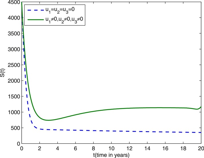
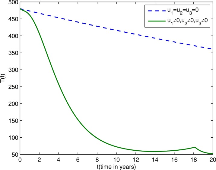
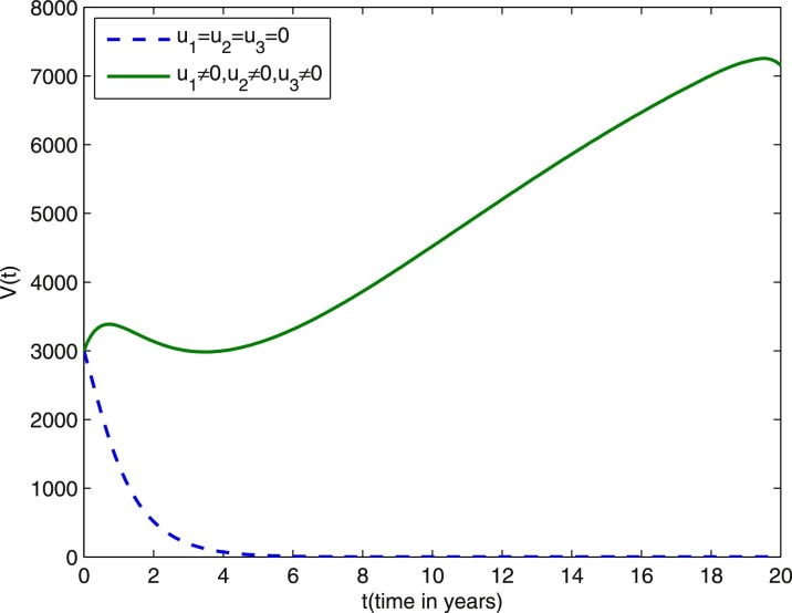
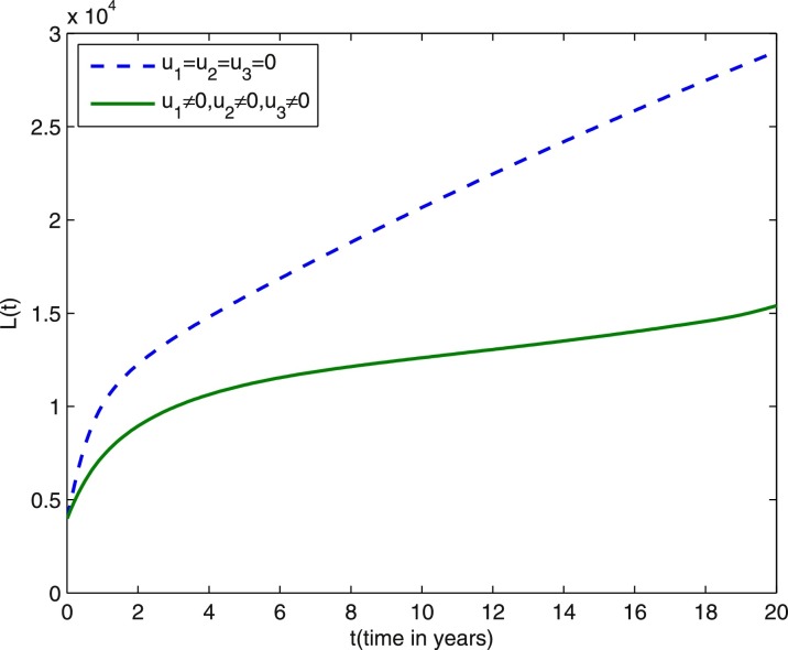
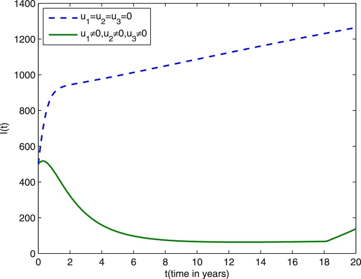
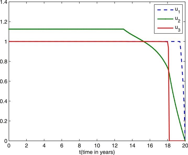
We start comparing the case of the population with optimal control actions and without control actions. In Figs. 1 –5, the population with optimal control actions are shown in solid lines, compared with the population without control actions which are shown in dashed lines. We observe from Fig. 1 that the susceptible population is higher under control compared to the case without control. The results in Fig. 2 predict a higher level of vaccinated population for the aforementioned tuberculosis intervention strategies under control compared to the case without control. The results depicted in Figs. 3 and 4 clearly suggest that the optimal control results are very effective in control of individuals infected with TB in latent stage and in the active stage, as expected. In Fig. 5, the population of treated humans declines sharply in the first 18 years and after that decrease further, while Fig. 4 shows slight increase in the last two years of the intervention strategy. This is due to the fact that the treatment control u ₃ becomes zero after 18 years. The simulation results in Fig. 6 suggest that this strategy would require that the vaccination control u ₁ should be at maximum for almost the entire period of intervention, while treatment controls u ₂ and u ₃ should maintain maximum efforts for 13 years and 18 years respectively before decreasing to zero.

Fig. 1.

Dashed line: susceptible population without optimal control. Solid line: susceptible population with optimal control. Weight constants are $B_1=20,B_2=100,B_3=200,B_4=100,B_5=8000,B_6=150,$ and other parameter values are presented in Table 1.

Fig. 5.

Dashed lines: treated population without optimal control. Solid lines: treated population with optimal control. Weight constants are $B_1=20,B_2=100,B_3=200,B_4=100,B_5=8000,B_6=150,$ and other parameter values are presented in Table 1.

Fig. 2.

Dashed line: vaccinated population without optimal control. Solid line: vaccinated population with optimal control. Weight constants are $B_1=20,B_2=100,B_3=200,B_4=100,B_5=8000,B_6=150,$ and other parameter values are presented in Table 1.

Fig. 3.

Dashed line: latent population without optimal control. Solid line: latent population with optimal control. Weight constants are $B_1=20,B_2=100,B_3=200,B_4=100,B_5=8000,B_6=150,$ and other parameter values are presented in Table 1.

Fig. 4.

Dashed line: infectious population without optimal control. Solid line: infectious population with optimal control. Weight constants are $B_1=20,B_2=100,B_3=200,B_4=100,B_5=8000,B_6=150,$ and other parameter values are presented in Table 1.

Fig. 6.

Three optimal control strategies profiles during 20 years. Weight constants are $B_1=20,B_2=100,B_3=200,B_4=100,B_5=8000,B_6=150,$ and other parameter values are presented in Table 1.

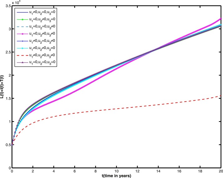
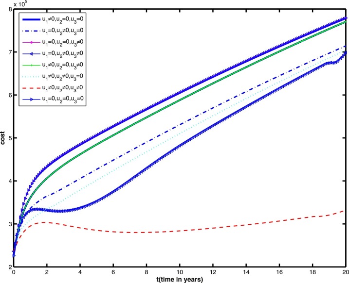
In what follows, we consider different control strategies in the reduction of infected individuals (including latent, infectious, being treated individuals). We observe in Fig. 7 that the infected individuals are lowest when three controls are considered. As the cost is one of the important parameter to decide for applicable strategy, we performed the cost design analysis and made comparative study of the cost for various strategies. The cost profiles for various control strategies are given in Fig. 8 . Note that the cost is least when three controls are considered, that is, the implementation of three control measures to restrict the epidemic while at the same time keeping the cost of vaccination and treatment very low are good policies for the achievement of our goal.

Fig. 7.

Infected individuals (including latent, infectious, being treated individuals) profiles under various control strategies during 20 years. Other parameter values are the same as those in Figs. 1–6.

Fig. 8.

Cost profiles under various control strategies during 20 years. Other parameter values are the same as those in Figs. 1–6.

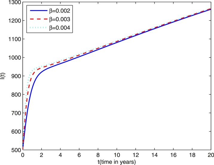
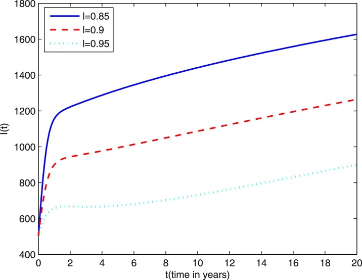
In Fig. 9 we present the effect of varying the disease transmission coefficient β on the number of individuals infected with TB in the active stage (I(t)). We observe that after about 12 years the effect of β is negligible on individuals infected with TB in the active stage. Fig. 10 shows the effect of varying fraction coefficient l on the number of individuals infected with TB in the active stage (I(t)). It is easy to see that the individuals infected with TB in the active stage affected much by l.

Fig. 9.

Simulations of TB model (1.2) showing the effect of varying transmission rates. Other parameter values are the same as those in Figs. 1–6.

Fig. 10.

Simulations of TB model (1.2) showing the effect of varying fraction coefficients. Other parameter values are the same as those in Figs. 1–6.

6. Conclusion

In this work, we have studied a simple mathematical model of TB presented by Liu and Zhang [24]. In order to control the spread of TB, we applied a preventive control in the form of vaccination and two treatment controls to susceptible, latent, and individuals infected with TB in the active stage. Next, we established the objective functional by remembering the fundamental biomedical goals in our mind. Theoretically, we proved the existence of optimal control and studied the characterization of optimal control by Pontryagin’s Maximum Principle. In order to assure that the optimal control is unique in the depictions, we investigated the uniqueness of the optimal control system.

Numerically, the simulations of the extended TB model (1.2) indicate that the vaccination and treatment strategies are effective in reducing TB disease transmission, especially we may get maximum disease control by using minimum cost as shown in Figs. 7 and 8. It could therefore be concluded that the comprehensive effect of all the three controls not only minimizes cost burden but also keeps a tab on infective population.

Undoubtedly, dynamics of TB infection is far more complicated and varied than the one captured by this mathematical model. Therefore, we will incorporate the time delay for drug resistance into the present model so as to provide us a better assessment for designing TB dynamics. In addition, we note that the principle technique for optimal control problem is to solve a set of “necessary conditions” that an optimal control and corresponding state must satisfy. If the Hamiltonian is linear in the control variable u, it would be difficult to solve for u* from the optimality equation. We will leave these cases as our future work.

References

- 1.World health organization, global tuberculosis control, 2012, http://www.who.int/en/, (accessed 2012).
- 2.World health organization, 2015, Tuberculosis Fact Sheet no.104. http://www.who.int/en/, (accessed March 2015).
- 3.Frieden T., Driver R.C. Tuberculosis control: past 10 years and future progress. Tuberculosis. 2003;83:82–85. doi: 10.1016/s1472-9792(02)00060-4. [DOI] [PubMed] [Google Scholar]
- 4.Raviglione M.C. Evolution of WHO, 1948–2001 policies for tuberculosis control. Lancet. 2002;359:775–780. doi: 10.1016/s0140-6736(02)07880-7. [DOI] [PubMed] [Google Scholar]
- 5.Raviglione M.C., Dye C., Schmizt S., Kochi A. For the global surveillance and monitoring project: assessment of worldwide tuberculosis control. Lancet. 1997;350:624–629. doi: 10.1016/s0140-6736(97)04146-9. [DOI] [PubMed] [Google Scholar]
- 6.Chiang C.Y., Riley L.W. Exogenous reinfection in tuberculosis. Lancet. Infect. Dis. 2005;5:629–636. doi: 10.1016/S1473-3099(05)70240-1. [DOI] [PubMed] [Google Scholar]
- 7.Feng Z., Castillo-Chavez C., Capurro A.F. A model for tuberculosis with exogenous reinfection. Theor. Popul. Biol. 2000;57:235–247. doi: 10.1006/tpbi.2000.1451. [DOI] [PubMed] [Google Scholar]
- 8.Jung E., Lenhart S., Feng Z. Optimal control of treatments in a two-strain tuberculosis model. Dis. Cont. Dyn. Syst. Ser. B. 2002;2(4):473–482. [Google Scholar]
- 9.Blayneh K., Cao Y., Kwon H.D. Optimal control of vector-borne diseases: treatment and prevention. Dis. Cont. Dyn. Syst. B. 2009;11(3):587–611. [Google Scholar]
- 10.Blower S.M., McLean A.R., Porco T.C., Small P.M., Hopewell P.C., Sanchez M.A., Moss A.R. The intrinsic transmission dynamics of tuberculosis epidemic. Nat. Med. 1995;1:815–821. doi: 10.1038/nm0895-815. [DOI] [PubMed] [Google Scholar]
- 11.Castillo-chavez C., Song B. Dynamical models of tuberculosis and their applications. Math. Biosci. Eng. 2004;1:361–404. doi: 10.3934/mbe.2004.1.361. [DOI] [PubMed] [Google Scholar]
- 12.Gaff H., Schaefer E. Optimal control applied to vaccination and treatment strategies for various epidemiological models. Math. Biosci. Eng. 2009;6:469–492. doi: 10.3934/mbe.2009.6.469. [DOI] [PubMed] [Google Scholar]
- 13.Khajanchi S., Ghosh D. The combined effects of optimal control in cancer remission. Appl. Math. Comput. 2015;271:375–388. [Google Scholar]
- 14.Kumar A., Srivastava P.K. Vaccination and treatment as control interventions in an infectious disease model with their cost optimization. Commun. Nonlinear Sci. Numer. Simul. 2017;44:334–343. [Google Scholar]
- 15.Lee J., Kim J., Kwon H.D. Optimal control of an influenza model with seasonal forcing and age-dependent transmission rates. J. Theor. Biol. 2013;317:310–320. doi: 10.1016/j.jtbi.2012.10.032. [DOI] [PubMed] [Google Scholar]
- 16.Zeiler I., Caulkins J.P., Grass D., Tragler G. Keeping options open:an optimal control model with trajectories that reach a DNSS point in positive time. SIAM J. Control. Optim. 2010;48(6):3698–3707. [Google Scholar]
- 17.Zhou Y.G., Liang Y.T., Wu J.H. An optimal strategy for HIV multitherapy. J. Comput. Appl. Math. 2014;263:326–337. [Google Scholar]
- 18.Blower S.M., Small P.M., Hopewell P.C. Control strategies for tuberculosis epidemics: new models for old problems. Science. 1996;273:497–500. doi: 10.1126/science.273.5274.497. [DOI] [PubMed] [Google Scholar]
- 19.Castillo-Chavez C., Feng Z. Mathematical models for the disease dynamics of tuberculosis. In: Horn M.A., Simonett G., Webb G., editors. Advances in Mathematical Population Dynamics-Molecules, Cells and Man. Vanderbilt University Press; Nashville: 1998. pp. 117–128. [Google Scholar]
- 20.Cohen T., Murray M. Modeling epidemics of multidrug-resistant m. tuberculosis of heterogeneous fitness. Nat. Med. 2004;10(10):1117–1121. doi: 10.1038/nm1110. [DOI] [PMC free article] [PubMed] [Google Scholar]
- 21.Dye C., Garnett G.P., Sleeman K., Williams B.G. Prospects for worldwide tuberculosis control under the who dots strategy. directly observed short-course therapy. Lancet. 1998;352(9144):1886–1891. doi: 10.1016/s0140-6736(98)03199-7. [DOI] [PubMed] [Google Scholar]
- 22.Gomes M., Franco A., Gomes M., Medley G. The reinfection threshold promotes variability in tuberculosis epidemiology and vaccine efficacy. Proc. R. Soc. B. 2004;271(1539):617–623. doi: 10.1098/rspb.2003.2606. [DOI] [PMC free article] [PubMed] [Google Scholar]
- 23.Vynnycky E., Fine P.E. The natural history of tuberculosis: the implications of age-dependent risks of disease and the role of reinfection. Epidemiol. Infect. 1997;119(2):183–201. doi: 10.1017/s0950268897007917. [DOI] [PMC free article] [PubMed] [Google Scholar]
- 24.Liu J.L., Zhang T.L. Global stability for a tuberculosis model. Math. Comput. Model. 2011;54:836–845. [Google Scholar]
- 25.Verver S., Warren R.M., Beyers N., Richardson M., van der Spuy G.D., Borgdorff M.W., Enarson D.A., Behr M.A., van Helden P.D. Rate of reinfection tuberculosis after successful treatment is higher than rate of new tuberculosis. Am. J. Respir. Crit. Care. Med. 2005;171:1430–1435. doi: 10.1164/rccm.200409-1200OC. [DOI] [PubMed] [Google Scholar]
- 26.Bowong S., Alaoui A.M.A. Optimal interventions strategies for tuberculosis. Commun. Nonlinear Sci. Numer. Simul. 2013;18:1441–1453. [Google Scholar]
- 27.Choi S., Jung E., Lee S.M. Optimal intervention strategy for prevention tuberculosis using a smoking-tuberculosis model. J. Theor. Biol. 2015;380:256–270. doi: 10.1016/j.jtbi.2015.05.022. [DOI] [PubMed] [Google Scholar]
- 28.Moualeu D.P., Weiser M., Ehrig R., Deuflhard P. Optimal control for a tuberculosis model with undected cases in cameroon. Commun. Nonlinear Sci. Numer. Simul. 2015;20:986–1003. [Google Scholar]
- 29.Mushayabasa S., Bhunu C.P. Modeling the impact of early therapy for latent tuberculosis patients and its optimal control analysis. J. Biol. Phys. 2013;39:723–747. doi: 10.1007/s10867-013-9328-6. [DOI] [PMC free article] [PubMed] [Google Scholar]
- 30.Rodrigues P., Silva C.J., Torres D.F.M. Cost-effectiveness analysis of optimal control measures for tuberculosis. Bull. Math. Biol. 2014;76(10):2627–2645. doi: 10.1007/s11538-014-0028-6. [DOI] [PubMed] [Google Scholar]
- 31.Silva C.J., Torres D.F.M. Optimal control applied to tuberculosis models. the IEA-EEF european congress of epidemiology 2012: epidemiology for a fair and healthy society. Eur. J. Epidemiol. 2012;27:S140–141. [Google Scholar]
- 32.Silva C.J., Torres D.F.M. Optimal control for a tuberculosis model with reinfection and post-exposure interventions. Math. Biosci. 2013;244(2):154–164. doi: 10.1016/j.mbs.2013.05.005. [DOI] [PubMed] [Google Scholar]
- 33.Silva C.J., Torres D.F.M. A TB-HIV/AIDS coinfection model and optimal control treatment. Dis. Cont. Dyn. Syst. A. 2015;35(9):4639–4663. [Google Scholar]
- 34.Yang Y.L., Tang S.Y., Ren X.H., Zhao H.W., Guo C.P. Global stability and optimal control for a tuberculosis model with vaccination and treatment. Dis. Cont. Dyn. Syst. Ser. B. 2016;21:1009–1022. [Google Scholar]
- 35.Fleming W.H., Rishel R.W. Springer-Verlag; New York: 1975. Deterministic and Stochastic Optimal Control. [Google Scholar]
- 36.Lenhart S.M., Workman J.T. CRC Press; 2007. Optimal Control Applied to Biological Models. [Google Scholar]
- 37.Pontryagin L.S. CRC Press; 1987. Mathematical Theory of Optimal Processes. [Google Scholar]