Abstract
Air pollutant transmission has significant influences on indoor air quality (IAQ). It is crucial to study mechanisms involved with airborne contaminant dispersion indoors. However, relationship between pollutant diffusion coefficient and viscosity in enclosed spaces has not been fully understood. In this study, turbulent Schmidt number (Sct) was modified as a function of turbulent kinematic viscosity rather than a constant value to better simulate dispersion of airborne contaminant in two typical enclosed spaces: an aircraft cabin and an office room. An experiment for airborne contaminant transmission was conducted in an aircraft cabin mockup. Combining with experimental data in the office room with an under floor air distribution (UFAD) system from literature, Sct was modified based on airflow vortex structures. The performance of RNG k-ε model using the modified Sct was found to be obviously better than that using the default Sct value in both the two enclosed spaces. In addition, model applicability to different enclosed spaces was analyzed based on the airflow vibration frequency.
Keywords: Vortex structure, Enclosed space, Turbulent Schmidt number, Contaminant dispersion, CFD
Highlights
-
•
Modified turbulent Schmidt number as a function of turbulent kinematic viscosity.
-
•
Conducted an experiment for the modification based on airflow vortex structure.
-
•
Analyzed the modification applicability to different enclosed spaces.
1. Introduction
Some confined vehicle cabins, such as aircraft cabins, provide an easy way for pathogens to spread. The virus laden bio-aerosols like severe acute respiratory syndrome (SARS) and H1N1-A influenza generated by infected occupants through coughing or sneezing can be transported throughout the cabin and infect other occupants, as reported by Wilder-Smith [1] and Baker et al. [2]. In residential buildings and other indoor environments, people are continuously exposed to different air pollutants. Aerosol particles are regarded as major pollutant sources, and they are closely related to such adverse health effects [3]. Other pollutants, such as formaldehyde and volatile organic chemicals (VOCs) can increase the risk of chronic toxicity and even cancer due to prolonged and high-dose exposure [4]. Therefore, it is important to study mechanisms involved in spreading of airborne contaminants, in order to prevent transmission and make a quick respond for chemical and biological attacks in enclosed environments as well.
For airborne contaminant transport, turbulent Schmidt number (Sc t) which represents the ratio between turbulent kinematic viscosity and turbulent diffusion coefficient is a key parameter for contaminant concentration prediction in turbulent airflow. Previous researchers have investigated the effect of Sc t on predicted contaminant dispersion for different situations. Sc t values ranged from 0.6 to 0.9 in computational fluid dynamics (CFD) simulations for urban diffusion problems [[5], [6], [7]]. For jet flow simulations, Sc t values were suggested to be 0.2 for jet-in-cross flow [8] and 0.9 for free round jet [9]. Riddle et al. [10] reported reducing the Sc t from its ‘‘standard value of 0.7″ to 0.3 could improve the predicted ground level concentrations. From these studies, Sc t varies in value for different local flow properties, indicating its value should be performed based on the airflow structures. Shi et al. [11] proposed a new dynamic turbulent Schmidt number model based on local velocity gradient and density gradient, while their study focused on Sc t in the boundary layer. Mokhtarzadeh-Dehghan et al. [12] found Sc t should be associated with Richardson number in order to model the experimental spreading rates of heavier-than-air gases correctly in an atmospheric boundary layer. However, they didn't consider local flow properties based on the airflow structures.
For the aircraft cabin and built environment, some researchers have investigated performances of different CFD models for airborne contaminant transport. Zhao et al. [13] and Zhang et al. [14] evaluated different Eulerian and Lagrangian models in enclosed spaces. Wang et al. [15] provided advanced turbulence models for predicting particle transport by integrating different numerical models. Zhao et al. [16] proposed an improved drift flux model to predict particle dispersion. However, these CFD models performed relatively poorly for concentration simulation. Some experimental studies were also conducted in aircraft cabins. Wang et al. [17] studied airborne contaminant transport using CO2 as a tracer gas inside an aircraft cabin. Sze To et al. [18] studied dispersion of expiratory droplets with mixing ventilation inside an aircraft cabin mockup. Zhang et al. [19] measured and predicted contaminant distributions in a cabin mockup. They used SF6 and mono-dispersed particles with diameter of 0.7 to simulate airborne contaminants. Li et al. [20] conducted an experiment for gaseous (SF6) and particulate (3 particle) contaminant dispersion in an actual functional MD-82 aircraft cabin. They stated that in narrow cabin space, source location and thermal buoyancy had a significant effect on airborne contaminant distributions. These research made a great contribution to understanding of contaminant transport in enclosed spaces, however, they did not analyze effect of different airflow structures on the Sc t value. Airflow in enclosed spaces is a kind of interaction of different flow structures, such as vorticity and deformation; therefore, the Sc t value should not be a constant number, but be varying based on airflow structures.
The objective of this study is to modify Sc t numbers to quantify the relationship between turbulent kinematic viscosity and turbulent diffusion coefficient. An experiment for airborne contaminant dispersion is conducted in a well-controlled aircraft cabin mockup. Combining with experimental data in an office room from literature, we establish new equations of the Sc t value based on different vortex structures in airflow. The improved models are then validated by laboratory experiments. In addition, through airflow frequency analysis, the reason for inconsistent equations of Sc t for different environments is explored.
2. Methodology
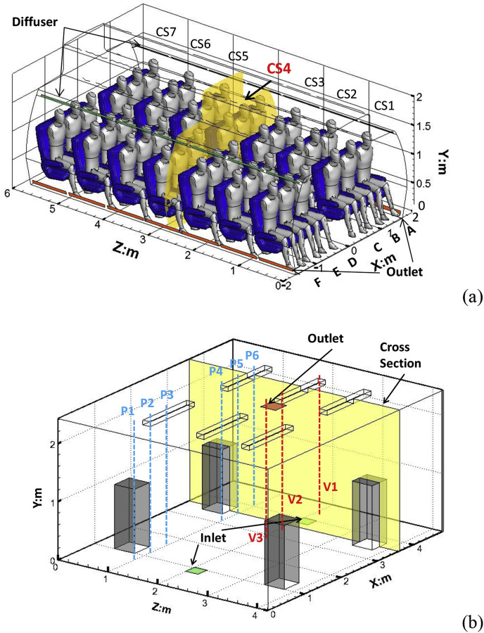
Two typical cases of enclosed space environment were selected for Sc t modification. As show in Fig. 1 (a), the first case is in the seven-row aircraft cabin mockup [21]. The cabin had 42 heated manikins with sensible heat production of 75 W for each. Air was supplied through two rows of diffusers on cabin shoulders and was exhausted at outlets located on side wall near the cabin floor, and the air change rate was 48 ACH. The second case is in the office with an under floor air distribution (UFAD) system [22] as shown in Fig. 1 (b). The room had four heated human simulators. Air was supplied from two floor inlets and exhausted from a ceiling outlet, and the air change rate was 5.5 ACH (air change per hour). Since modification of Sc t is associated with vortex structure, a numerical model was used to identify vortex structure firstly. .
Fig. 1.
Schematic of the seven-row aircraft cabin mockup (a) and office room (b).
2.1. Numerical procedure
In this study, three different turbulence models: RNG k-ε model, RSM model, and SST k- model were employed to calculate airflow distributions and compared with each other. The RNG k-ε model has been widely used for predicting indoor airflows with many successes [23]. The RSM turbulence model is more complex and more accurate with turbulent velocity fluctuations, but it needs more computing resource [24]. Martinho et al. [25] reported the SST model typically gave better results for heat transfer between the heating body and thermal environment. The governing equation of all these turbulence models equations can be written in a general form:
| (1) |
where is flow variables (velocity, enthalpy, turbulence parameters and mass fraction), is the effective diffusion coefficient, and is the source term. Details about coefficients and for different variables can be found in the Ansys theory guide [26].
Based on Eq. (1), the species transport equation can be written as:
| (2) |
where is local mass fraction, is turbulent kinematic viscosity, is the mass diffusion coefficient. Airflow distribution was solved by Eq. (1) first, then it was frozen, and the concentration field was simulated by Eq. (2). Default is 0.7 in most numerical simulations. However, as mentioned in the introduction part, should be determined by considering the flow structures [27]. The airflow field was simulated under steady state, and the gravity was considered. SIMPLE algorithm was applied to couple pressure and velocity, and standard and second-order were used for pressure discretization and all other variables. Residual was below 10−6 for energy and 10−3 for all other variables. Boussinesq approximation which is a common approach for indoor airflow simulations was employed to consider buoyancy effect. Standard wall treatment was applied to model near wall turbulence.
For the boundary conditions of the aircraft cabin, the inlet velocity direction was measured by ultrasonic anemometers (UAs), while the velocity magnitude was measured by hot-sphere anemometers (HSAs). Thermal boundaries of the walls and heating manikins were measured by an infrared camera. The measured data were assigned into the diffusers which had same effective areas as the real model through user-defined functions (UDFs). The pressure outlet boundary condition was applied on the exhausts, and the reference pressure value was set to 0 Pa. Tetra-mesh was used in this study, with total grid number of nine million, and the meshes closed to diffusers and manikins were refined. Details of boundary and mesh grid conditions for the office and aircraft cabin simulations can be found in Zhang et al. [22] and Li et al. [28] respectively.
In this study, the relationship between and was established based on vortex structure of airflow. Li et al. [21] used the Okubo-Weiss parameter, Q introduced by Okubo and Weiss to identify the type of vortex structure in an aircraft cabin. The parameter, Q is differential of deformation and vorticity square and its expression is:
| (3) |
where represents stretching deformation, represents shearing deformation, and represents vorticity as follows:
| (4) |
| (5) |
| (6) |
The interval of Q is always divided into three parts by 0.2 , where is standard deviation of in the entire fluid domain. When Q > 0.2 , the region is dominated by deformation; when Q < −0.2 , the region is dominated by vorticity; and when −0.2 < Q < 0.2, it is an ambient field. This standard was adopted to identify “deformation dominated region” and “vorticity dominated region” in the aircraft cabin and office room. and values in different regions were determined based on experimental data.
2.2. Validation of the numerical method
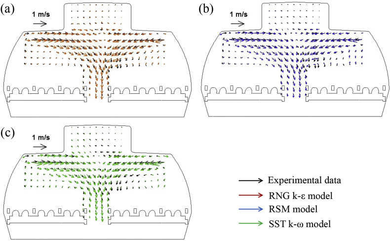
For the study on contaminant transport, airflow fields should be predicted correctly. Experimental data from literature was used to validate the numerical model. Fig. 2 shows comparison of experimental data from particle image velocimetry (PIV) measurement [29] with simulated airflow patterns in CS4 of the aircraft cabin (Fig. 1 (a)) by three turbulence models. As shown in Fig. 2, decay of the simulated velocity is slower than the experiment due to underestimated turbulence kinetic energy [30]. The predicted airflow fields from all turbulence models were similar and all captured the trend of PIV measured airflow. Jets from right and left diffusers merged in the middle, and the jet from the left side was a little stronger due to the asymmetry diffuser conditions in the cabin. In addition, velocity magnitudes were lower in top and side regions.
Fig. 2.
Comparison of the simulated airflow patterns with the experimental data from Li et al. [29].
However, remarkable differences exist if we look at the two sets of vectors at certain positions, especially in the middle where the jets from right and left merged. The inlet velocity direction was measured by UAs, whose probes could not be placed very close to the diffusers [31]. This maybe resulted in some errors of measured velocity direction. The experimental data may unavoidably have some instrumental errors and thereby lead to some deviations in the center of the cabin where the velocity was very small (<0.1 m/s).
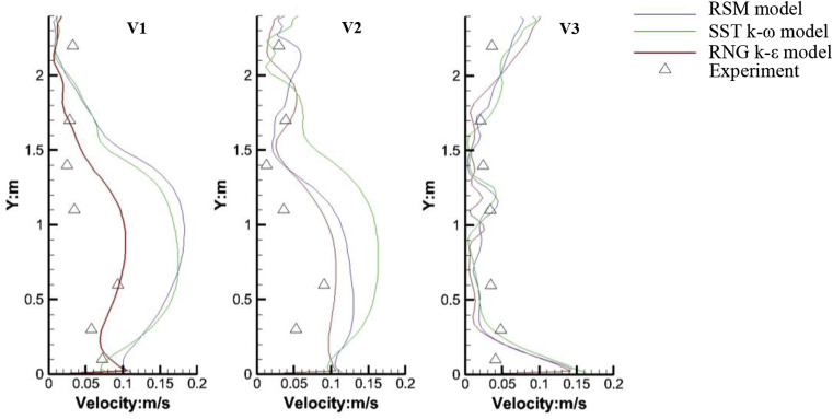
Fig. 3 shows comparison of predicted airflow velocities with experimental data [22] at poles V1 to V3 for the office room (Fig. 1 (b)) by different turbulence models. Poles V1 to V3 were in the vicinity of the selected cross section. From Fig. 3, the simulated data by RNG k-ε model agrees best with the measured data. While the RSM model performs worst, which may be caused by its convergence problem in three-dimensional buoyant flow [23]. The simulation agreed better with measured data at lower and top part of pole V1 and V2, but worse in the middle part of pole V1 and V2. For pole V3, predicted and experimental velocities were all lower in the middle part, but discrepancies were significant at its top and lower parts.
Fig. 3.
Comparison of the predicted airflow velocities with the experimental data from Zhang et al. [22].
RRMSE (relative root mean square error) was used to conduct quantitative comparison between different turbulence models:
| (7) |
where are experimental and simulated concentration at sampling point i. is average experimental concentration. Table 1 shows the RRMSE values for three turbulence models. For the aircraft cabin, the RNG k-ε model performs slightly better. Considering overall low velocities and complex turbulent flow in the cabin, the difference between these turbulence models is not observable. For the office room, performance of the RNG k-ε model is much better than other models. Overall, the RNG k-ε model performed the best in both spaces, and its predicted airflow fields were also acceptable. Taking the computing efforts into consideration, it was employed to modify the turbulent Schmidt number in this study.
Table 1.
RRMSE for evaluating velocity predicted by three turbulence models.
| RNG k-ε | RSM | SST k- | |
|---|---|---|---|
| Aircraft cabin | 0.38 | 0.44 | 0.39 |
| Office room | 0.46 | 0.70 | 0.53 |
2.3. Turbulent Schmidt number modification
Goldman et al. [32] investigated values for different working gases in an air pipe. In the pipe under steady condition, the concentration distribution can be expressed as Eq. (3) as follows:
| (8) |
where C and is concentration and average axial fluid velocity. M is source strength, and is the effective diffusion coefficient. With a known M, through measuring concentration (C), velocity () and coordinate (X, r) in the pipe, an effective diffusion coefficient () can be calculated through Eq. (8). in the pipe can be also calculated by empirical formulas [33]. Accordingly, corresponding to one value, one value can be obtained. Goldman et al. [32] used this method to study the relationship between and in the air pipe. They developed a fitting equation to express their relationship:
| (9) |
where and are laminar kinematic viscosity and laminar Schmidt number. They are dependent on air and released working gas property.
In enclosed space environment, the situation was much more complicated than that in the air pipe. cannot be calculated through analytic equations like Eq. (8), and no empirical formula can be used to calculate the value as well. However, CFD provided a useful tool to solve this problem. In the RNG k-ε model, values can be calculated as follow:
| (10) |
where is a constant number, is turbulence kinetic energy, and is turbulence dissipation. Through repeated numerical trial calculation, values in different regions can also be obtained. Referring to Eq. (9), relationship between and can be expressed as a unified equation for a certain working gas:
| (11) |
where b and c are undetermined parameters. In the laminar layer, approaches zero, should approach unity, and mass diffusion coefficient controls the dispersion. In the turbulent core region, is high, approaches unity as well, and turbulent diffusion coefficient governs the dispersion. Unlike Goldman's study, only one pair of working gases (air - SF6) was used in our study, and b and c were constant. Therefore, it needed two sets of and data to determine these two parameters.
2.3.1. Source setting
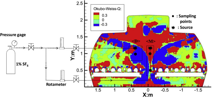
Fig. 4 shows the predicted Q value in section CS4 of the aircraft cabin (Fig. 1 (a)). Blue regions are dominated by vorticity, red regions in the figure are dominated by deformation, and green regions are ambient fields. The Q value was higher in the vicinity of diffusers and at the aisle where two air jets from diffusers merged. While, the Q value was lower in the sides of the cabin due to two large flow re-circulations on each side. Two regions <D> and <M> with different vortex structures (Fig. 4) were selected to reveal the relationship between and in the aircraft cabin. In region <M>, source M was elected in the middle of the aisle dominated by deformation. Contaminant released from source M was transported downward by airflow and directly exhausted from the cabin. In region <D>, source D was at the breathing level of a passenger dominated by vorticity. Contaminant released from source D could travels repeatedly in region <D> and was locked up by eddy airflow. Mixed tracer gas (1% sulfur hexafluoride-SF6, 99% N2 balance) was released from a rubber bulb recommended by Li et al. [20]. Diameter of the rubber bulb was 5 cm, and 200 holes with diameter of 2 mm were distributed on the bulb surface to make an almost zero momentum release. Volume flow rate of the mixed tracer gas released from each source was set to 1 L/min and was controlled through two gas rotameters with relative errors of 4% (Fig. 4).
Fig. 4.
Schematic of the experiment system and predicted vortex structure in section CS4 of the aircraft cabin.
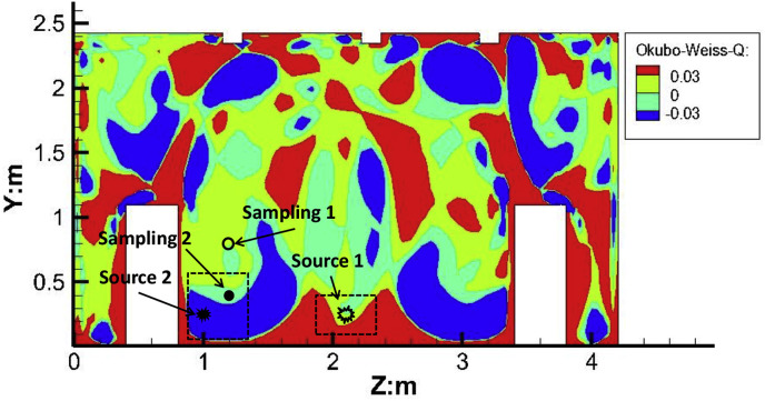
Fig. 5 shows the predicted Q value in the cross section of the office room (Fig. 1 (b)). The Q value was higher near the middle of the floor, and lower in the vicinity of manikins. Two regions with different vortex structures (Fig. 5) were selected. Source 2 was in the vorticity dominated region of the cross section (X = 3.6 m), and Source 1 was in the deformation dominated region of the cross section (X = 3.28). Particles with mean diameter of 0.7 were used in their study. Murakami [34] and Li et al. [20] reported particles smaller than 3 have the similar concentration distribution as tracer gas in the room and aircraft cabin respectively. Therefore, concentration distributions for 0.7 particles could be used as a surrogate for that of SF6.
Fig. 5.
Predicted vortex structure in the cross section of the office room with an UFAD system.
2.3.2. Sampling setting
Concentration distributions with each source working in the aircraft cabin were analyzed with a photo-acoustic multi-gas analyzer (INNOVA 1412, LumaSense Technologies) whose lower detection limit is 0.06 ppm for SF6. Twelve sampling points including sampling points in region <D> and <M> were employed to cover CS3, CS4, and CS5 (Fig. 1 (a)), totally 36 sampling points. Sampling time of each point was set to be 3τ (τ is the time constant which is the volume of the cabin divided by the ventilation rate, and it is 80 s in this study). This is because, under the hypotheses of well mixed, air in a cabin can be exchanged fully after 3τ [35], and concentration volatility and uncertainty can be captured in this period. Accordingly, for each sampling point, measured data in 240 s were used to determine its averaged concentration and confidence interval.
For the office room, a particle counter (PC-2H QCM impactor, California Measurements Inc.) was used to measure particle concentration in six locations (poles P1 to P6) as shown in Fig. 1 (b) at five different heights, totally 30 sampling points. Sampling 2 in the vorticity dominated region of the cross section (X = 3.6 m) was elected to be paired with Source 2 (Fig. 5). In Zhang's study [22], no sampling point was set in the deformation dominated region of the cross section (X = 3.28) closed to Source 1; therefore, Sampling 1 on streamlines from the region was elected to match with Source 1.
3. Results
3.1. Improved model solution
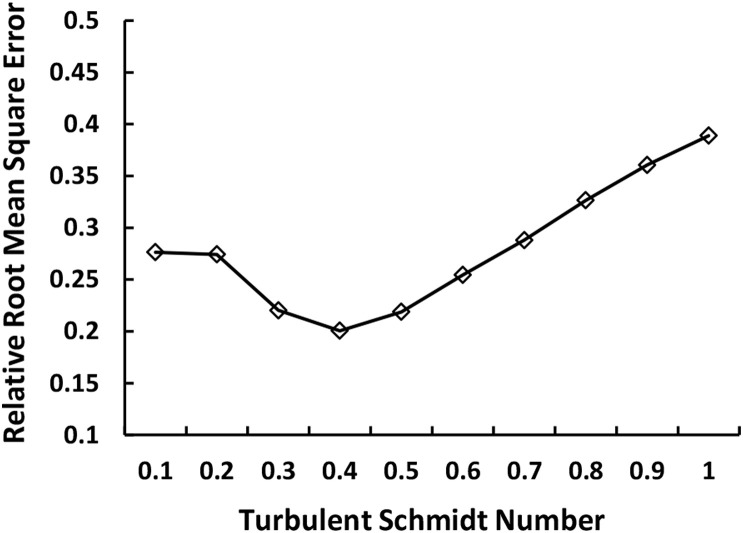
For the aircraft cabin, the averaged value was about 0.00040 m2/s in region <D>, and 0.00073 m2/s in region <M>. Through adjusting in numerical simulation and comparing predicted data with experimental data in the region, in each region was got by repeated trial calculations. Taking region <M> for example, the repeated trial calculation started from = 0.7, and the value with the smallest relative root mean square error (RRMSE, Eq. (13)) between predicted and experimental data in region <M> was 0.4, as illustrated in Fig. 6 . Similarly, the value for the region <D> was 0.05.
Fig. 6.
Relative root mean square errors for region <M> in the aircraft cabin with different Sct values.
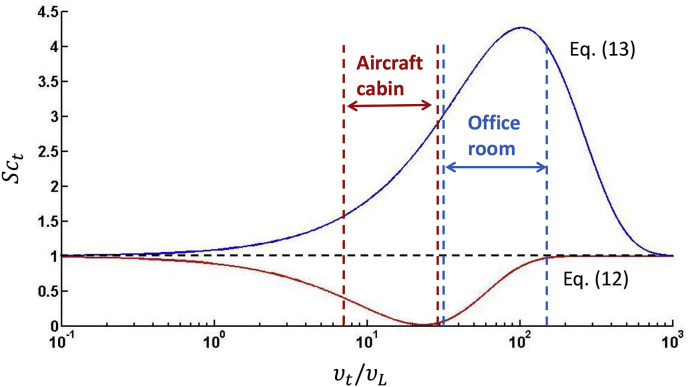
By inputting and of these two regions <D> and <M> into Eq. (7), b is 0.12, and c is 0.043. Therefore, the relationship between and in the aircraft cabin can be expressed as:
| (12) |
For the office room, through the similar method, averaging values in the two regions were calculated by Eq. (10) based on the RNG k-ε model; and the value in each region was got by repeated trial calculation as well. The relationship between and in the office room can be expressed as:
| (13) |
Implementing Eq. (12) and Eq. (13) through user defined functions (UDFs), the numerical model could be used to simulate contaminant distributions in the cabin mockup and office room.
3.2. Comparison of the improved models with the existing solution
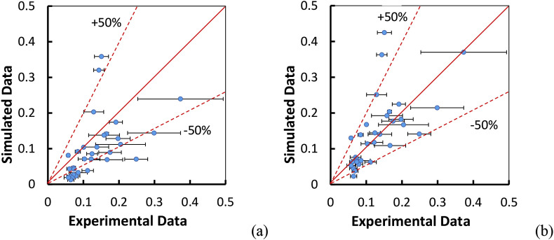
To test effectiveness of the improved Sc t model in different enclosed spaces, comparison of improved model with existing solution (Sc t = 0.7) was conducted. It should be noted that the data employed to develop the model were not used to validate the model. For the aircraft cabin, the data in the region <D> and <M> (Fig. 4) were used to improve the model, while all the data in CS3, CS4 and CS5 were used to validate the model. For the office room, the data in the two regions were used to develop the model, while all the data in poles P1-P5 were used to validate the model. Normalized concentrations for Source D from the simulation and experiment in CS3, CS4 and CS5 were plotted against each other in Fig. 7 . The solid line represents perfect agreement, the dotted lines represent the region with errors ranging from −50% to 50%, and the error bars presented 95% confidence intervals. RRMSE and another index, correlation coefficient (r) were employed to quantify concentration data comparison. The correlation coefficient (r) [36] is defined as follows:
| (14) |
where are experimental and simulated concentration at sampling point i. are averaging concentration of experiment and simulation. The correlation coefficient (r) describes the linear correlation of the experimental and predicted data. It ranges from −1 to 1, with −1 meaning strong negative relationship, 0 meaning no relationship and 1 meaning strong positive relationship. As shown in Fig. 7 and Table 2 , for the aircraft cabin, the simulated result using the modified Sc t model was obviously better than that using the default Sc t, and it has a lower relative root mean square error and higher correlation coefficient.
Fig. 7.
Comparison of the experimental data with predicted SF6 concentrations by: (a) default Sct (0.7), (b) modified Sct (Eq. (12)) in the aircraft cabin.
Table 2.
RRMSE and r with default and modified Sct.
| Solution | RRSME | ||
|---|---|---|---|
| Aircraft cabin | Model with default Sct | 1.13 | 0.32 |
| Model with modified Sct | 0.82 | 0.65 | |
| Office room | Model with default Sct | 1.20 | 0.74 |
| Model with modified Sct | 0.92 | 0.73 |
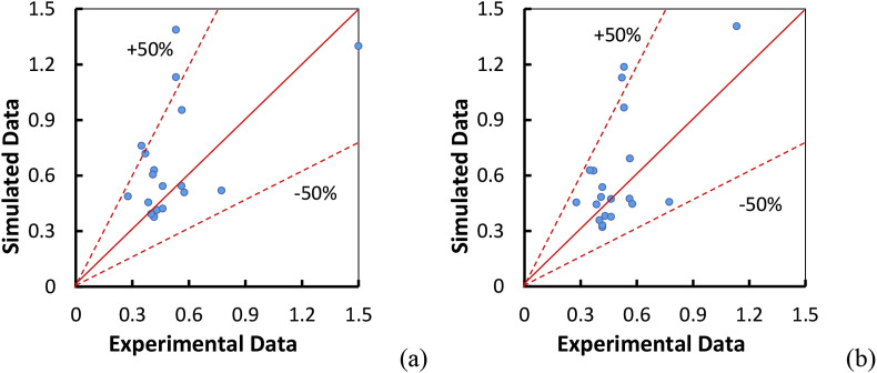
For the office room with an UFAD system, normalized concentrations from the simulation and experiment in poles P1-P5 were also plotted against each other in Fig. 8 . As shown in Fig. 8, more points from the improved Sc t model fall in the region with errors ranging from −50% to 50% and are closed to the solid line represents perfect agreement. This also can be confirmed in Table 2, in which RRSME is reduced from 1.20 to 0.92. However, the correlation coefficient does not have improvement; and it is almost identical for default Sc t and modified Sc t. This may be due to the fact that the correlation coefficient was already high relatively, and it was difficult to be improved further.
Fig. 8.
Comparison of the experimental data with simulated concentrations by: (a) default Sct (0.7), (b) modified Sct (Eq. (12)) in the office room.
4. Discussion
In this study, relationship between Sc t and for different vortex structures was revealed. When comparing Table 1 with Table 2, it is found that the RRMSE of predicted velocity is smaller than that of concentration. This is because the species transport equation is solved based on momentum equations, and a little discrepancy for the simulated velocity fields will lead to large discrepancy for the predicted concentration distributions. Therefore, discrepancy for the simulated velocity fields may result in lack of improvement of the proposed procedure. Additionally, because pipe flow and air cabin flow significantly differed, application of the equation deduced from pipe flow may also result in some limited improvement. However the modified Sc t model was still better than that using the default Sc t, because the modified Sc t can compensate underestimation of turbulent diffusion in the RNG k-ε model to some extent.
For other turbulence models, because predicted may be different with that from the RNG k-ε model, the Sc t expression function may have different parameters and need further investigation. Bazdidi-Tehrani et al. [37] proposed various non-linear eddy viscosity turbulence models and reported the traditional k-ε model using the Boussinesq's isotropic linear eddy-viscosity concept could overproduce turbulence kinetic energy at impingement zone and failed to predict complex flow structures around buildings. However, their study focused on flow and concentration fields on and around an isolated cubical building within the neutral turbulent boundary layer. Different with the turbulent core region in enclosed spaces, it is well known that, in the boundary layer, the turbulence is assumed to be anisotropic. In addition, some turbulence models, such as the v2-f model [38], were also proposed to predict anisotropic turbulence near the wall and solve overestimated turbulence fluctuation perpendicular to the wall.
Fig. 9 illustrated the modified Sc t equations and ranges of values for the selected different vortex structures in the aircraft cabin and office room. In these two spaces, most of the values fall within these ranges, but are not limited to these ranges. Because the equations of the modified Sc t are nonnegative and have specific physical meaning mentioned above, their effective ranges can cover all of the values in these two spaces. As shown in Fig. 9, equations of the modified Sc t are observably different for the aircraft cabin (Eq. (12)) and office room (Eq. (13)). We thought this may be caused by different airflow vibration frequencies. According to Prandtl's theory, vibration frequency is , where is mean fluctuation velocity, and l, per Shu's suggestion [39], should be the Kolmogorov scale as follows:
| (15) |
where is kinetic viscosity, is turbulence eddy dissipation. As it is well expected that and is the highest at air inlet, where the vibration frequency should be also highest there, we use at the inlet boundary to calculate vibration frequency. The inlet dissipation can be estimated as [26]:
| (16) |
| (17) |
where is mean velocity, k is turbulence kinetic energy, I is turbulence intensity, is the turbulence length scale (m), equals to 0.07 d, d is the hydraulic diameter of the inlet plane and . For the aircraft cabin, mean velocity of its inlets is 1.87 m/s [28], and turbulence intensity is 40% [40]. For the room, mean velocity of its inlets is 0.76 m/s, and turbulence intensity is 10–15% [22]. Accordingly, vibration frequency of airflow in the aircraft cabin is 12678 Hz, while it is 92 Hz in the office room with an UFAD system. The remarkable difference of airflow frequency between the aircraft cabin and office room may lead to different modified Sc t expression functions. Higher frequency may result in stronger diffusion ability corresponding to a lower Sc t value, and the relationship between airflow vibration frequency and Schmidt number need further research. Nevertheless, the proposed modification method expressing Sc t values as a function of associated with vortex structures can improve contaminant concentration prediction in turbulent flow. For other researchers in the field, if the enclosed spaces which they investigated have similar airflow structures and frequencies with ours, they can refer to our new Schmidt number; otherwise they can still use our method to modify the turbulent Schmidt number for their research.
Fig. 9.
Turbulent Schmidt numbers for different enclosed spaces.
5. Conclusions
In this paper, a method to modify Sc t as a function of turbulent kinematic viscosity based on airflow vortex structures was introduced to better simulate dispersion of airborne contaminant in two typical enclosed spaces: an aircraft cabin and an office room. This study was focused on gaseous pollutants, which are common in indoor environments. Three turbulence models were evaluated. The RNG k-ε model performed the best and was employed to modify Sc t. During the modification, different airflow vortex structures including deformation and vorticity were taken into consideration. Comparing with the experimental data, performance of the RNG k-ε model using modified Sc t was found to be better than that using default Sc t value in both the two enclosed spaces. For the aircraft cabin environment, the improved model reduced the relative root mean square error from 1.13 to 0.82, and increased the correlation coefficient from 0.32 to 0.65. For the office room with an UFAD system, the improved model reduced the relative root mean square error from 1.20 to 0.92, but no observable increase was found in correlation coefficient. The application of proposed modified method for different turbulence models and environments with different airflow vibration frequencies needs further research.
Acknowledgement
The research presented in this paper was supported financially by the National Science Foundation of China (NSFC) through Grant No. 51478301 and No. 51708286.
Nomenclature
- Sct
Turbulent Schmidt number
Laminar Schmidt number
Concentration
Mass diffusion coefficient (m2/s)
Fluid velocity (m/s)
Mean velocity (m/s)
- I
Turbulence intensity
- Q
Differential of deformation and vorticity square
- M
Source strength
- S
Source term
Mean fluctuation velocity (m/s)
- l
Kolmogorov scale (m)
Turbulence length scale (m)
- d
Hydraulic diameter (m)
- UFAD
Under Floor Air Distribution
- ACH
Air Change per Hour
- RANS
Reynolds-Averaged Navier-Stokes
- RNG
Renormalization Group
- HSA
Hot-Sphere Anemometers
- UAs
Ultrasonic Anemometers
- UDFs
User Defined Functions
- GCI
Grid Convergence Index
- RRMSE
Relative Root Mean Square Error
- PIV
Particle Image Velocimetry
Greek symbols
Flow variables
Effective diffusion coefficient (m2/s)
Turbulent kinematic viscosity (m2/s)
Laminar kinematic viscosity (m2/s)
Turbulence dissipation (m2/s3)
- τ
Time constant (s)
Turbulence kinetic energy (m2/s2)
- r
Correlation coefficient
References
- 1.Wilder-Smith A. The severe acute respiratory syndrome: impact on travel and tourism. Trav. Med. Infect. Dis. 2006;4(2):53–60. doi: 10.1016/j.tmaid.2005.04.004. [DOI] [PMC free article] [PubMed] [Google Scholar]
- 2.Baker M.G., Thornley C.N., Mills C., Roberts S., Perera S., Peters J., Kelso A., Barr I., Wilson N. Transmission of pandemic A/H1N1 2009 influenza on passenger aircraft: retrospective cohort study. Bmj. 2010;340 doi: 10.1136/bmj.c2424. [DOI] [PMC free article] [PubMed] [Google Scholar]
- 3.Bachmann J.D., Damberg R.J., Caldwell J.C. Environmental Protection Agency; Research Triangle Park, NC (United States): 1996. Review of the National Ambient Air Quality Standards for Particulate Matter: policy Assessment of Scientific and Technical Information. [Google Scholar]
- 4.Formaldehyde, 2-butoxyethanol and 1-tert-butoxypropan-2-ol, IARC Monographs on the Evaluation of Carcinogenic Risks to Humans. World Health Organization International Agency for Research on Cancer; , Lyon, France: 2006. [PMC free article] [PubMed] [Google Scholar]
- 5.Brzoska M.A., Stock D., Lamb B. Determination of plume capture by the building wake. J. Wind Eng. Ind. Aerod. 1997;67:909–922. [Google Scholar]
- 6.Lien F., Yee E., Ji H., Keats A., Hsieh K. Progress and challenges in the development of physically-based numerical models for prediction of flow and contaminant dispersion in the urban environment. Int. J. Comput. Fluid Dynam. 2006;20(5):323–337. [Google Scholar]
- 7.Santiago J.L., Martilli A., Martín F. CFD simulation of airflow over a regular array of cubes. Part I: three-dimensional simulation of the flow and validation with wind-tunnel measurements. Boundary-Layer Meteorol. 2007;122(3):609–634. [Google Scholar]
- 8.He G., Guo Y., Hsu A.T. The effect of Schmidt number on turbulent scalar mixing in a jet-in-crossflow. Int. J. Heat Mass Tran. 1999;42(20):3727–3738. [Google Scholar]
- 9.Yimer I., Campbell I., Jiang L.-Y. Estimation of the turbulent Schmidt number from experimental profiles of axial velocity and concentration for high-Reynolds-number jet flows. Can. Aeronaut. Space J. 2002;48(3):195–200. [Google Scholar]
- 10.Riddle A., Carruthers D., Sharpe A., McHugh C., Stocker J. Comparisons between FLUENT and ADMS for atmospheric dispersion modelling. Atmos. Environ. 2004;38(7):1029–1038. [Google Scholar]
- 11.Shi Z., Chen J., Chen Q. On the turbulence models and turbulent Schmidt number in simulating stratified flows. J. Build. Perform. Simul. 2015:1–15. [Google Scholar]
- 12.Mokhtarzadeh-Dehghan M., Akcayoglu A., Robins A. Numerical study and comparison with experiment of dispersion of a heavier-than-air gas in a simulated neutral atmospheric boundary layer. J. Wind Eng. Ind. Aerod. 2012;110:10–24. [Google Scholar]
- 13.Zhao B., Yang C., Yang X., Liu S. Particle dispersion and deposition in ventilated rooms: testing and evaluation of different Eulerian and Lagrangian models. Build. Environ. 2008;43(4):388–397. [Google Scholar]
- 14.Zhang Z., Chen Q. Comparison of the Eulerian and Lagrangian methods for predicting particle transport in enclosed spaces. Atmos. Environ. 2007;41(25):5236–5248. [Google Scholar]
- 15.Wang M., Lin C.-H., Chen Q. Advanced turbulence models for predicting particle transport in enclosed environments. Build. Environ. 2012;47:40–49. [Google Scholar]
- 16.Zhao B., Chen C., Tan Z. Modeling of ultrafine particle dispersion in indoor environments with an improved drift flux model. J. Aerosol Sci. 2009;40(1):29–43. [Google Scholar]
- 17.Wang A., Zhang Y., Topmiller J.L., Bennett J.S., Dunn K.H. Tracer study of airborne disease transmission in an aircraft cabin mock-up. ASHRAE Trans. 2006:697–705. [Google Scholar]
- 18.Sze To G., Wan M., Chao C., Fang L., Melikov A. Experimental study of dispersion and deposition of expiratory aerosols in aircraft cabins and impact on infectious disease transmission. Aerosol. Sci. Technol. 2009;43(5):466–485. [Google Scholar]
- 19.Zhang Z., Chen X., Mazumdar S., Zhang T., Chen Q. Experimental and numerical investigation of airflow and contaminant transport in an airliner cabin mockup. Build. Environ. 2009;44(1):85–94. [Google Scholar]
- 20.Li F., Liu J., Pei J., Lin C.-H., Chen Q. Experimental study of gaseous and particulate contaminants distribution in an aircraft cabin. Atmos. Environ. 2014;85:223–233. doi: 10.1016/j.atmosenv.2013.11.049. [DOI] [PMC free article] [PubMed] [Google Scholar]
- 21.Li F., Liu J., Ren J., Cao X., Zhu Y. Numerical investigation of airborne contaminant transport under different vortex structures in the aircraft cabin. Int. J. Heat Mass Tran. 2016;96:287–295. doi: 10.1016/j.ijheatmasstransfer.2016.01.004. [DOI] [PMC free article] [PubMed] [Google Scholar]
- 22.Zhang Z., Chen Q. Experimental measurements and numerical simulations of particle transport and distribution in ventilated rooms. Atmos. Environ. 2006;40(18):3396–3408. [Google Scholar]
- 23.Zhang Z., Zhang W., Zhai Z., Chen Q. Evaluation of various turbulence models in predicting airflow and turbulence in enclosed environments by CFD: Part 2—comparison with experimental data from literature. HVAC R Res. 2007;13(6):871–886. [Google Scholar]
- 24.Chen Q. Prediction of room air motion by Reynolds-stress models. Build. Environ. 1996;31(3):233–244. [Google Scholar]
- 25.Martinho N., Lopes A., da Silva M.G. Evaluation of errors on the CFD computation of air flow and heat transfer around the human body. Build. Environ. 2012;58:58–69. [Google Scholar]
- 26.Ansys A.F. ANSYS inc; 2011. 14.0 Theory Guide. [Google Scholar]
- 27.Tominaga Y., Stathopoulos T. Turbulent Schmidt numbers for CFD analysis with various types of flowfield. Atmos. Environ. 2007;41(37):8091–8099. [Google Scholar]
- 28.Li M., Zhao B., Tu J., Yan Y. Study on the carbon dioxide lockup phenomenon in aircraft cabin by computational fluid dynamics. Build. Simul. 2015:1–11. [Google Scholar]
- 29.Li J., Cao X., Liu J., Wang C., Zhang Y. Global airflow field distribution in a cabin mock-up measured via large-scale 2D-PIV. Build. Environ. 2015;(93):234–244. [Google Scholar]
- 30.Lin C., Dunn K., Horstman R., Topmiller J., Ahlers M., Bennett J., Sedgwick L., Wirogo S. Numerical simulation of airflow and airborne pathogen transport in aircraft Cabins–Part I: numerical simulation of the flow field. ASHRAE Trans. 2005;111(1) [Google Scholar]
- 31.Liu W., Wen J., Lin C.-H., Liu J., Long Z., Chen Q. Evaluation of various categories of turbulence models for predicting air distribution in an airliner cabin. Build. Environ. 2013;65:118–131. [Google Scholar]
- 32.Goldman I., Marchello J. Turbulent schmidt numbers. Int. J. Heat Mass Tran. 1969;12(7):797–802. [Google Scholar]
- 33.Deissler R.G. Turbulent heat transfer and friction in the entrance regions of smooth passages. Trans. ASME. 1955;77(8):1221–1232. [Google Scholar]
- 34.Murakami S. Diffusion characteristics of airborne particles with gravitational setting in an convection-dominant indoor flow field. ASHRAE Trans. 1992;98(1):82–97. [Google Scholar]
- 35.Etheridge D., Sandberg M. John Wiley & Sons; Chichester, USA: 1996. Building Ventilation: theory and Measurement. [Google Scholar]
- 36.Rice J. Nelson Education; 2006. Mathematical Statistics and Data Analysis. [Google Scholar]
- 37.Bazdidi-Tehrani F., Mohammadi-Ahmar A., Kiamansouri M., Jadidi M. Investigation of various non-linear eddy viscosity turbulence models for simulating flow and pollutant dispersion on and around a cubical model building. Build. Simul. 2015;(8):149–166. [Google Scholar]
- 38.Davidson L., Nielsen P.V., Sveningsson A. Proceedings of the International Symposium on Turbulence. 2003. Modifications of the ú2-model for computing the flow. [Google Scholar]
- 39.Shu W. The tracking behavior of scattered particles in turbulence. J. Tianjin Univ. 1970;(1):75–83. [Google Scholar]
- 40.Wei W., Nan J., Xiaodong C., Chen S., Junjie L. HWA measurement and analysis of MD-82 aircraft cabin environment flow field (in Chinese) J. Tianjin Univ. 2013;46(1):1–6sss. [Google Scholar]


