True epidemic growth construction through harmonic analysis

Highlights

• •A new way of regrouping epidemic reported data.
• •Construction of wavelets for the unadjusted and adjusted reported data.
• •Practically implementable method to construct true epidemic in an emerging epidemic.

Abstract

In this paper, we have proposed a two-phase procedure (combining discrete graphs and wavelets) for constructing true epidemic growth. In the first phase, a graph-theory-based approach was developed to update partial data available and in the second phase, we used this partial data to generate plausible complete data through wavelets. We have provided two numerical examples. This procedure is novel and implementable and adaptable to machine learning modeling framework.

1. Basis, motivation and introduction

In general, it is not easy to build a true epidemic growth curve in a timely fashion for any newly emerging epidemic, and the chances of building a true growth picture worsen with poor disease reporting. As we know, preparedness for the epidemic spread is a primary public health concern for any health department. Epidemic reporting of a disease is a fundamental event in understanding two key parameters in epidemiology, namely, epidemic diffusion within a population and growth at a population level. Normally, for a real-time epidemic, the reporting of cases is rarely complete, especially if the epidemic is new or symptoms are unknown or are yet to be discovered. For viruses with shorter incubation periods without virus shedding during the incubation period, any delay in reporting or lack of reporting could lead to a severe epidemic due to the absence of control measures. For example, for the Ebola virus, the average incubation period is between 2 and 21 days, and an individual diagnosed with the Ebola virus does not spread the virus to others during this period. If some of these individuals with Ebola are not diagnosed (and hence not reported to health care facilities) then after 21 days, these individuals will (unknowingly) spread the virus to others. There are other viruses whose incubation period is short but they are contagious during this period, for example, influenza. Even for epidemics with established symptoms, reporting could be nowhere close to complete. The impact of reporting on epidemic surveillance can then be theoretically measured (Rao, 2012).

Wavelet theory was developed fairly recently (about 35–40 years ago), but applications of wave functions fitted to epidemic data were seen more than 60 years ago (for example, Soper, 1929, Bartlett, 1956, and Bartlett, 1957). The observations by Bartlett (1957) on population size and the fraction of measles infecting people over various time points provided a new basis for using stochastic models for understanding retrospectively the seasonality of epidemics. This study by Bartlett (1957) and other studies (for example, see the summary in the book by Anderson and May, 1991) consider wave-like fitting of a time series data of epidemics. Bartlett, in his articles Bartlett, 1956, Bartlett, 1957 considered two differential equations to investigate small oscillations around the equilibrium. Earlier than this, a stochastic formulation of such models was seen by Soper in his paper Soper (1929).

Suppose i(t) and s(t) represent infected and susceptible numbers at time t. A simple ODE considered by Bartlett (which was improvisation of the model by Soper (1929)) to explain the dynamics of i(t) and s(t) was as follows:

$$\begin{array}{ccc}\hfill \frac{1}{\mu }\frac{di\left(t\right)}{dt}& =& i\left(t\right)\left(s\right(t)-1),\hfill \\ \hfill \frac{1}{\mu }\frac{ds\left(t\right)}{dt}& =& \frac{m}{n}(1-i\left(t\right)s\left(t\right)).\hfill \end{array}$$ (1.1)

Here μ (infection related death rate), ν (immunization coefficient = m/n), λ (infectivity coefficient = n/μ) and $m=\nu /\mu$ are all positive constants. Bartlett considered $i\left(t\right)=1+u$ (for u ≥ 0) and $s\left(t\right)=1+v$ ( ≥ 0) around the equilibrium values of i(t) and s(t) in the model (1.1) to obtain a revised model as follows:

$$\begin{array}{ccc}\hfill \frac{1}{\mu }\frac{du}{dt}& =& v(1+u),\hfill \\ \hfill \frac{1}{\mu }\frac{dv}{dt}& =& -\frac{m}{n}(u+v+uv).\hfill \end{array}$$ (1.2)

The solutions of the model (1.2) after ignoring higher order term uv are,

$$\begin{array}{cc}\hfill u=& u_0{e}^{-\frac{1t}{2\sigma }\cos \left(\theta t\right)},\hfill \\ \\ \hfill v=& u\sqrt{\beta }{e}^{-\frac{1t}{2\sigma }\cos (\theta t+\psi )}\text{for}0\le \psi \le \pi ,\hfill \end{array}$$

where $\sigma =\frac{\mu }{\nu \lambda },$ $\beta =\frac{1}{\mu \sigma },$ $\cos \psi =-\frac{1}{2}\sqrt{\beta }$ and $\theta =\sqrt{\frac{\mu }{\sigma }-\frac{1}{4{\sigma }^2}.}$ Using the solutions u and v above, Bartlett created an artificial epidemic curve to demonstrate oscillatory behavior of infecteds.

Some studies focused on understanding phase transitions and analysis of angles generated at each time step within an epidemic wave (for example, Anderson, Grenfell, May, 1984, Earn, Rohani, Grenfell, 1998, Grenfell, Bolker, Kleczkowski, 1995). Fitting wave functions from time series data on epidemics, the researchers also focused on constructing specific wavelets as part of the epidemiology modeling, for example, Morlet’ s wave functions (Grenfell, Bjø rnstad, Kappey, 2001, Bauch, Earn, 2003, Bauch, Earn, 2003, Bauch, 2008, Cazelles, Cazelles, Chavez, 2014). All these epidemiology studies that adapted a wave function or wave series have primarily focused on fitting a curve to epidemic data and some of them conducted mathematical analysis of their models. Such kinds of studies provide us a great amount of information on the utility of wave functions in epidemiology, as well as other mathematical and qualitative properties of epidemic waves.

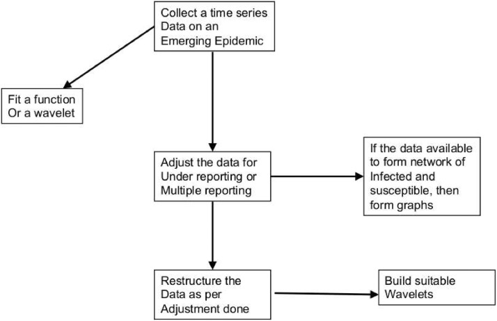
In this study, we are trying to investigate a classical problem in epidemic reporting within a novel framework using harmonic analysis principles. See the flow chart in Fig. 1.1 for an overview of the proposed framework. This study develops methodologies of constructing complete data from partial data using wavelets (by partial data here we mean incomplete data that typically arises under an emerging epidemic, for example, in the novel coronavirus of 2019 or COVID-19). Our approach will be useful in deep learning of very large data structures and creating complete data from partial data. During most of the emerging epidemics, we will be handling only partial data, corresponding full data would be seldom available. The proposed ideas, hence, could be helpful in artificial intelligence (AI) based algorithms to create disease surveillance.

Fig. 1.1.

Flow chart describing verious key steps proposed in epidemic data restructuring and constructing wavelets.

2. Fundamental questions

We are raising here very fundamental questions in epidemic reporting. For example, does an epidemic case reported over time follow any pattern? Or, in any particular situation, does an epidemic reporting pattern have anything to do with the actual epidemic wave? Actual epidemic or a true epidemic wave is the number of all cases (reported and not reported) as a function of time, i.e. it could be seen as a function obtained as discretely plotting the number of infected people reported against time points. Is there any strong or weak association between “epidemic reporting patterns” and “epidemic waves” in general? Suppose we cannot generalize such an association for every epidemic, then will there be any such association for a particular epidemic?

In any epidemic, we can hardly observe the actual (true) epidemic wave, and what we construct as a wave is mostly based on reporting numbers of disease cases. The central questions in which we are interested can be summarized as follows:

• (i)How far the reporting of an epidemic is helping us in accurate prediction of an epidemic, especially if it is an emerging epidemic? how far such an association is clarified (which it is not otherwise) using methods of harmonic analysis?
• (ii)It is seldom that the cases generated in a population are completely detected, so the question that remains unanswered most of the time in a newly emerging epidemic is: Will there be any way to back-calculate and reproduce these numbers lost in detection and, if so, to what extent can we reconstruct accurately an epidemic growth (before control measures are implemented)?

There are other related questions but first we want to view matters from the lens of wavelet/harmonic analysis because we believe there could be some useful light to be shed in this way.

It is always challenging to construct true epidemic waves because population vaccination and control policies depend on understanding the true ground level reality of disease cases. Before we treat wavelets in this new context, we define the Fourier series and Fourier tranform of a function2 .

3. Wavelets

In the past thirty-five years there has developed a new branch of harmonic analysis called wavelet theory—see Meyer and Ryan (1993), Meyer (1998), Hernández and Weiss (1996), Walker (1997), Strichartz (1993), Krantz, 1999, Krantz, Krantz and Labate et al. (2013). Largely based on the ideas of Yves Meyer, wavelet theory replaces the traditional Fourier basis of sine functions and cosine functions with a more flexible and adaptable basis of wavelets. The advantages of wavelets are these:

• (a)The wavelet expansion of a function can be localized both in the time and the space variables;
• (b)The wavelet expansion can be customized to particular applications;
• (c)Because of (b), the wavelet expansion is more accurate than the traditional Fourier expansion and also more rapidly converging.

Wavelet theory has revolutionized the study of image compression, the study of signal processing, and the study of partial differential equations. It will be a powerful new tool in the study of epidemiology, particularly in the analysis of epidemic growth curves.

4. Theoretical strategy

This study will develop methodologies of constructing complete data from partial data using wavelets.

First, we propose to build a true wave of an epidemic (through harmonic analysis set-up and assumptions) that is otherwise unknown directly. Then, by assuming that a fraction of this constructed wave was reported out of a true wave, we will determine how an observed wave appears. These fractions are variables, so we will have several patterns of waves representing one true epidemic wave. We will draw conclusions as to which one of these representations is an ideal candidate for building a true epidemic. There will be some noise in our modeling of the epidemic curve so we will use noise reduction techniques before finalizing a pattern.

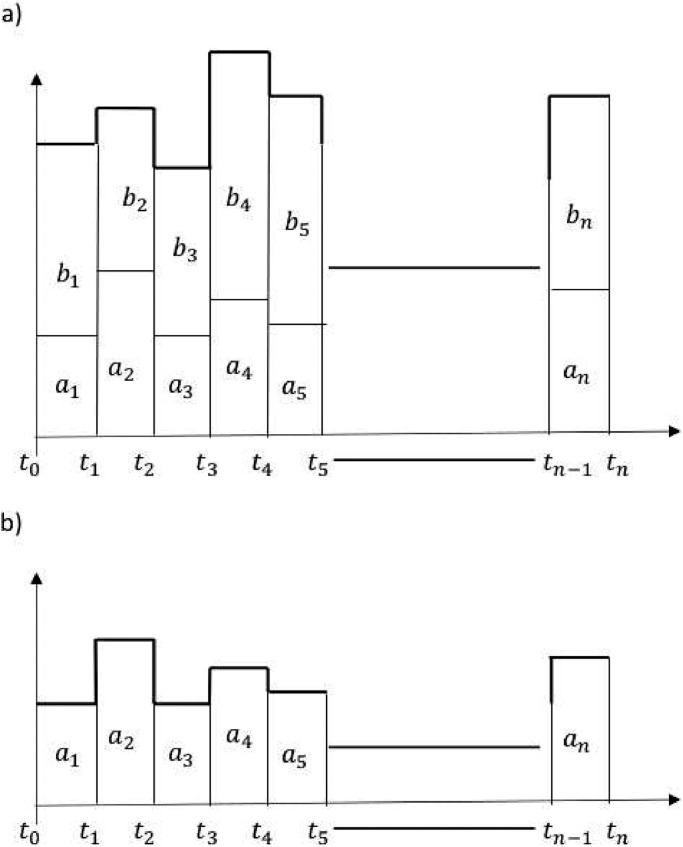
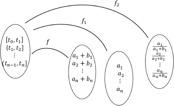
Suppose an epidemic wave was observed within a time interval [t ₀, t_n], where $t_n-t_0$ could be in weeks, months, or years. Suppose that [t ₀, t_n] is partitioned into a set S of sub-intervals $\{[t_0,t_1],(t_1,t_2],\cdots ,(t_{n-1},t_n]\},$ where $t_i-t_{i-1}$ could be in days or weeks depending upon the situation. Let a_i and b_i be the number of cases reported and number of cases that occurred but were not reported, respectively, within the interval $[t_{i-1},t_i]$ for $i=1,2,\cdots ,n.$ Let f be the function whose domain is the set of time intervals $\{[t_{i-1},t_i]\mid \forall i\}$ and whose range is the set $T=\{a_i+b_i\mid i=1,2,\dots ,n\}$ (see Fig. 4.1 ). Here f need not be a one-to-one function because two time intervals within S could have the same number of epidemic cases. Let f ₁ be the function defined as $f_1:\{[t_{i-1},t_i]\mid i=1,2,\dots ,n\}\to A,$ where $A=\{a_i\mid i=1,2,\dots ,n\}$ (see Fig. 4.2 ). We call f ₁ a fractional function of f because it maps each time interval into a corresponding number of reported cases in each of those intervals. The total fraction of reported cases ${\Sigma }_i{a}_i/{\Sigma }_i(a_i+b_i)\in [0,1]$ during [t ₀, t_n] is distributed into n time intervals. Note that

$$\begin{array}{ccc}& & \sum _i\frac{a_i}{a_i+b_i}\hfill \\ & & =\{\begin{array}{c}n\text{if}\text{all}\text{disease}\text{cases}\text{are}\text{reported}\text{during}[t_0,t_n]\\ <n\text{if}\text{any}\text{one}\text{interval}\text{in}S\text{there}\text{exists}\text{under-reporting}\text{of}\\ \text{diseases}\text{cases}\end{array}\hfill \end{array}$$

Fig. 4.1.

a) True epidemic wave and b) Fractional epidemic wave. The a_i values are part of $a_i+b_i$ values for each i. We have newly introduced the phrase fractional epidemic waves in this work. This fractional epidemic waves concept we are using with other ideas explained in this paper to develop new ideas related to fractional wavelets. In a sense, fractional wavelets represent fractions of an overall wavelet. This figure serves as a foundational concept to link the idea of fractional reporting waves with reporting errors.

Fig. 4.2.

Functions of true and fractional epidemic waves based on reported and actual time series epidemic data.

Given that f ₁ is known, the question will be whether we can estimate (or speculate about) f. Once we are able to estimate some form of f, then how can we test for accuracy of the form(s) obtained? We could define another fraction function as

$$f_2:\{[t_{i-1},t_i]\mid i=1,2,\dots ,n\}\to \frac{A}{T}$$

where

$$\frac{A}{T}=\{\frac{a_i}{a_i+b_i}\mid i=1,2,\dots ,n\}$$

and could attempt to develop techniques to estimate (or speculate about) f from f ₂. In Fig. 4.2, the fractional epidemic wave pattern is not fully describing a true epidemic wave pattern. Purely from a fractional epidemic wave, it is not easy to speculate a true epidemic wave pattern. Additional information on b_i values is needed for better prospects in speculation of f.

This work is innovative because wavelets have never before been used to build on partial epidemic information. The wavelets thus built will be retrospectively updated. This will be a new technology to improve reported data and to re-construct epidemic dynamics. These methods, we anticipate, will be innovative for several other medical science applications.

4.1. Generating wavelets from sampled epidemic data:

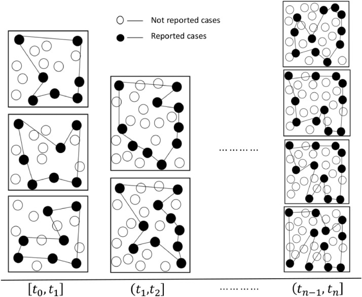
Let us consider the availability of data as per Fig. 4.1 on reported cases. Suppose each point on the y-axis is considered as a sampled point (out of many sets of plausible reported cases at that point). We call it a sample point because we are not sure that the point we obtain at any time intervals [t ₀, t ₁] and $(t_{i-1},t_i]$ for $i=2,3,\dots ,n$ for the reported cases represents a true epidemic curve, which is one of the main assumptions in this paper. The total number of reported cases within a time interval is a combination of cases that were reported to the public health system (see Fig. 4.4). When we know the total number of reported cases within a time interval, then this number could be the result of one of the several combinations of cases reported as shown in Fig. 4.4.

Fig. 4.4.

Total reported cases within an interval of time could be formed from sample cases out of total cases. We drew graphs using black colored filled circles in this Figure to represent total reported cases in a few of the situations out of all possible diseases reporting patterns. The sample point of reported cases represents the total reported cases at each time interval. Hence the size of all graphs at each interval was kept the same. Similarly, the size of graphs between different time intervals is kept different for demonstration purposes only and actual reported cases between different time intervals could be constant or not. During the intervals $[t_{n-1},t_n],$ the number of vertices helped to form graph are constant within each time interval (7 in [t₀, t₁], 10 in (t₁, t₂] but actual structure of the network has changed between various graphs in each time interval.

True number of cases occurring in a population is often unknown, and what we know often is the number of reported cases. Let a_i be the number of reported cases in the i^th time interval, which is to say, the result of one of the several possible combinations of actual cases in the population.

Let T_i be the number of total cases in i^th time interval, and let it be

$$T_i=\{1_i,2_i,\dots ,s_i\},$$

where, s_i is the s^th individual infected in the interval i. Then a_i be the sum of the cases, a number formed with one combination of elements of T_i. There could be several such combinations which could lead to the same value a_i. Hence a_i can be treated as one such sample combination out of many possible combinations. The set of cases which led to form a_i we call here the support of a_i and explain further in the following paragraphs.

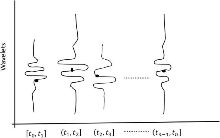
Within each interval, the combination of cases reported is unknown but the total reported cases out of actual disease cases within each interval is fixed (because we will take a single point reference of total reported cases within each interval). These reported cases are a_is in Fig. 4.1. Given that there exists a sampled point within each of the time intervals, and with some support for each of the a_i (say, supp(a_i)), we will construct a wavelet for each time interval [t ₀, t ₁] and $(t_{i-1},t_i]$ for $i=2,3,\dots ,n$. When we say a sample point at a time interval we mean the final combination of cases reported (out of actual cases) that were considered as a final reporting number for that interval. We will use data that was used to get the sample point a_i.

In Fig. 4.4, for the interval [t ₀, t ₁], the arcs connecting each of the black circles (vertices) within each square form a graph. Although the sizes of each of these graphs are the same, i.e. 7, their shapes are different and the sampled point is 7. The sampled point cannot be easily used to represent the shape of the graph unless the location of each node (in this case a physical address or geographical location of each node) is known. One way to construct the support could be from the graph associated with each sample point. Using pairs of information {a_i, supp(a_i)}, we will construct wavelets as shown in Fig. 4.3 . Sampled points within each interval [t ₀, t ₁] and $(t_{i-1},t_i]$ for $i=2,3,\dots ,n$ gives the number of reported cases and supports constructed from the graphs within each of these intervals. Within each square or rectangle in Fig. 4.4, if the size of a graph increases to the maximum possible size (i.e., when all cases are reported), then the information to construct the corresponding support increases.

Fig. 4.3.

Wavelets constructed from sampled reported data with supports. Black color points on wavelets represent sampled points (of total reported cases). Each wavelet is constructed with the pairs of information {a_i, supp(a_i)} available. One of the key technical features is that we are proposing through this figure is to construct wavelets within each interval to quantify the proportion of reporting cases out of actual cases.

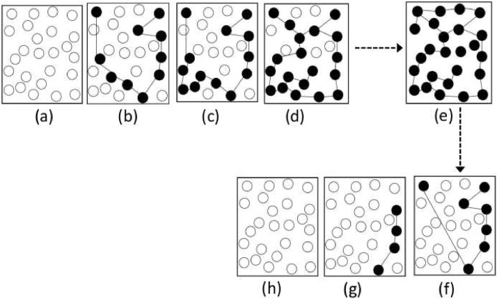
Let G_i be the graph (with n(a_i) vertices and m(a_i) edges) corresponding to a sampled point a_i for the interval $(t_{i-1},t_i]$ and suppose that $G_i^c$ is the graph (with n(T_i) vertices and m(T_i) edges, where T_i is the complete or total infected cases as defined earlier) with all possible reported cases being reported, then, let us say, $G_i\to G_i^c$ (G_i converges to $G_i^c$) for all i. As the reported number of cases increases and it approaches towards the number of complete/actual cases, then the graph G_i would ideally expand (in terms of vertices and edges) towards $G_i^c$. We refer here to this process as convergence. That is, the structure of two graphs G_i and $G_i^c$ get closer. In $G_i^c$ the number of vertices is the number of actual disease cases and the edges are connected between the closest vertices. In reality, $G_i^c$ is not possible to draw because we would not be able to observe all cases. It is challenging to understand beforehand what fraction of the size of $G_i^c$ would be the size of G_i, and this guess could give the speed of convergence to $G_i^c$ from G_i. The actual time steps taken from G_i to $G_i^c$ for each i is not constant. We assume that there will be a finite number of time steps to reach from G_i to $G_i^c.$ Usually c is not constant as well because the error rates vary so we let c ₀ correspond to complete reporting at t ₀, c ₁ at t ₁, and so on up to c_n at t_n. Let $G_i^{t_0}$ be the graph at t ₀ and $G_i^{t_1}$ be the graph at t ₁ and so on. The corresponding sizes of graphs will be $\left|E_i^{t_j}\right|$ for $i=1,2,\dots ,n$ and $j=1,2,\dots ,c_i,$ and

$$\left|E_i^{t_0}\right|<\left|E_i^{t_1}\right|<\dots <\left|E_i^{t_{c_i}}\right|\text{for}\text{each}i.$$ (4.1)

But the inequality

$$\left|E_i^{t_j}\right|<\left|E_l^{t_{j+1}}\right|\text{for}\text{some}i\ne l\text{and}l=1,2,\dots ,n$$

need not hold. The explanation for these inequalities is as follows: graphs within each time interval could converge toward actual disease cases but the size of the graph across various time intervals need not follow any monotonic property because degrees of error in reported cases could vary over time.

For simplicity, let G_i be represented by (V_i, E_i) and $G_i^c$ be represented by $(V_i^c,E_i^c),$ where $(V_i,E_i)=(n\left(a_i\right),m\left(a_i\right)),$ $(V_i^c,E_i^c)=(n\left(T_i\right),m\left(T_i\right))$. As the reporting of diseases cases improves the values of (V_i, E_i) increases so that they become exactly $(V_i^c,E_i^c).$ We denote here as $G_i\to G_i^c$. See Fig. 4.5 .

Fig. 4.5.

Convergence of graph at sample point to graph at complete reporting. From sampled point number of reported cases to the evolution of actual reported cases. This situation arises due to improved epidemic surveillance.

We define ${\max }_j\left|E_i^{t_j}\right|\text{for}i=1,2,\dots ,n$ as the local steady-state values and ${\max }_i\left(\right|E_i^{t_j}\left|\right)$ as global steady-state value. The maximum value of reported cases within the interval i in (4.1) is referred as the local steady-state for the i^th interval. Then, there will be no further improvement of reported cases in that interval. Similarly, global steady-state refers to the maximum number of reported cases for an epidemic across the intervals.

Theorem 1

The size of each graph within $[t_{i-1},t_i)$ could reach local steady-state and the global steady-state is equal to one of the local steady-states.

Proof

Suppose the values $|E_i^{t_j}|\text{for}i=1,2,\dots ,n$ are unique such that

$$\begin{array}{cc}\hfill \left|E_i^{t_{j_1}}\right|\ne & \left|E_i^{t_{j_2}}\right|\text{for}{j}_1\ne j_2\hfill \\ \\ \hfill \left|E_{i_1}^{t_j}\right|\ne & \left|E_{i_2}^{t_j}\right|\text{for}{i}_1\ne i_2.\hfill \end{array}$$

There will be only one value of $|E_i^{t_j}|\text{for}\text{each}i,$ and there will be n such maximum values. One of the n maximum values is the maximum reported cases in one of the n time intervals, so that global steady-state is one of the local steady states. Alternatively, let,

$$\left|E_i^{t_{j_1}}\right|=\left|E_i^{t_{j_2}}\right|\text{for}{j}_1\ne j_2,$$

but $|E_i^{t_{c_i}}|\text{is}\text{unique}\text{for}\text{each}i$ such that

$$\underset{j}{\max }\left|E_i^{t_j}\right|=\left|E_i^{t_{c_i}}\right|.$$

In this situation also, there will be n maximum values and one of the values

$$\{\left|E_1^{t_{c_1}}\right|,\left|E_2^{t_{c_2}}\right|,\dots ,\left|E_n^{t_{c_n}}\right|\}$$

is the global maximum. If

$$\left|E_{i_1}^{t_{c_1}}\right|=\left|E_{i_2}^{t_{c_2}}\right|\text{for}{i}_1\ne i_2,$$

then two local steady-states will be equal to the global steady-state. □

For each i, $|E_i^{t_0}|$ and G_i are associated with reported cases. For any i, when $|E_i^{t_0}|=|E_i^{t_{c_i}}|$ then G_i and $G_i^{t_{c_i}}$ are identical, and this situation refers to complete reporting of disease cases. If $|E_i^{t_0}|=|E_i^{t_{c_i}}|$ for any i, then local steady-state for this i attained at t ₀.

Remark 2

If $|E_i^{t_0}|=|E_i^{t_{c_i}}|$ for each i and ${\max }_i\left(\right|E_i^{t_j}\left|\right)=|E_i^{t_0}|,$ then the global steady-state also attains at t ₀. If $|E_i^{t_0}|\ne |E_i^{t_{c_i}}|$ for all i, then the global stead-state attains at a time greater than t ₀.

When $|E_i^{t_0}|\ne |E_i^{t_{c_i}}|$ for each i, then the global steady-state value could provide information on degree of reporting error to some extent. If $|E_i^{t_0}|=|E_i^{t_{c_i}}|$ for some i, and by chance at this i, the global steady-state occurs then that would not provide any information on the degree of reporting errors, because at several other i values we will have $E_i^{t_0}<\left|E_i^{t_{c_i}}\right|$ and actual total epidemic cases are more than sample epidemic cases.

Above, statements in Proposition 1 and in the Remark 2 will alter when multiple reporting exists in one or more of the time intervals considered. Multiple reporting of cases is usually defined as reporting of a disease case more than once and treating it as more than one event of disease occurrence. When multiple reporting exists at each i, then ${\max }_i\left(\right|E_i^{t_j}\left|\right)\ne |E_i^{t_0}|$ is not the global steady-state. A mixed situation where multiple reporting and under-reporting simultaneously exists within the longer time interval [t ₀, t_n] is treated separately.

With this method, we will develop a series of wavelets.

Given the information to construct Fig. 4.5(a), and the rapidity at which this graph evolves from the Fig. 4.5(a) to the Fig. 4.5(d) (which we might refer to above as support) to attain the Fig. 4.5(d) is known, then, combined with the information stored in Fig. 4.6 , we can then construct Fig. 4.3. Within each of the intervals [t ₀, t ₁] and $(t_{i-1},t_i]$ for $i=2,3,\dots ,n,$ the information of the Figs. 4.5–4.6, will be used to construct a series of wavelets.

Fig. 4.6.

Evolution of reporting of epidemic cases (a) to (e), and returning to disease recovered stage (f) to (h).

In the next few paragraphs, we will describe the philosophy of wavelets and Meyer wavelets. Why Meyer wavelets? Because they are orthogonal, smooth, and rapidly vanishing. Thus they are more stable.

Suppose two functions Ψ(t) and Φ(t) together describe the epidemic wave of a true epidemic, and if pairs of functions{(Ψ_i(t), Φ_i(t))} for $i=1,2,\dots ,n$ represent the epidemic wave of those representing fractions of this true epidemic. Then one of our central ideas is in determining which of these fractional waves (as described in section 4) is closest to the true epidemic. Usually data/information to construct a couple of such fractional wavelets could be observed in an emerging epidemic, say (Ψ_a(t), Φ_a(t))} and (Ψ_b(t), Φ_b(t)), so the first step is to construct these pairs of wavelets. These fractional wavelets are constructed on partial data (partial in the sense that observed data on disease cases in an emerging epidemic is not complete). The question we are attempting is: can we predict (Ψ(t), Φ(t)) from either one of or from both of the fractional wavelets? [Note: There is no terminology of “fractional wavelet” in the literature, but we are calling (Ψ_a(t), Φ_a(t)) and (Ψ_b(t), Φ_b(t)) the fractional wavelets]. For this, let us define Meyer wavelets which are readily available and could be a good first step to start with to explain our epidemic situation. We define the Meyer wavelet and briefly describe them below:

The Meyer wavelet is an orthogonal wavelet created by Yves Meyer. It is a continuous wavelet, and has been applied to the study of adaptive filters, random fields, and multi-fault classification.

Definition 3

The Meyer wavelet is an infinitely differentiable function that is defined in the frequency domain in terms of a function ν as follows:

$$\Psi \left(\omega \right)=\{\begin{array}{cc}\begin{array}{c}{\displaystyle \frac{1}{\sqrt{2\pi }}\sin \left(\frac{\pi }{2}\nu (\frac{3\left|\omega \right|}{2\pi }-1)\right)e^{j\omega /2}}\hfill \\ {\displaystyle \frac{1}{\sqrt{2\pi }}\cos \left(\frac{\pi }{2}\nu (\frac{3\left|\omega \right|}{2\pi }-1)\right)e^{j\omega /2}}\hfill \\ 0\hfill \end{array}\hfill & \begin{array}{cc}\begin{array}{c}\text{if}\\ \text{if}\\ \text{if}\end{array}& \begin{array}{c}2\pi /3<\left|\omega \right|<4\pi /3\hfill \\ 4\pi /3<\left|\omega \right|<8\pi /3\hfill \\ \text{otherwise.}\hfill \end{array}\end{array}\hfill \end{array}$$

Here

$$\nu \left(x\right)=\{\begin{array}{cc}\begin{array}{c}0\hfill \\ x\hfill \\ 1\hfill \end{array}\hfill & \begin{array}{cc}\begin{array}{c}\text{if}\\ \text{if}\\ \text{if}\end{array}\hfill & \begin{array}{c}x<0\hfill \\ 0<x<1\hfill \\ x>1.\hfill \end{array}\hfill \end{array}\hfill \end{array}$$

There are other possible choices for ν.

The Meyer scaling function is given by

$$\Phi \left(\omega \right)=\{\begin{array}{cc}\begin{array}{c}{\displaystyle \frac{1}{\sqrt{2\pi }}}\\ {\displaystyle \frac{1}{\sqrt{2\pi }}\cos \left(\frac{\pi }{2}\nu (\frac{3\left|\omega \right|}{2\pi }-1)\right)}\\ 0\end{array}\hfill & \begin{array}{cc}\begin{array}{c}\text{if}\\ \text{if}\\ \text{if}\end{array}& \begin{array}{c}\left|\omega \right|<2\pi /3\hfill \\ 2\pi /3<\left|\omega \right|<4\pi /3\hfill \\ \text{otherwise.}\hfill \end{array}\end{array}\hfill \end{array}$$

Of course it holds, as usual, that

$$\underset{k}{\Sigma }{\left|\widehat{\Phi (\omega +2\pi k)}\right|}^2=\frac{1}{2\pi }$$

and

$$\widehat{\Phi \left(\omega \right)}=m_0(\omega /2)\widehat{\Phi (\omega /2)}$$

for some $2\pi -$periodic m ₀(ω/2). Finally,

$$\Psi \left(\omega \right)=e^{i\omega /2}\overline{m_0(\omega /2+\pi )}\widehat{\Phi }(\omega /2)=e^{i\omega /2}\sum _k\overline{\widehat{\Phi }(\omega +2\pi (2k+1\left)\right)}\widehat{\Phi }(\omega /2)=e^{i\omega /2}(\widehat{\Phi }(\omega +2\pi )+\widehat{\Phi }(\omega -2\pi ))\widehat{\Phi }(\omega /2).$$

It turns out that the wavelets

$${\Psi }_{j,k}\left(x\right)=2^{j/2}\Psi (2^{j}x-k)$$

form an orthonormal basis for the square integrable functions on the real line.

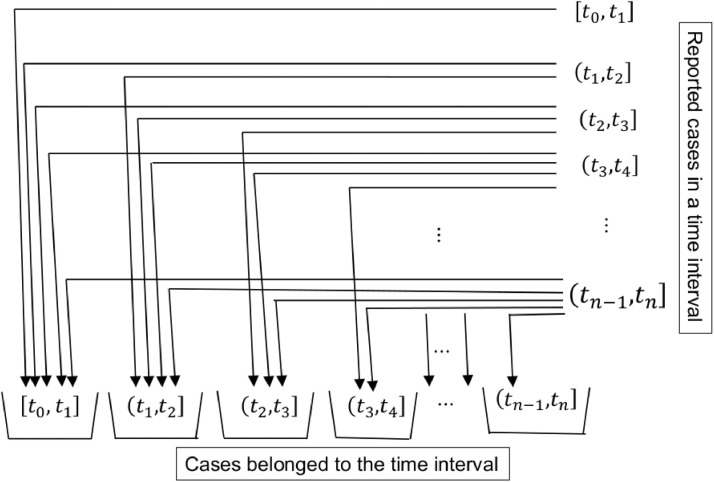
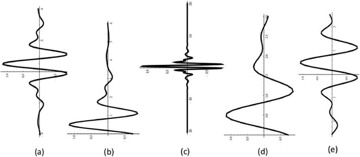
One proposition that could be formed is “if a wavelet is constructed on the partial data of a particular series of events in a population, then this wavelet can not be fully compared with a wavelet constructed from the full data series of all events in the same population.” Building a measure associated with these two wavelets is interesting, and there could be several such measures based on the level of completeness in the data. Because we are dealing with true versus reported disease cases, this measure (a set of points each representing a distance between true and observed cases) could be termed the error in the reporting of disease cases. These kinds of measures will be very helpful (such measures after further filtration can be useful for practical epidemiologists). Instead of constructing wavelets for the overall epidemic duration, we will construct wavelets within intervals [t ₀, t ₁] and $(t_{i-1},t_i]$ for $i=2,3,\dots ,n$ described as in Fig. 4.3. As the reported cases within an interval improve, described as in Fig. 4.5, the wavelet configuration improves. Each of the fractional wavelets obtained from partial data will be updated using the information shown in Fig. 4.7 . Meyer wavelets for various equally spaced intervals are demonstrated in Fig. 4.8 .

Fig. 4.7.

Distribution of reported cases into present time interval and to past time intervals. Reported cases found in a time interval in the column are distributed into respective bins of a time interval as shown through arrows.

Fig. 4.8.

Meyer wavelets of order 3 for various situations for equally spaced interval of (a) [-4,4], (b) [0,6], (c) [-20,20,], (d) [0,3], (e) with order 10 for [-2.5, 2.5].

4.1.1. Computation

Suppose a sample point is obtained as explained in the Section 4.1 for an interval $(t_{i-1},t_i]$. An improvement of reported cases is ascertained from the data obtained in the subsequent time intervals. One way to update this is from future epidemic cases that were infected and/or diagnosed for the period $(t_{i-1},t_i]$ but made available during any of the intervals $(t_i,t_{i+1}]$ for $i=2,3,\dots ,n-1.$ That is, the sum of the epidemic cases that were reported during $(t_{i-1},t_i]$ and those reported during each of the future time intervals $(t_i,t_{i+1}]$ for $i=2,3,\dots ,n-1$ and that belong to the interval $(t_{i-1},t_i]$ will be treated as an improved number of reported cases for the interval $(t_{i-1},t_i]$. We will update the reported number of cases in a previous interval from the future available reported cases that were associated with the previous time interval. Hence the evolution of the data for the interval $(t_{i-1},t_i]$ can be used to construct graphs as shown in Fig. 4.5. Since this evolution is assumed to be observed for a long period, it is also assumed that G_i will be approximately convergent to $G_i^c.$ As an epidemic progresses, we will update the intervals $(t_{i-1},t_i]$ with newly available information during $(t_i,t_{i+1}]$ and as i approaches n then those intervals nearby to n will have less of a chance of evolution or less chance of up-gradation (due to a truncation effect). Once the reported numbers are complete, we will similarly study the recovery stage of an epidemic and hence collect the data to compute Fig. 4.6. Accumulation of old cases in new intervals distributed back to the respective time intervals is schematically described in Fig. 4.7. This procedure will update the reported cases in the past as long as at least one reported case observed in the present time interval belongs to one of the past time intervals. Based on the location of the reported cases the graphs constructed will be updated as well. Hence for each present time interval that we observe a reported case that belongs to one of the past time intervals, the fractional wavelets will become graphically closer to the complete (or true) wavelet for that time interval.

5. Numerical examples

To demonstrate our method, we have constructed two numerical toy examples. We have generated non-uniform random positive integers of a_i values for $i=1,2,\dots ,12.$ The a_i values generated are in Table 1 .

Table 1.

Numerical values of a_i for $i=1,2,\dots ,12.$

$a_1=83,$

$a_2=64,$

$a_3=87,$

$a_4=85,$

$a_5=90,$

$a_6=60,$

$a_7=62,$

$a_8=55,$

$a_9=40,$

$a_{10}=20,$

$a_{11}=45,$

$a_{12}=31$

A fraction of a_i for i > 1 was assumed to have occurred prior to the i^th time interval but are reported in the i^th time interval, and we have adjusted excess values of a_i as per the formula below:

$$a_i=a_i^{*}+a_1^{*}+a_2^{*}+\cdots +a_{i-1}^{*},$$ (5.1)

where $a_i^{*}$ is the number of reported cases in the i^th time interval which belonged to the i^th time interval and $a_j^{*}$ for j < i is the reported cases in the i^th time interval which belonged to one or more of the j^th time interval for $j=1,2,\dots ,i-1.$ Using the below formula (5.1), we will retrospectively adjust a ₂, $a_3,\dots ,a_{12}$ values by using below equations:

$$\begin{array}{ccccc}{a}_2& =& a_2^{*}& +& a_1^{*}\\ a_3& =& a_3^{*}& +& a_2^{*}& +& a_1^{*}\\ ⋮& & ⋮\\ a_{12}& =& a_{12}^{*}& +& a_1^{*}& +& a_2^{*}& +\cdots & a_{11}^{*}.\end{array}$$ (5.2)

The values of reported cases in the expression in (5.2) in the i^th time interval are numerically computed using the set of equations in (5.3) (Table 2 )

$$\begin{array}{ccccc}{a}_2& =& a_2{\varphi }_{22}& +& a_1{\varphi }_{21}\\ a_3& =& a_3{\varphi }_{33}& +& a_1{\varphi }_{31}& +& a_2{\varphi }_{32}\\ ⋮& & ⋮\\ a_i& =& a_i{\varphi }_{ii}& +& a_1{\varphi }_{i1}& +& a_2{\varphi }_{i2}& +\cdots & a_{1-1}{\varphi }_{i(i-1)}.\end{array}$$ (5.3)

Example 4

In (5.3), ${\varphi }_{22}+{\varphi }_{21}=1$ and ϕ ₂₂ is a random fraction in [0.6,0.95], i.e. among the reported cases in the 2nd time interval 60 % to 95 % belong to the same time interval and $(1-{\varphi }_{22})$ fraction belong to the 1st time interval. The interval [0.6,0.95] is arbitrary and it can be changed to a different range of fractions. Again, assume ${\varphi }_{33}+{\varphi }_{31}+{\varphi }_{32}=1$ and ϕ ₃₃ is picked randomly to take a value within the interval [0.6,0.95]. Once ϕ ₃₃ is fixed, ϕ ₃₁ is assumed to take a value that is picked randomly from the interval $[0,(1-{\varphi }_{33})]$. The number ϕ ₃₂ is obtained as $1-{\varphi }_{33}-{\varphi }_{31}.$

Table 2.

ϕ values (set 1).

${\varphi }_{22}=0.73,$	${\varphi }_{21}=0.27$
${\varphi }_{33}=0.72,$	${\varphi }_{31}=0.26,$	${\varphi }_{32}=0.02$
${\varphi }_{44}=0.94,$	${\varphi }_{41}=0.05,$	${\varphi }_{43}=0,$	${\varphi }_{41}=0.01$
${\varphi }_{55}=0.92,$	${\varphi }_{51}=0,$	${\varphi }_{52}=0.07,$	${\varphi }_{53}=0,$	${\varphi }_{54}=0.01$
${\varphi }_{66}=0.88,$	${\varphi }_{61}=0.04,$	${\varphi }_{62}=0.07,$	${\varphi }_{63}=0.01,$	${\varphi }_{64}=0,$	${\varphi }_{65}=0$
${\varphi }_{77}=0.77,$	${\varphi }_{71}=0.05,$	${\varphi }_{72}=0.14,$	${\varphi }_{73}=0.04,$	${\varphi }_{74}=0,$	${\varphi }_{75}=0,$
${\varphi }_{76}=0$
${\varphi }_{88}=0.63,$	${\varphi }_{81}=0.18,$	${\varphi }_{82}=0.04,$	${\varphi }_{83}=0.14,$	${\varphi }_{84}=0.01,$	${\varphi }_{85}=0,$
${\varphi }_{86}=0,$	${\varphi }_{87}=0$
${\varphi }_{99}=0.83,$	${\varphi }_{91}=0.12,$	${\varphi }_{92}=0.01,$	${\varphi }_{93}=0.02,$	${\varphi }_{94}=0,$	${\varphi }_{95}=0,$
${\varphi }_{96}=0,$	${\varphi }_{97}=0,$	${\varphi }_{98}=0.01$
${\varphi }_{\left(10\right)\left(10\right)}=0.79,$	${\varphi }_{\left(10\right)1}=0.08,$	${\varphi }_{\left(10\right)2}=0.04,$	${\varphi }_{\left(10\right)3}=0.01,$	${\varphi }_{\left(10\right)4}=0.04,$	${\varphi }_{\left(10\right)5}=0,$
${\varphi }_{\left(10\right)6}=0.02,$	${\varphi }_{\left(10\right)7}=0,$	${\varphi }_{\left(10\right)8}=0.01,$	${\varphi }_{\left(10\right)9}=0.01$
${\varphi }_{\left(11\right)\left(11\right)}=0.70,$	${\varphi }_{\left(11\right)1}=0.18,$	${\varphi }_{\left(11\right)2}=0.06,$	${\varphi }_{\left(11\right)3}=0,$	${\varphi }_{\left(11\right)4}=0.05,$	${\varphi }_{\left(11\right)5}=0,$
${\varphi }_{\left(11\right)6}=0,$	${\varphi }_{\left(11\right)7}=0.01,$	${\varphi }_{\left(11\right)8}=0,$	${\varphi }_{\left(11\right)9}=0,$	${\varphi }_{\left(11\right)\left(10\right)}=0$
${\varphi }_{\left(12\right)\left(12\right)}=0.91,$	${\varphi }_{\left(12\right)1}=0.04,$	${\varphi }_{\left(12\right)2}=0.01,$	${\varphi }_{\left(12\right)3}=0.02,$	${\varphi }_{\left(12\right)4}=0,$	${\varphi }_{\left(12\right)5}=0.02,$
${\varphi }_{\left(12\right)6}=0,$	${\varphi }_{\left(12\right)7}=0,$	${\varphi }_{\left(12\right)8}=0,$	${\varphi }_{\left(12\right)9}=0,$	${\varphi }_{\left(12\right)\left(10\right)}=0,$	${\varphi }_{\left(12\right)\left(11\right)}=0$

In a similar way, ${\varphi }_{ii}+{\varphi }_{i1}+\cdots +{\varphi }_{i(i-1)}$ is assumed to be 1 and ϕ_ii is picked randomly to take a value within the interval [0.6,0.95]. Once ϕ_ii is fixed, ϕ _i1 is assumed to take a value that is picked randomly from the interval $[0,(1-{\varphi }_{ii})],$ ϕ _i2 is assumed to take a value that is picked randomly from the interval $[0,(1-{\varphi }_{ii}-{\varphi }_{i1})],$ and so on ${\varphi }_{i(i-2)}$ is assumed to take a value that is picked randomly from the interval

$$[0,(1-{\varphi }_{ii}-{\varphi }_{i1}-\cdots -{\varphi }_{i(i-3)})].$$

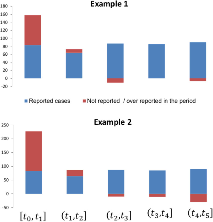
Finally, ${\varphi }_{i(i-1)}$ is obtained as $1-{\varphi }_{ii}-{\varphi }_{i1}-\cdots -{\varphi }_{i(i-2)}.$ All the random values picked are expanded to two decimal places. In case due to rounding of numbers to nearest integer causes a situation such that $a_i<{\sum }_{k=1}^i{a}_i{\varphi }_{ik},$ then the excess value is discounted from the value already computed for a_iϕ_ii to make $a_i={\sum }_{k=1}^i{a}_i{\varphi }_{ik}.$ If the already-computed value for $a_i{\varphi }_{ii}=0,$ then the discount is done from a_iϕ _i1, and if $a_i{\varphi }_{i1}=0,$ then discounting will be done from a_iϕ _i2, and it will be repeated until the discounting of excess value is done (Fig. 5.1 ).

Fig. 5.1.

Reported cases and adjusted cases for the first five time intervals. Example 1 and Example 2 are drawn from the reported data in the Table 1 and in the Table 4.

Using the ϕ values and expressions in (5.3), we partition reported values in each interval into cases: those belong to the same interval and those belong to previous intervals. See Table 3 .

Example 5

We have constructed our second toy example by considering a different interval [0.5,0.8] in which to pick ϕ_ii values for $i=1,2,\dots ,12$. We have repeated the procedure explained in Example 4 to obtain the ϕ value table, partition values of a_i, and adjusted values of a_i. The results are shown in Table 4 .

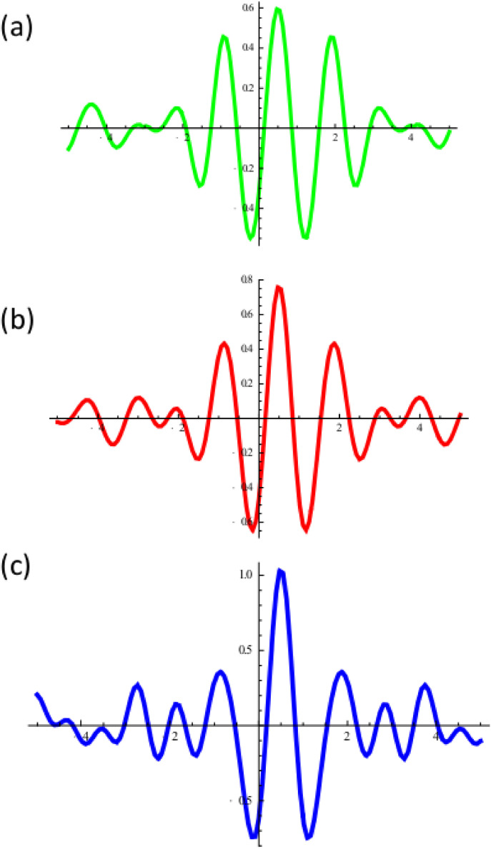
Meyer wavelet of various order were computed based on the number of cases reported as a proportion of the total adjusted cases in Example 2, Table 4. These are in Fig. 5.2 . Mayer wavelets are smooth and rapidly decreasing. The basis made up of Meyer wavelets is unconditional. The wavelets act robustly in our situation and hence the pictorial differences between the three wavelets of Fig. 5.2 are minimal. Yet the differences in patterns is definitely present because of the order of the various wavelets. The a_i values are taken from each of the numerical examples or a real epidemic data collected. They can be combined with the network of people who are connected with each of the disease cases to construct graphs for the interval i for $i=1,2,3,\dots ,12.$ We are proposing that such graphs will help in assisting measures of controlling the spread.

Table 3.

Partitioning of a_i values due to adjustment of reported cases retrospectively (set 1).

Cases belonged to ti below means the time interval beginning from $[t_i,t_{i+1})$.
Reported cases	t0	t1	t2	t3	t4	t5	t6	t7	t8	t9	t10	t11
in ith interval
$a_1=83$	83
$a_2=64$	17	47
$a_3=87$	23	1	63
$a_4=85$	4	0	1	80
$a_5=90$	0	6	0	1	83
$a_6=60$	2	4	1	0	0	53
$a_7=62$	3	9	2	0	0	0	48
$a_8=55$	10	2	8	0	0	0	0	35
$a_9=40$	5	0	1	0	0	0	0	1	33
$a_{10}=20$	2	1	0	1	0	0	0	0	0	16
$a_{11}=45$	8	3	0	2	0	0	0	0	0	0	32
$a_{12}=31$	1	0	0	0	0	0	0	0	0	0	2	28

Table 4.

Adjusted a_i values retrospectively from the prospective data obtained in Example 4 and in Example 5.

Example 1 data
$a_1=158,$	$a_2=73,$	$a_3=76,$	$a_4=85,$	$a_5=83,$	$a_6=53,$	$a_7=48,$	$a_8=36,$	$a_9=33,$
$a_{10}=16,$	$a_{11}=34,$	$a_{12}=28$
Example 2 data
$a_1=227,$	$a_2=86,$	$a_3=77,$	$a_4=74,$	$a_5=60,$	$a_6=41,$	$a_7=32,$	$a_8=44,$	$a_9=24,$
$a_{10}=12,$	$a_{11}=29,$	$a_{12}=18$

Fig. 5.2.

Meyer wavelets constructed on reported and adjusted disease cases. (a) by treating adjusted value of reported cases in Example 2 as 100% reported (order 100), (b) by treating 90% of the disease are reported (order 90), (c) by treating 40% of the original (adjusted) values are reported (order 40).

6. Discussion

We provide a group of epidemic growth scenarios inspired by the harmonic analysis set-up. A couple of scenarios from this could represent true epidemic growth curves. With this, we will be in a position to assess the level of under-reporting in a particular epidemic. So the strategy we are proposing could be beneficial in not only building a true epidemic but also assessing the level of reporting error in an epidemic. We provide the true epidemic with noise to illustrate our claim (Table 5 ).

Table 5.

ϕ values (set 2).

${\varphi }_{22}=0.71,$	${\varphi }_{21}=0.29$
${\varphi }_{33}=0.57,$	${\varphi }_{31}=0.23,$	${\varphi }_{32}=0.20$
${\varphi }_{44}=0.62,$	${\varphi }_{41}=0.28,$	${\varphi }_{43}=0.07,$	${\varphi }_{41}=0.03$
${\varphi }_{55}=0.66,$	${\varphi }_{51}=0.04,$	${\varphi }_{52}=0.01,$	${\varphi }_{53}=0.11,$	${\varphi }_{54}=0.18$
${\varphi }_{66}=0.67,$	${\varphi }_{61}=0.28,$	${\varphi }_{62}=0.03,$	${\varphi }_{63}=0.02,$	${\varphi }_{64}=0,$	${\varphi }_{65}=0$
${\varphi }_{77}=0.5,$	${\varphi }_{71}=0.46,$	${\varphi }_{72}=0.01,$	${\varphi }_{73}=0,$	${\varphi }_{74}=0.01,$	${\varphi }_{75}=0.01,$
${\varphi }_{76}=0.01$
${\varphi }_{88}=0.79,$	${\varphi }_{81}=0,$	${\varphi }_{82}=0.11,$	${\varphi }_{83}=0.08,$	${\varphi }_{84}=0.02,$	${\varphi }_{85}=0,$
${\varphi }_{86}=0,$	${\varphi }_{87}=0$
${\varphi }_{99}=0.6,$	${\varphi }_{91}=0.31,$	${\varphi }_{92}=0.06,$	${\varphi }_{93}=0.02,$	${\varphi }_{94}=0.01,$	${\varphi }_{95}=0,$
${\varphi }_{96}=0,$	${\varphi }_{97}=0,$	${\varphi }_{98}=0$
${\varphi }_{\left(10\right)\left(10\right)}=0.65,$	${\varphi }_{\left(10\right)1}=0.14,$	${\varphi }_{\left(10\right)2}=0.08,$	${\varphi }_{\left(10\right)3}=0.13,$	${\varphi }_{\left(10\right)4}=0,$	${\varphi }_{\left(10\right)5}=0,$
${\varphi }_{\left(10\right)6}=0,$	${\varphi }_{\left(10\right)7}=0,$	${\varphi }_{\left(10\right)8}=0,$	${\varphi }_{\left(10\right)9}=0$
${\varphi }_{\left(11\right)\left(11\right)}=0.62,$	${\varphi }_{\left(11\right)1}=0.30,$	${\varphi }_{\left(11\right)2}=0.02,$	${\varphi }_{\left(11\right)3}=0,$	${\varphi }_{\left(11\right)4}=0.04,$	${\varphi }_{\left(11\right)5}=0.01,$
${\varphi }_{\left(11\right)6}=0.01,$	${\varphi }_{\left(11\right)7}=0,$	${\varphi }_{\left(11\right)8}=0,$	${\varphi }_{\left(11\right)9}=0,$	${\varphi }_{\left(11\right)\left(10\right)}=0$
${\varphi }_{\left(12\right)\left(12\right)}=0.59,$	${\varphi }_{\left(12\right)1}=0.08,$	${\varphi }_{\left(12\right)2}=0.09,$	${\varphi }_{\left(12\right)3}=0.2,$	${\varphi }_{\left(12\right)4}=0.03,$	${\varphi }_{\left(12\right)5}=0,$
${\varphi }_{\left(12\right)6}=0,$	${\varphi }_{\left(12\right)7}=0,$	${\varphi }_{\left(12\right)8}=0,$	${\varphi }_{\left(12\right)9}=0,$	${\varphi }_{\left(12\right)\left(10\right)}=0,$	${\varphi }_{\left(12\right)\left(11\right)}=0.01$

In addition to the gain in construction of a true epidemic, we also propose new methods that blend harmonic analysis with dynamical systems and sampling strategy. In this way, harmonic analysis is used to bridge the gap between unknown and known information in disease epidemiology. Suppose we determine one of the fractional wavelets, say (Ψ_a(t), Φ_a(t)), is closest to the true wavelet (conceptually based on actual disease cases in the population) ; then finding a measure which is the difference of plots between two wavelets (Ψ_a(t), Φ_a(t)) and (Ψ(t), Φ(t)) will complete the mapping of the epidemic at time t. However determining which one of the fractions (Ψ_i(t), Φ_i(t)) is closest to the true one is not so easy. But if there are no significant multiple reporting of disease cases then the largest fractional wavelet could be assumed to be the one with shortest measure (Table 6 ).

Table 6.

Partitioning of a_i values due to adjustment of reported cases retrospectively (set 2).

Cases belonged to ti below means the time interval beginning from $[t_i,t_{i+1})$.
Reported cases	t0	t1	t2	t3	t4	t5	t6	t7	t8	t9	t10	t11
in hith interval
$a_1=83$	83
$a_2=64$	19	45
$a_3=87$	22	17	50
$a_4=85$	24	6	2	53
$a_5=90$	4	1	10	16	59
$a_6=60$	17	2	1	0	0	40
$a_7=62$	29	1	0	1	1	1	31
$a_8=55$	0	6	4	1	0	0	1	43
$a_9=40$	12	2	1	0	0	0	0	1	24
$a_{10}=20$	3	2	3	0	0	0	0	0	0	12
$a_{11}=45$	14	1	0	2	0	0	0	0	0	0	28
$a_{12}=31$	2	3	6	1	0	0	0	0	0	0	1	18

We have argued how various combinations of partial data can be used for discrete constructions which in turn form a piece of supporting information to construct wavelets. These two aspects make our proposed work very innovative. In summary, what we are trying to develop through this paper is, given that we have partial data of an event (here we mean event of reporting of disease cases), we will construct the complete event data. Wavelets, in this work, are occupying a key role in the processing of built-up or accumulated data to build complete event data. The event here is the reported number of cases in a time interval and these reported cases represent only a partial number of actual epidemic cases. Through this paper, we demonstrated a method of improving partial data to be close to data that could be complete. How we plan to update our data reported in an interval and bring it closer to the actual number of disease cases is described in this paper.

This exploration will assist in better visualization of any emerging epidemic spread in a more realistic sense. We also believe that our methods could provide additional tools for those epidemic modelers who frequently use modeling tools such as ODE and PDE, to begin with. We are not only looking for academic development through this project but, also a clear non-trivial body of techniques for applications of harmonic analysis that has never been seen before in terms of developing epidemic analysis. We plan to come up with some interesting insights on how to construct wavelets for medical applications. The bottom line is that we will be able to help public health planners for better management and courses of action during emerging epidemics. The kind of analysis we present here to fill missing pieces of epidemic reporting information can be applied to other areas, for example, constructing total rhythm of a heartbeat from partial information, etc.

We have identified a gap in the methods of understanding true epidemic growth and spread and tried to address this lacuna by proposing a novel method. We are proposing through this study that wavelets could offer a road map closer to finding a practical solution (we are aware that a perfect solution is impossible by any method because some of the disease cases in any situation are never reported). Technical aspects of the storyline depending on the construction of discrete graphs and fractional wavelets. Fractional wavelets are newly introduced to the literature through this study. A solution through wavelets is also not trivial because there is no ready-made set of wavelets available which will offer a timely road-map. So we have introduced a novel strategy. Hence we argue that our approach will help us to come closer to our aims of understanding epidemics in a more accurate and timely fashion. As a bi-product, we can develop techniques for data scientists to analyze disease surveillance.

7. Questions still remain

Within what period we can generate a true epidemic from its emergence using the harmonic analysis set-up? Can we predict the full picture of an epidemic from only partial data? Can we measure the validity and the accuracy of an epidemic growth curve? Can we conduct a timely analysis of the preliminary data using the proposed techniques ?

Funding

None.

CRediT authorship contribution statement

Steven G. Krantz: Conceptualization, Methodology, Validation, Investigation. Peter Polyakov: Writing - review & editing. Arni S.R. Srinivasa Rao: Conceptualization, Data curation, Formal analysis, Methodology, Validation, Investigation, Project administration, Software, Supervision, Visualization, Writing - original draft.

Declaration of Competing Interest

None.

References

- Anderson R.M., Grenfell B.T., May R.M. Oscillatory fluctuations in the incidence of infectious disease and the impact of vaccination: time series analysis. J. Hyg. 1984;93:587–608. doi: 10.1017/s0022172400065177. [DOI] [PMC free article] [PubMed] [Google Scholar]
- Anderson R.M., May R.M. Oxford Univ. Press; Oxford: 1991. Infectious Diseases of Humans: Dynamics and Control. [Google Scholar]
- Bartlett M.S. Proceedings of the Third Berkeley Symposium on Mathematical Statistics and Probability, Volume 4: Contributions to Biology and Problems of Health, 81–109, 1956. University of California Press; Berkeley, Calif: 1956. Deterministic and tochastic odels for ecurrent pidemics. [Google Scholar]; https://projecteuclid.org/euclid.bsmsp/1200502549.
- Bartlett M.S. Measles periodicity and community size. J. R. Stat. Soc. A. 1957;120(1957):48–70. [Google Scholar]
- Bauch C.T. Vol. 1945. Springer Verlag; 2008. The role of mathematical models in explaining recurrent outbreaks of infectious childhood diseases’. in: ‘mathematical epidemiology. (Lecture Notes in Mathematics, Mathematical Biosciences Subseries). [Google Scholar]
- Bauch C.T., Earn D.J.D. Proceedings of the Royal Society of London B. Vol. 270. 2003. Transients and attractors in epidemics; pp. 1573–1578. [DOI] [PMC free article] [PubMed] [Google Scholar]
- Bauch C.T., Earn D.J.D. Interepidemic intervals in forced and unforced SEIR models. In: Ruan S., Wolkowicz G., Wu J., editors. Dynamical Systems and Their Applications in Biology. Vol. 36. Fields Institute Communications; 2003. pp. 33–44. [Google Scholar]
- Cazelles B., Cazelles K., Chavez M. Wavelet analysis in ecology and epidemiology: impact of statistical tests. J. R. Soc. Interface. 2014;11:20130585. doi: 10.1098/rsif.2013.0585. [DOI] [PMC free article] [PubMed] [Google Scholar]
- Earn D., Rohani P., Grenfell B.T. Spatial dynamics and persistence in ecology and epidemiology. Proc. R. Soc. Lond. B. 1998;265:7–10. doi: 10.1098/rspb.1998.0256. [DOI] [PMC free article] [PubMed] [Google Scholar]
- Grenfell B.T., Bjø rnstad O.N., Kappey J. Travelling waves and spatial hierarchies in measles epidemics. Nature. 2001;414:716–723. doi: 10.1038/414716a. [DOI] [PubMed] [Google Scholar]
- Grenfell B.T., Bolker B.M., Kleczkowski A. Seasonality and extinction in chaotic metapopulations. Proc. R. Soc. Lond. B. 1995;259:97–103. [Google Scholar]
- Hernández E., Weiss G. CRC Press; LLC: 1996. A First Course on Wavelets. [Google Scholar]
- Krantz S.G. Vol. 27. Mathematical Association of America; Washington: 1999. A Panorama of Harmonic Analysis. (Carus Mathematical Monographs). [Google Scholar]
- Krantz, S. G., 2019. Fourier analysis and differential equations with wavelets and applications. Book in preparation.
- Labate D., Weiss G., Wilson E. Wavelets. Notices Amer. Math. Soc. 2013;60(2013):66–76. [Google Scholar]
- Meyer Y. Vol. 9. American Mathematical Society; Providence, RI: 1998. Wavelets, Vibrations and Scalings. With a preface in French by the author. (CRM Monograph Series). [Google Scholar]
- Meyer Y., Ryan R.D. Society for Industrial and Applied Mathematics; Philadelphia: 1993. Wavelets: Algorithms and Applications. [Google Scholar]
- Rao A.S.R.S. Understanding theoretically the impact of reporting of disease cases in epidemiology. J. Theoret. Biol. 2012;302(2012):89–95. doi: 10.1016/j.jtbi.2012.02.026. [DOI] [PubMed] [Google Scholar]
- Soper H.E. The interpretation of periodicity in disease prevalence. J. Roy. Stat. Soc, Ser. A. 1929;92:34–61. [Google Scholar]
- Strichartz R.S. How to make wavelets. Am. Math. Mon. 1993;100(6):539–556. [Google Scholar]
- Walker J.S. Fourier analysis and wavelet analysis. Notices Amer. Math. Soc. 1997;44(6):658–670. [Google Scholar]