LIGHTCURVE ANALYSIS OF ASTEROIDS OBSERVED BY KMTNET-SAAO

Abstract

Observations from the South Africa node of the Korea Microlensing Telescope Network (KMTNe-SAAO) were analyzed using the open source Photometry Pipeline (PP). PP can identify serendipitously observed asteroids in the observation fields which led to the extraction of 53 asteroid lightcurves. Rotational periods for 49 of these targets could be determined and are presented here

The primary objective of the Korea Microlensing Telescope Network (KMTNet; Kim et al., 2016) is to search for extrasolar planets. The network, which consists of three 1.6-m telescopes located in South Africa, Korea, and Chile, was designed to provide continuous coverage of the galactic center looking for gravitational microlensing phenomenon.

The asteroid observations presented here were performed over three nights (2018 Jan 9–11) with the 1.6-m telescope in South Africa. The observed fields were originally intended for an unrelated study but due to the large 2×2 deg field of view, covered by four 9k×9k CCDs, untargeted asteroids were bound to appear in the images. For these observations 53 asteroids were identified in the observation fields.

This was done by using the Photometry Pipeline (PP; Mommert, 2017) which uses the IMCCE SkyBoT service (Berthier et al., 2006) to identify serendipitously observed asteroids. All observations were performed using the Rc filter with 120-second exposures taken at a 190-second cadence. Based on work by Pravec et al. (2000), the 120 sec exposures would allow finding periods for asteroids where P > 0.178 hr (~ 10.7 min).

The 53 asteroid lightcurves are presented here along with rotational periods for 49 of those targets. A similar analysis using PP on KMTNet-SAAO data (with the addition of V-R and V-I colors) for approximately 1000 objects were published by Erasmus et al. (2018).

Data Manipulation and Analysis

The photometry data extracted from the KMTNet-SAAO data were converted by Erasmus to ALCDEF-compatible files (http://alcdef.org). The format goes beyond simple JD/magnitude pairs to include metadata about the object, the system used to make observations, the filter used, etc. so that the end-user can use the data correctly to confirm results derived from the original dataset or independent analysis for other purposes.

The ALCDEF files were imported into MPO Canopus, which was used for period analysis and lightcurve generation. MPO Canopus incorporates the FALC Fourier analysis algorithm developed by Harris (Harris et al., 1989). The initial search used 4^th order Fourier analysis in a range from 2 to 27 hours in steps of 0.01 hr. At first, the raw data were plotted in order to find any obvious outliers since the photometry pipeline did not automatically scrub the data. A quick review of the raw plots indicated if the initial search parameters needed to be revised.

In the Fourier analysis, the general principle is to find a minimum RMS fit of the model lightcurve versus the data. The algorithm can be tricked into finding a false RMS minimum by reducing the number of overlapping data points. This is called a fit by exclusion, which often leads to significant gaps in lightcurve coverage. When a solution was one of several of nearly equal RMS values, those periods (usually shorter) that did not produce gaps in coverage were generally favored.

In those cases where there were two solutions that could not be formally excluded, one producing a monomodal lightcurve and the other a bimodal, we labeled the bimodal lightcurve as the “Full” period solution and a monomodal lightcurve as the “Half” solution. This does not necessary indicate that the full period is the correct one and, in fact, neither might be correct if the amplitude was < 0.1 mag (Harris et al., 2014).

Table I gives the observing circumstances and results. The last two columns give the measured (bold text) or estimated diameter and visual albedo. The measured values were taken almost exclusively from WISE data (Mainzer et al., 2016). Assumed albedo values were taken from the LCDB (Warner et al., 2009). These were based on analysis of measured results for different taxonomic and family/orbital groups.

Table I.

Observing Circumstances and Results. The numbers and names are those at the time of the observations. The phase angle (α) is given at the start and end of each date range. If there are three values, the middle one is the minimum phase angle over the range of observations. L_PAB and B_PAB are each the average phase angle bisector longitude and latitude (see Harris et al., 1984). If there are two lines for an asteroid, the first line gives the preferred period of ambiguous solution and the second line gives the alternate solution. The Grp column gives the family or group to which the asteroid belongs using the definitions from the LCDB (Warner et al., 2009). EOS: Eos; EUN: Eunomia; FLOR: Flora; H: Hungaria; MB-I/M/O: Main-belt inner/middle/outer; TR-J: Jupiter Trojan; V: Vestoid. D is the diameter (km) and p_v is the visual albedo. Bold text indicates the values came from the literature. Otherwise the diameter and albedo were computed by using the adopted absolute magnitude (H) in the LCDB along with the assumed albedo based on orbital position or group membership.

Number	Name	2018 01/dd	Pts	Phase	LpaB	Bpab	Period(h)	P.E.	Amp	A.E.	Grp	D	pv
1992	Galvarino	10–11	204	12.8,12.3	146	−8	7.002	0.005	0.60	0.02	EOS	9.6	0.145
6594	Tasman	09–09	74	12.1	145	−8	3.68	0.03	0.39	0.02	MB-O	7.0	0.365
15132	Steigmeyer	11–12	81	17.5,17.1	144	−7	115	10	0.62	0.10	V	1.8	0.477
16364	1979 MA5	10–12	155	12.8,12.3	145	−9	17.59	0.03	0.58	0.03	MB-O	6.9	0.196
24986	Yalefan	10–11	183	14.4,14.1	145	−8	6.574	0.003	0.43	0.02	FLOR	3.0	0.24
40328	Dow	10–12	158	15.0,14.3	145	−8	-	-	>0.2	-	FLOR	2.3	0.24
44779	1999 TM153	10–11	137	18.2,17.8	144	−8	7.43	0.02	0.11	0.01	FLOR	2.3	0.24
44779	1999 TM153						3.71	0.01	0.11	0.01
47048	1998 WW18	10–12	223	13.4,12.9	146	−7	17.29	0.07	0.14	0.01	MB-O	5.1	0.244
47048	1998 WW18						8.61	0.02	0.15	0.01
52441	1994 RS1	10–10	65	15.3	143	−8	6.36	0.05	0.29	0.02	MB-I	2.3	0.281
52441	1994 RS1						3.19	0.05	0.29	0.02
62376	2000 SU153	09–12	194	12.2,11.5	147	−8	17.6	0.2	0.06	0.01	EOS	3.5	0.329
68414	2001 QZ219	12–12	36	13.5	147	−9	1.36	0.02	0.04	0.01	MB-I	3.0	0.30
80234	1999 VK195	10–12	160	17.4,16.6	143	−7	4.32	0.01	0.12	0.02	FLOR	1.4	0.24
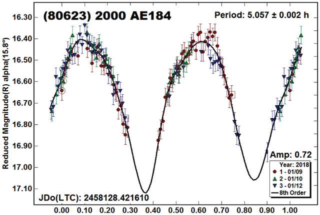
80623	2000 AE18 4	09–12	133	16.5,15.4	145	−7	5.057	0.002	0.66	0.03	FLOR	1.6	0.24
81788	2000 JQ81	11–12	132	13.0	145	−8	85	5	0.45	0.10	MB-O	2.6	0.258
107541	2001 DG7 0	09–11	187	16.7,16.1	144	−8	5.67	0.02	0.07	0.01	EUN	2.6	0.236
107541	2001 DG7 0						2.85	0.01	0.05	0.01
114095	2002 VY3 9	09–11	166	13.7,13.1	145	−8	6.88	0.02	0.21	0.02	MB-O	4.8	0.057
128071	2003 OS9	10–11	103	12.2,12.0	145	−8	17.92	0.05	0.33	0.02	MB-O	8.1	0.052
128843	2004 RH341	10–11	194	13.2,12.9	146	−8	10.87	0.03	0.33	0.02	MB-O	4.2	0.213
129437	1978 NG	09–11	143	11.6,11.1	147	−9	6.221	0.004	0.38	0.02	MB-O	3.3	0.301
132691	2002 NY32	09–12	132	12.9,12.2	147	−9	14.5	0.1	0.13	0.02	EUN	2.4	0.297
145425	2005 QP39	09–12	142	13.5,12.7	146	−8	200.	15.	0.6	0.1	MB-O	5.0	0.103
149646	2004 FX34	10–12	140	18.4,17.7	144	−7	3.930	0.004	0.17	0.02	FLOR	1.5	0.24
166342	2002 JV132	12–12	26	12.4	145	−8	3.7	0.3	0.23	0.02	MB-I	4.0	0.041
177012	2003 BU24	09–11	154	14.1,13.5	145	−9	10.58	0.02	0.45	0.02	MB-O	3.9	0.057
181249	Tkachenko	09–11	116	12.2,11.7	146	−9	2.19	0.02	0.06	0.03	MB-O	3.5	0.089
181931	1999 TJ138	09–12	136	12.3,11.6	147	.9	3.662	0.002	0.24	0.02	MB-O	5.1	0.074
188451	2004 HR5 9	10–12	151	16.5,15.9	145	−8	-	-	-	-	V	1.6	0.20
218827	2006 TJ68	09–12	124	18.2,17.0	143	−7	7.19	0.02	0.13	0.02	FLOR	1.3	0.24
218827	2006 TJ68	09–12					3.60	0.01	0.15	0.02
237192	2008 UA242	12–12	43	14.2	145	−8	4.2	0.2	0.48	0.03	EUN	1.4	0.21
259650	2003 WH103	12–12	43	16.6	145	−7	3.6	0.2	0.13	0.01	FLOR	1.3	0.24
283691	2002 RH80	10–11	119	14.5,14.2	145	−9	7.98	0.02	0.28	0.02	MB-O	3.3	0.057
300697	2007 VE63	09–11	98	15.0,14.4	145	−7	7.51	0.02	0.21	0.02	MB-O	3.7	0.057
310876	2003 KV33	09–11	79	13.7,13.2	145	−8	2.07	0.01	0.16	0.02	MB-O	3.5	0.057
319017	2005 UU511	09–12	132	13.6,12.8	145	−9	2.45	0.01	0.05	0.01	MB-O	3.9	0.057
321706	2010 GA3	09–11	128	7.6,7.3	149	−8	6.26	0.01	0.17	0.02	TR-J	16.1	0.057
321706	2010 GA3						3.13	0.01	0.15	0.02
322436	2011 SP247	12–12	38	12.1	146	−8	6.2	0.1	0.21	0.02	MB-O	3.9	0.057
322436	2011 SP247						3.1	0.1	0.21	0.02	MB-O
342436	2008 UT93	11–12	75	15.8,15.4	144	−9	6.63	0.05	0.22	0.02	MB-M	2.4	0.10
381809	2009 UC135	09–12	121	17.4,16.3	143	−8	2.56	0.01	0.11	0.02	MB-I	1.5	0.109
387906	2004 XQ	10–11	123	14.5,14.2	145	−8	4.945	0.003	0.38	0.02	EUN	2.2	0.194
395907	2013 AC78	09–12	96	14.8,14.0	145	−9	5.330	0.002	0.70	0.05	MB-O	3.1	0.057
396929	2005 FQ7	10–10	56	17.1	145	−7	4.03	0.01	0.16	0.02	EUN	1.3	0.21
399912	2005 XG7 5	09–09	15	13.9	145	−9	3.0	0.1	0.13	0.02	MB-O	4.6	0.057
420280	2011 OC2 6	11–11	34	19.1	143	−7	8.6	0.5	0.44	0.05	H	0.6	0.30
437408	2013 WQ8 3	10–12	99	18.0,17.6	143	−8	14.45	0.10	0.11	0.02	FLOR	0.9	0.24
438202	2005 UE129	12–12	33	17.9	143	−7	>14	-	>0.2	-	V	0.9	0.20
440931	2006 XK39	09–11	151	14.7,14.4	159	−8	3.33	0.01	0.08	0.02	MB-O	3.5	0.057
469419	2001 XA249	09–12	109	13.2,12.4	146	−7	29.6	0.5	0.30	0.03	MB-O	4.2	0.057
513494	2009 FC57	12–12	38	15.2	146	−8	7.5	1.0	>0.3		MB-O	2.5	0.057
513720	2012 TB4	11–11	44	16.1	143	−8	6.3	0.5	0.51	0.03	EUN	1.1	0.21
518966	2010 HL45	12–12	47	14.4	145	−8	-	-	-	-	MB-O	2.9	0.027
	2010 OE84	10–11	51	15.6,15.3	145	−7	8.81	0.04	0.63	0.03	MB-M	2.3	0.083
	2011 QO3	09–12	116	6.8,6.4	149	−9	5.67	0.01	0.34	0.04	TR-J	15.3	0.057
	2018 AL11	09–11	52	13.5,13.0	145	−8	2.891	0.006	0.18	0.02	MB-O	3.5	0.057

About the Lightcurve Plots and LCDB References

Only two objects had previous lightcurve entries in the asteroid lightcurve database (LCDB; Warner et al., 2009), which is available at http://www.minorplanet.info/lightcurvedatabase.html. Those previous results are referenced directly in the discussion for the asteroid in question.

The LCDB page allows direct queries of the LCDB that can be filtered a number of ways and the results saved to a text file. A set of text files of the main LCDB tables, including the references with bibcode, is also available for download. Readers are strongly encouraged to obtain, when possible, the original references listed in the LCDB for their work.

In the plots below, the “Reduced Magnitude” is Cousins R_c as indicated in the Y-axis title. These are values that have been converted from sky magnitudes to unity distance by applying −5*log (rΔ) to the measured sky magnitudes with r and Δ being, respectively, the Sun-asteroid and Earth-asteroid distances in AU. The magnitudes were normalized to the phase angle in the parentheses using G = 0.15, unless otherwise stated. The X-axis is the rotational phase ranging from −0.05 to 1.05.

If the plot includes an amplitude, e.g., “Amp: 0.65”, this is the amplitude of the Fourier model curve and not necessarily the adopted amplitude for the lightcurve.

Many of the lightcurves are presented without comment. Where required, a discussion of the results is included.

1992 Galvarino, 6594 Tasman.

Birlan et al. (1996) found a period of 7.004 hr for 1992 Galvarino. The period here is essentially identical. The LCDB had no lightcurve entries for 6594 Tasman.

15132 Steigmeyer.

There was only one night of extended observations. Based on the slope joining the two nights, the slope of the data on the extended night, and assuming the two sessions were each at an extrema, a period of about 115 hr is a plausible solution. If nothing else, this forewarns those making future observations that an extended campaign might be required.

(16364) 1979 MA5.

A half-period solution was used to help remove ambiguities for the full period. Given the 0.6 mag amplitude and low phase angle, a bimodal solution is all but guaranteed (Harris et al., 2014).

The three upcoming apparitions, 2019 April, 2020 July, and 2021October are V ≤ 18, or within reach of those with 0.5-m or larger telescopes.

24986 Yalefan.

There were no previously reported rotation periods in the LCDB. For backyard observers, the next good chance comes in 2023 September (V = 16.3).

40328 Dow.

No solution with a plausible fit of the Fourier curve could be found. The plot shows the raw data from three nights. The 2019 July apparition is at V = 16.8, making it a relatively easy target.

(44779) 1999 TM153.

The period spectrum shows several possible solutions. Two solutions are given on the presumption of a monomodal or bimodal lightcurve. A higher-modal lightcurve (longer period) would have produced even larger gaps, almost assuring a fit by exclusion. In this case, we have adopted the longer (“full”) period of 7.43 hr.

15132 Steigmeyer.

There was only one night of extended observations. Based on the slope joining the two nights, the slope of the data on the extended night, and assuming the two sessions were each at an extrema, a period of about 115 hr is a plausible solution. If nothing else, this forewarns those making future observations that an extended campaign might be required.

(16364) 1979 MA5.

A half-period solution was used to help remove ambiguities for the full period. Given the 0.6 mag amplitude and low phase angle, a bimodal solution is all but guaranteed (Harris et al., 2014).

The three upcoming apparitions, 2019 April, 2020 July, and 2021October are V ≤ 18, or within reach of those with 0.5-m or larger telescopes.

24986 Yalefan.

There were no previously reported rotation periods in the LCDB. For backyard observers, the next good chance comes in 2023 September (V = 16.3).

40328 Dow.

No solution with a plausible fit of the Fourier curve could be found. The plot shows the raw data from three nights. The 2019 July apparition is at V = 16.8, making it a relatively easy target.

(44779) 1999 TM153.

The period spectrum shows several possible solutions. Two solutions are given on the presumption of a monomodal or bimodal lightcurve. A higher-modal lightcurve (longer period) would have produced even larger gaps, almost assuring a fit by exclusion. In this case, we have adopted the longer (“full”) period of 7.43 hr.

(47048) 1998 WW18.

Using data from multiple sources, Durech et al. (2018) found a shape and spin axis model with a sidereal period of 12.82438 hr. The “Pref” and “Alt” lightcurves are based on no zero point adjustments to the original data.

It was possible to get an approximate match to the Durech et al. period (“Forced”) but only with zero point adjustments of 0.05–0.07 mag. Almost all other lightcurves required no more than a 0.02 mag adjustment to fine-tune the result, making the 12-hour solution dubious when based on our data alone.

The apparitions in 2019 May and 2020 September are V = 17.2. Those will be good opportunities to find a better solution for the rotation period.

(52441) 1994 RS1.

The period spectrum was very vague. Monomodal and bimodal solutions are given with the “full” period preferred because of the amplitude (Harris et al., 2014).

(62376) 2000 SU153.

The period is a best guess and could easily be wrong. It is presented to indicate that data are available.

(68414) 2001 QA219, (80234) 1999 VK195.

There were insufficient data for 2001 QA219 to show a definitive up or down trend let alone to find a period and so only the raw plot (mag vs. JD) is shown. It reaches V = 16.1 in 2019 August.

Despite the low amplitude, the solution for 1999 VK195 is considered nearly secure. Lightcurves using a half or double period, and others, were unrealistic and/or required excessive zero point adjustments.

(80623) 2000 AE184.

Neither the half- or full-period lightcurve was entirely covered by the data. The large amplitude at a relatively low phase angle assures a bimodal solution (Harris et al., 2014). The 2020 November apparition is V = 18.2 for those looking to get a complete lightcurve.

(81788) 2000 JQ81.

Using the slope of the data between the two nights, the slope of the data on January 12, and assuming a symmetrical bimodal lightcurve that takes about 0.25 rotation phase to go from one extrema to the next, produces a solution of about 85 hr. This result should not be used for statistical rotation studies.

The 2019 June apparition is V = 18.3, followed by 2020 October (V = 18.8) and 2023 March (V = 18.5). It will likely take a coordinated observing campaign with observers who are well-separated in longitude to find the rotation period.

(107541) 2001 DG70.

The low amplitude produced a highly-ambiguous solution set. We adopted periods that produce either a monomodal or bimodal lightcurve. By default, we adopted the “full” period of 5.67 hr for this work.

Until the apparition in 2031 March (V = 17.9), a 1–2 meter telescope will be required to get useful photometry.

(114095) 2002 VY39.

Despite the asymmetry of the lightcurve, this appeared to be the most likely solution. There are no apparitions V ≤ 18.8 through 2050.

(128071) 2003 OS9.

The amplitude almost assures a bimodal lightcurve (Harris et al., 2014). Based on this, the data fit well to a period of 17.92 hr using 2^nd order analysis. Higher orders produced unrealistic model curves. Apparitions V < 19 and away from low galactic latitudes are rare; the next one is 2041.

(128843) 2004 RH341.

The half-period lightcurve was used to find the preferred full period of 10.98 hr. The resulting Fourier curve had an excessively deep, artificial minimum between 0.7–1.0 rotation phase; this was removed for the final lightcurve plot.

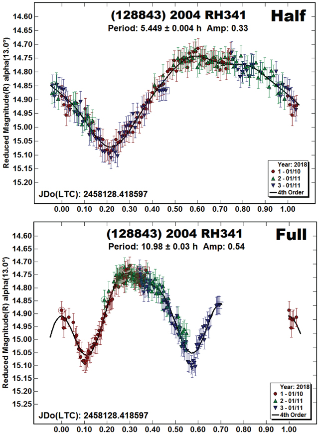
The asteroid will reach V = 18.7 in 2024 March, the next time it’s one that is also not close to the galactic plane.

(129437) 1978 NG, (132691) 2002 NY32.

The solution for 1978 NG is considered nearly secure, the main concern being the lack multiple coverage between 0.60 and 1.0 rotation phase.

For 2002 NY32, a half-period solution near 7.25 hr was affected by what would be the asymmetry of the full-period lightcurve at 14.5 hr. The result is good enough for statistical studies but needs confirmation. For those with 1–2 meter telescopes, the next chance comes in 2020 October (V = 18.8)

(145425) 2005 QP39.

The full period is based on the assumption of a symmetrical bimodal lightcurve. Doubling the half-period gives a result that is within 1-sigma of the full period error. All apparitions through 2050 are V ≥ 19.0.

(149646) 2004 FX34.

The period spectrum shows the “best” period as 5.9 hr. However, this gave an asymmetrical lightcurve with a large gap over about 0.2 rotation phase. This was taken to be a fit by exclusion and not the true period. Therefore, we adopted the next best, shorter period solution.

V = 18.9 is the brightest that 2005 OP39 will be through 2050; that is in 2020 November.

(166342) 2002 JV132, (177012) 2003 BU24.

The period for 2002 JV132 is likely wrong. The lightcurve is included to show that data are available. The 2019 apparition is at V = 18.0 in June, but at galactic latitudes near 0° (almost directly in front of the galactic center.

On the other hand, the solution of 10.58 hr for 2003 BU24 is very nearly secure, i.e., the period is almost certainly correct, but the shape of the lightcurve is not fully defined.

This asteroid barely reaches V = 19 through 2050. A 1–2 meter telescope will be needed to confirm these results.

181249 Tkachenko.

The lightcurve is presented to indicate that data were available and show their general quality. The period solution should not be used for statistical rotation period analysis. Large telescope owners (D > 1 m) might try to find a period in 2021 October when the asteroid reaches V = 19.3.

(181931) 1999 TJ138.

The amplitude, which nearly assures a bimodal solution (Harris et al., 2014), helped remove several longer periods with accompanying higher-modal lightcurves

(188451) 2004 HR59.

No solution could be found. The raw plot is used to show the quality and any trends in the data. All the brighter apparitions take place in the southern celestial hemisphere. The two closest ones with V ≤ 19.0 take place in 2022 April and 2026 June.

The 2019 apparition reaches brightest, V = 19.3, on Aug 3.

(218827) 2006 TJ68.

Neither the half-period (monomodal) nor the full-period (bimodal) solution can be formally excluded; the preferred solution is the full-period of 7.19 hr.

It might be possible to resolve the ambiguity in 2020 November when 2006 TJ68 reaches V = 18.5.

(237192) 2008 UA242.

The raw and half-period plots support our adopted period of 4.8 hr with a bimodal lightcurve. However, this needs confirmation. Unfortunately, the next time 2008 UA242 is V ≤ 19.0 is 2037 November. Until then, it hovers near V = 20 at brightest during an apparition.

(259650) 2003 WH103.

The period of 3.6 hr is a best fit of the data. The lightcurve amplitude is on the order of error bars and, with only one night of data, the solution should not be used for statistical studies. The next apparition that’s not too close to the galactic plane and might be within reach of 0.5–1.0 meter telescopes is 2023 September at V = 18.5.

(283691) 2002 RH80.

The period is almost exactly commensurate with an Earth-day. Other commensurate periods, e.g., 4, 6, 12 hr, were eliminated by using a half-period solution and considering that the amplitude approaching 0.30 mag made a bimodal lightcurve likely. The 2025 September apparition is the next one with reasonable chances of success with a 1–2 meter telescope (V = 19.4).

(300697) 2007 VE63, (310876) 2003 KV33.

There were no rotational period entries in the LCDB for either asteroid. Of the two, the solution for 2003 KV is considered secure. The solution for 2007 VE63 needs confirmation. That will require a 1–2 meter telescope since the asteroid is V ≥ 19.4 through 2050.

(319017) 2005 UU511.

This is a weak solution that is very possibly wrong. The brightest 2005 UU511 gets through 2050 is V = 19.7. It and others V < 20 are in December at low galactic latitudes.

(321706) 2010 GA3.

The significant gap in the full-period solution might be considered a fit by exclusion. However, the two halves of the bimodal lightcurve are different enough that the 6.26 hr period cannot be formally excluded.

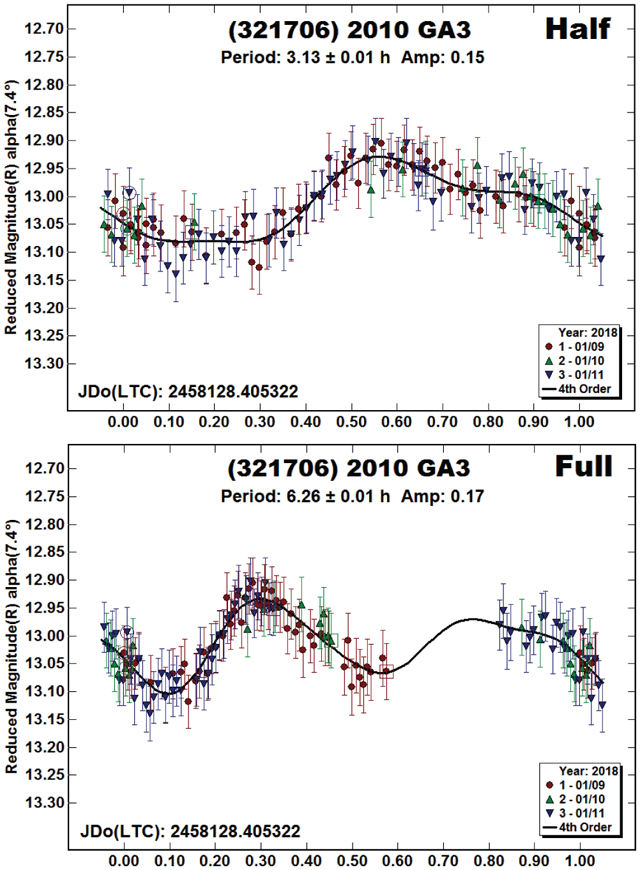
Looking ahead through 2050, the asteroid is between V = 19.4–19.9 at every apparition. The brightest one in the next ten years is 2023 August at V = 19.4.

(322436) 2011 SP247.

The half-period solution supports the adopted period of 6.2 hr. Because of the low amplitude, neither solution can be formally excluded (Harris et al., 2014).

Starting with 2020 August 22.3, 2011 SP247 reaches V = 19.5 and every five years plus ~ 2.2 days after. In 2050, the date of brightest will have moved into September (4.3). The declination on the date of brightest is about −3° each time.

(342436) 2008 UT93, (381809) 2009 UC135, (387906) 2004 XQ.

The period of 6.63 hr for 2008 UT93 represents the best fit among several possibilities. The asteroid will be V = 19.2 in 2022 January, the next “best” apparition.

Trimodal lightcurves are not uncommon at low amplitudes (Harris et al., 2014) and so, for 2009 UC135, the period is supported by the asymmetry of the lightcurve. A forced solution with a (nearly) bimodal solution was unsatisfactory. Finding the true period will be difficult since 2009 UC135 is rarely brighter than V = 20. The next opportunity is 2020 October at V = 19.7.

The solution for 2004 XQ is considered secure: there is complete coverage and the amplitude assures a bimodal lightcurve.

(395907) 2013 AC78.

A period of 5.33 hr produced the most symmetrical lightcurve when assuming a total rise or fall from one extrema to the next of 0.25 rotation phase. The period represents 4.5 rotations per Earth day. Without a 2-m telescope, there probably won’t be another lightcurve through at least 2050.

(396929) 2005 FQ7.

The period spectrum showed numerous nearly-equal minimums. A bimodal lightcurve had too large of gaps to make it preferable to the monomodal lightcurve of 4.03 hr. It’s not until 2027 March that 2005 FQ7 reaches V = 19.2. Until then it stays at V ≥ 20.0.

(399912) 2005 XG75.

The lightcurve is shown to indicate that data were available and their general quality. The solution is very possibly wrong since it presumes a low-amplitude bimodal lightcurve. 2024 March (V = 19.4) is the next “good” apparition.

(420280) 2011 OC26.

The half-period lightcurve is too asymmetrical to presume a secure solution for the adopted full-period solution of 8.6 hr. However, the monomodal lightcurve helped establish a reasonable estimate of the actual lightcurve amplitude. The next noteworthy apparition is 2024 August (V = 18.6).

(437408) 2013 WQ83, (438202) 2005 UE129, (440931) 2006 XK39.

The solution for 2013 WQ83 could easily be a fit by exclusion. However, no other period gave a more plausible result. The data set for 2005 UE129 was too limited to say more than the period is likely >10 hr.

The solution for 2006 XK39 is considered secure. The half-period of 1.66 hr can be safely excluded given the estimated diameter of 4.5 km. The combination would place it too far above the so-called “spin barrier” of about 2.2 hr to be plausible.

For 2013 WQ83, 2020 October (V = 19.6) is the next apparition with some hope of finding the period, but only with a 1–2 meter telescope. The prospects for 2005 UE129 are even less promising: V = 19.8 is the best it can do, the next time is 2032 December.

(469419) 2001 XA249, (513494) 2009 FC57, (513720) 2012 TB4, (518966) 2010 HL45.

For the first three asteroids, the adopted period is a best estimate based on the slopes of data for the individual nights and a presumed amplitude of about 0.3 mag or larger. For 2010 HL45, no solution could be found and so only a plot of the raw data (mag vs. JD) is given.

2009 FC57 reaches V = 19.2 in 2023 April. The others rarely reach V ≤ 20.0 through 2050.

2010 OE84.

The period spectrum gave limited guidance when trying to establish the true period. All of the solutions between 6 and 15 hr produced lightcurves that were less than fully convincing. The next good apparition is 2031 February at V = 19.4.

2011 QO3, 2018 AL11.

The solution for 2011 QO3 is based on using the full data set. If the data from January 9 are excluded, shorter periods between 2–4 hr become possible, but without nearly as good a fit as with the full data set. In 2022 July, 2011 QO3 brightens to V = 19.0.

The solution for 2018 AL11 is good enough for the period to be used in statistical studies, but it should not be considered definitive. The few apparitions when V < 20 through 2050 are at low galactic latitudes.

Original Data

The data for the 53 asteroids in this paper have been uploaded to the ALCDEF site (http://alcdef.com).

References

- Berthier J, Vachier F, Thuillot W, Fernique P, Ochsenbein F, Genova F, Lainey V, Arlot J-E (2006). “SkyBoT, a new VO service to identify Solar System Objects.” in Astronomical Data Analysis Software and Systems XV. ASP Conference Series 351, 367. Astronomical Society of the Pacific. San Francisco. [Google Scholar]
- Birlan M, Barucci MA, Angeli CA, Doressoundiram A, De Sanctis MC (1996). “Rotational properties of asteroids: CCD observations of nine small asteroids.” Planet. Space Sci 44, 555–558. [Google Scholar]
- Durech J, Hanus J, Ali-Lagoa V (2018). “Asteroid models reconstructed from the Lowell Photometric Database and WISE data.” Astron. Astrophys 617, A57. [Google Scholar]
- Erasmus N, McNeill A, Mommert M, Trilling DE. Sicakfoose AA, van Gend C. (2018). “Taxonomy and Light-curve Data of 1000 Serendipitously Observed Main-belt Asteroids.” Ap. J. Suppl 237, A19. [Google Scholar]
- Harris AW, Young JW, Scaltriti F, Zappala V (1984). “Lightcurves and phase relations of the asteroids 82 Alkmene and 444 Gyptis.” Icarus 57, 251–258. [Google Scholar]
- Harris AW, Young JW, Bowell E, Martin LJ, Millis RL, Poutanen M, Scaltriti F, Zappala V, Schober HJ, Debehogne H, Zeigler KW (1989). “Photoelectric Observations of Asteroids 3, 24, 60, 261, and 863.” Icarus 77, 171–186. [Google Scholar]
- Harris AW, Pravec P, Galad A, Skiff BA, Warner BD, Vilagi J, Gajdos S, Carbognani A, Hornoch K, Kusnirak P, Cooney WR, Gross J, Terrell D, Higgins D, Bowell E, Koehn BW (2014). “On the maximum amplitude of harmonics on an asteroid lightcurve.” Icarus 235, 55–59. [Google Scholar]
- Kim S-L, Lee C-U, Park B-G, Kim D-J, Cha S-M, Lee Y, Han C, Chun MY, Yuk I (2016). “KMTNET: A Network of 1.6 m Wide-Field Optical Telescopes Installed at Three Southern Observatories.” J. Korean Ast. Soc 49, 37–44. [Google Scholar]
- Mainzer AK, Bauer JM, Cutri RM, Grav T, Kramer EA, Masiero JR, Nugent CR, Sonnett SM, Stevenson RA, Wright EL (2016). “NEOWISE Diameters and Albedos V1.0.” NASA Planetary Data System. EAR-A-COMPIL-5-NEOWISEDIAM-V1.0 [Google Scholar]
- Mommert M (2017). “PHOTOMETRYPIPELINE: An automated pipeline for calibrated photometry.” Astronomy and Computing 18, 47–53. [Google Scholar]
- Pravec P, Hergenrother C, Whiteley R, Sarounova L, Kusnirak P (2000). “Fast Rotating Asteroids 1999 TY2, 1999 SF10, and 1998 WB2.” Icarus 147, 477–486. [Google Scholar]
- Warner BD, Harris AW, Pravec P (2009). “The Asteroid Lightcurve Database.” Icarus 202, 134–146. Updated 2018 June. http://www.minorplanet.info/lightcurvedatabase.html [Google Scholar]