Abstract
Air travel facilitates the international spread of infectious disease. While global air travel data represent the volume of travel between airports, identifying which airport an infected individual might use, or where a disease might spread after an infected passenger deplanes, remains a largely unexplored area of research and public health practice. This gap can be addressed by estimating airport catchment areas. This research aims to determine how existing market area delineation techniques estimate airport catchments differently, and which techniques are best suited to anticipate where infectious diseases may spread. Multiple techniques were tested for airports in the Province of Ontario, Canada: circular buffers, drive-time buffers, Thiessen polygons, and the Huff model, with multiple variations tested for some techniques. The results were compared qualitatively and quantitatively based on spatial patterns as well as area and population of each catchment area. There were notable differences, specifically between deterministic and probabilistic approaches. Deterministic techniques may only be suitable if all airports in a study area are similar in terms of attractiveness. The probabilistic Huff model appeared to produce more realistic results because it accounted for variation in airport attractiveness. Additionally, the Huff model requires few inputs and therefore would be efficient to execute in situations where time, resources, and data are limited.
Keywords: Airport catchments, Huff model, Infectious disease, Public health, Retail geography
Research Background
Air travel is a key mechanism facilitating the international spread of infectious disease. The increasing volume and ease of air travel promotes the dispersal of pathogens and importation of infectious diseases worldwide. This poses a significant threat to environmental conservation and public health (Golnar et al. 2016; Hatcher et al. 2012; Kilpatrick et al. 2006; Tatem et al. 2006). Severe acute respiratory syndrome (SARS), West Nile virus and Zika virus are well-known examples of this phenomenon (Bird and McElroy 2016; Bogoch et al. 2016a, b; Fauci and Morens 2016; Golnar et al. 2016; Lounibos 2002; Powers 2015; The SARS Commission 2006). The majority of processes that aim to address infectious disease threats are reactive in nature (Kilpatrick et al. 2006). In response to events such as the outbreaks of SARS, West Nile and Zika, researchers have increasingly studied the global movement of humans to predict and possibly prevent the emergence of infectious disease. However, this has proven to be notoriously difficult, and many approaches involve numerous assumptions and analyses based on incomplete data (Kilpatrick et al. 2006). Despite these inherent challenges, researchers continue to find new ways to provide necessary support to decision-makers (Golnar et al. 2016).
Multiple studies have identified human air travel as one of the most important pathways for the importation of infectious disease to new areas (Golnar et al. 2016; Kilpatrick et al. 2006). Data on passenger and flight volumes have been used to model international connections and anticipate where infectious diseases might be imported. For example, Bogoch et al. (2016a) analyzed air travel volumes for travelers departing Brazil, to anticipate the international spread of Zika virus during the 2016 outbreak. Such analyses aim to help health care workers anticipate whether they may see travel-related infectious disease cases, and support public health officials in guiding resource distribution (e.g. for screening or communication campaigns) to locations at risk for local transmission if a case was imported. In fact, Zika virus was presumably imported to Miami from Brazil via air travel, and local transmission was initiated due to the presence of Aedes mosquitos and suitable environmental conditions (Bogoch et al. 2016a, b; Centers for Disease Control and Prevention, 2017).
The processes of infectious disease importation and spread are complex, but simplified modelling efforts can be effective (Golnar et al. 2016). While analysis using global air travel data indicates volume of travel between airports, identifying which airport an infected individual might use, or where a disease might spread after an infected passenger deplanes, remains a largely unexplored area of research. This gap can be addressed by estimating the area from which an airport attracts its passengers, referred to as its catchment area (Lin et al. 2016). In the absence of observed data, airport catchment areas can be estimated through a variety of models. While many catchment area techniques were developed for trade area analysis in retail geography (Boots 1980; Huff 2003; Huff and Black 1997; Reilly 1931), they have also been applied to model service areas for transportation (Debrezion et al. 2009; Lin et al. 2016; Wittman 2014). Existing methods can be classified into three main categories: deterministic, probabilistic, and customer profiling (Hernandez et al. 2004). Only deterministic and probabilistic methods are relevant to this study, since data representing spatial concentrations of airport users, which would be necessary for customer profiling, are lacking.
Deterministic approaches make a clear-cut assumption about the spatial dimension of the trade area (Hernandez et al. 2004). Trade areas are polygons that have definite boundaries, and assume that all customers come from the defined catchment (Hernandez et al. 2004). Proximity-only models are included in the deterministic category and include circular buffers or drive-time buffers along a road network (Hernandez et al. 2004; Lin et al. 2016). Another deterministic technique calculates Thiessen polygons (also known as Voronoi polygons) around sites (Boots and South 1997; Hernandez et al. 2004). Here, every customer is assigned to the closest site based on Euclidean distance. Customers are assigned to only one site, and the mid-points between sites form the trade area boundaries. The Thiessen polygon method has been adapted to incorporate weights based on store/site attractiveness (Boots 1980; Hernandez et al. 2004). While deterministic methods such as circular buffers have been used to estimate airport catchment areas for the purpose of anticipating spread of infectious disease (Brent et al. 2018), they may over-simplify the problem (Cervero et al. 1995; Debrezion et al. 2009; Lin et al. 2016; Sanko and Shoji 2009).
In contrast to deterministic approaches, probabilistic approaches do not assume that customers always choose the closest option, and therefore assign customer groups (households, census tracts, neighbourhoods) partially to the alternative sites (Hernandez et al. 2004). A widely-used probabilistic model is the Huff model (Huff 2003), which defines catchment or trade areas as series of zonal probability contours (Huff 1963). The Huff model is popular in retail geography because it is relatively straightforward to apply, conceptually appealing, and applicable to a wide range of problems (Huff 2003; Huff and Black 1997).
The Huff model results represent the probability of the population at each origin location to patronize each alternative service location. The two basic parameters of the model are attraction and distance, both of which have explicit behavioural bases (Huff and Black 1997). The attraction parameter represents the “impact of store size on consumer patronage for a given product when distance is held constant” (Huff and Black 1997). For certain products or services, size (or other associated attractiveness measure) is more important to consumers, and therefore would more greatly impact their choice alternative. The distance decay parameter represents the consumer’s willingness to travel for different types of products (Huff 1963). The choice set is another critical element of the Huff model. In a choice situation, there exists a universal set of alternative sites from which a consumer selects a subset based on their individual preferences. For example, some choice alternatives may be beyond a maximum distance the consumer is willing to travel (Huff and Black 1997). Specifying an accurate choice set is essential to minimizing prediction errors (Huff and Black 1997).
When selecting a method to estimate airport catchment areas, it is important to consider existing knowledge of how airports are used. For example, Debrezion et al. (2009) found that less than half of passengers at a Dutch railway survey chose their nearest train station (Lin et al. 2016). Leon (2011) found that airline travellers in North Dakota will not use the local airport but instead use the competing major hub airport located 250 miles away. There is general consensus that consumers are willing to travel further to reach a more desirable location, but it is difficult to determine the maximum distance they would be willing to travel especially considering this distance likely changes between regions (Leon 2011; Lin et al. 2016). These examples suggest that for the application of delineating catchment areas for transportation, deterministic proximity-only models may be too coarse (Debrezion et al. 2009; Leon 2011; Lin et al. 2016; Wittman 2014), although circular buffers have been used frequently to define airport catchment areas (Bilotkach et al. 2012; McLay and Reynolds-Feighan 2006; Wang 2000; Wittman 2014). Lin et al. (2016) suggest that gravity models (such as the Huff model) may be a more appropriate approach than proximity-only approaches, since they incorporate not only distance but also attraction. The main considerations of the Huff model align with what studies have shown to be the greatest determinants of airport choice (Başar and Bhat 2004; Hess and Polak 2005; Ishii et al. 2009; Leon 2011; Suzuki 2007).
While some localized analyses have been conducted to model airport catchment areas (Augustyniak and Olipra 2014; Lieshout 2012), their techniques would be complex to apply at a national, or global scale. For example, if a drive-time distance or cut-off were incorporated in a model, it might be unrealistic to apply a single appropriate distance to the entire study area, where characteristics of the population and environment likely differ widely (Lin et al. 2016; Upchurch et al. 2004).
To support rapid response to infectious disease outbreaks, we explore the differences in how the multiple available methods estimate airport catchment areas. This research aims to answer two questions: How do various market area delineation techniques estimate airport catchments differently? And, which techniques are best suited to anticipate where infectious diseases may spread internationally? Airports in the Province of Ontario, Canada, served as a test case for which to compare results between techniques.
Data and Methods
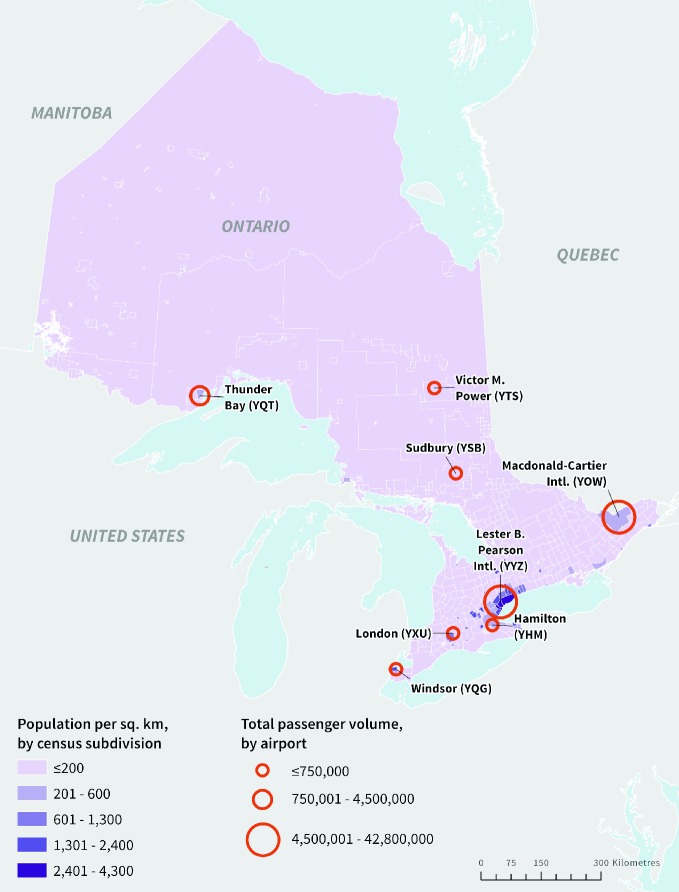
The case study of Ontario, Canada, was selected because of the province’s large territory and high population, and the relevant context of the outbreak of severe acute respiratory syndrome (SARS) in Toronto, Ontario, in 2003. Ontario is the second-largest province in Canada and home to over 13.5 million people (Government of Ontario 2018). The highest population densities are clustered around Toronto with smaller clusters of moderately-high population density near London, Hamilton, and Ottawa (Fig. 1). Ontario’s 77 airports are also concentrated in the south. Figure 1 shows the eight major airports that had 2016 passenger volumes reported by Statistics Canada.
Fig. 1.
Population density and locations of Ontario’s major airports by 2016 passenger volume (Statistics Canada 2016a)
Ontario’s high proportion of foreign-born population (29%) also makes the province relevant to this study (Ontario Ministry of Finance 2017). This high proportion is indicative of a high volume of transnational migrants, and increased frequency of cross-border travel for personal, education, and business purposes (Levitt and Jaworsky 2007). This phenomenon adds to the magnitude of international air travel to and from Ontario. The concern of importation of infectious disease via air travel is especially relevant to Toronto, in which immigrants make up close to one half of the city’s population. In 2003, Toronto experienced the largest outbreak of SARS outside of Asia (Bell 2004; Muller et al. 2006; Summers 2013). Bell (2004) noted “limiting the spread of infection by domestic and international travel” as one of the interventions that aided in containing this outbreak in some parts of the world. The importation of SARS to Toronto via international travel is an example of where interventions failed and had a devastating impact on both human health and the economy (The SARS Commission 2006).
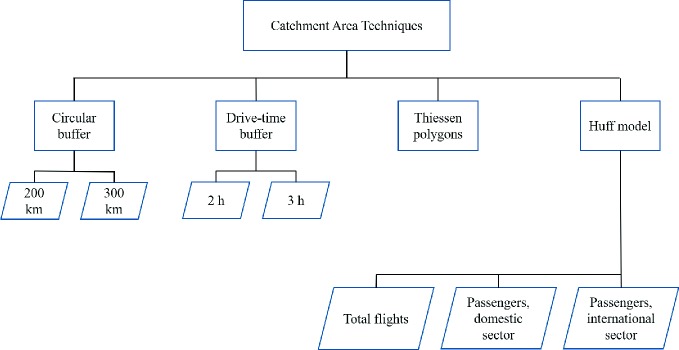
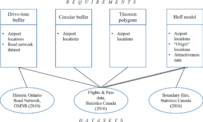
The catchment area delineation techniques applied to Ontario’s airports included three deterministic techniques (circular buffers, drive-time buffers, and Thiessen polygons) and one probabilistic technique (Huff model) (Fig. 2), with some variations based on parameter inputs. Each technique had unique data requirements (Fig. 3). Results from each technique were compared and evaluated based on the applicability to analyzing the potential for international spread of infectious disease. We assume that these methods are more representative of Ontario residents than tourists or visitors, who might take longer routes to reach various tourist attractions.
Fig. 2.
Catchment area delineation techniques applied to Ontario airports, with input specifications for circular buffer radius, drive-time extent, and the Huff model’s airport attractiveness metric
Fig. 3.
Data requirements and sources by catchment area delineation technique (double line indicates data source was used to fulfill two data requirements)
Data on air passenger traffic and flights for Ontario airports were obtained from Statistics Canada (2016a). Only eight of 77 airports had associated passenger traffic and flights data, as detailed in Table 1.
Table 1.
Airport passenger and flight volumes for 2016, where ‘−1’ indicates data were unavailable or suppressed (Statistics Canada 2016a)
| Name | Code | Pass. enplaned | Pass. deplaned | Total pass. | Domestic sector | Transborder sector | Intl. sector | Pass. flights |
|---|---|---|---|---|---|---|---|---|
| Toronto/Lester B Pearson | YYZ | 21,347,368 | 21,451,589 | 42,798,957 | 16,741,872 | 11,572,354 | 14,484,731 | 410,316 |
| Ottawa/Macdonald-Cartier Intl. | YOW | 2,303,278 | 2,304,815 | 4,608,093 | 3,607,040 | 611,089 | 389,964 | 72,787 |
| Thunder Bay | YQT | 377,176 | 376,445 | 753,621 | −1 | −1 | −1 | 27,463 |
| London | YXU | 257,516 | 250,689 | 508,205 | 467,075 | 17,758 | 23,372 | 10,277 |
| Timmins | YTS | 104,299 | 103,555 | 207,854 | 207,854 | 0 | 0 | 9475 |
| Sudbury | YSB | 113,888 | 113,315 | 227,203 | −1 | −1 | 0 | 8952 |
| Windsor | YQG | 160,068 | 159,254 | 319,322 | −1 | −1 | −1 | 6970 |
| Hamilton | YHM | 160,255 | 159,009 | 319,264 | 263,802 | −1 | −1 | 3816 |
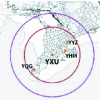
To estimate catchment areas using circular buffers the only necessary input was the spatial locations of the airports. Buffers were produced based on two distances: 200 and 300 km. Brent et al. (2018) applied a 200 km buffer to airports in their analysis of potential international spread of Yellow Fever globally. They used flight itinerary data of travelers who departed yellow fever-endemic areas. 200 km served as the lowest buffer distance. While visualized as full circles on the resulting map, the area and population associated with each buffer was calculated based only on the portion that intersected the Ontario boundary (including smaller inland water bodies but excluding the Great Lakes and Hudson’s Bay).
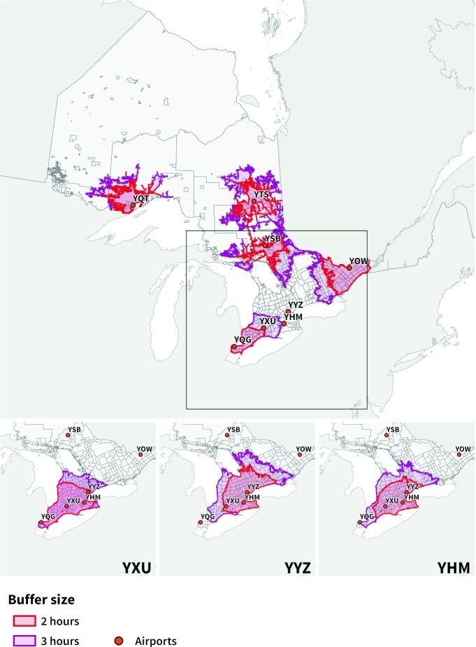
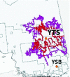
The drive-time buffers approach required an additional dataset representing the road network. A road network dataset was created for Ontario using a road network file from the Ontario Ministry of Natural Resources (2010). Since this road network covered Ontario only, resulting buffers were automatically restricted to provincial land. Buffers were produced based on two drive-time cut-offs: two and three hours. A maximum driving-distance to reach an airport in Ontario could not be referenced from existing literature. Thus, a 2-h cut-off was selected because preliminary exploration revealed that it was generally comparable in extent to the 200 km buffer for YYZ—the airport with the highest passenger volume (Table 1). A 3-h cut-off was also applied to include a larger drive-time cut-off for comparison.
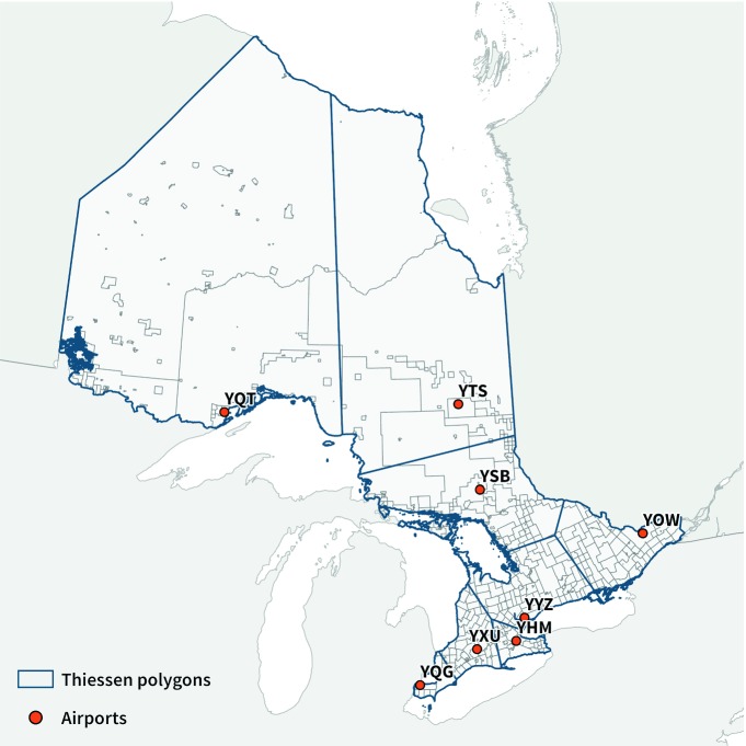
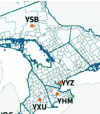
Like the circular buffer technique, Thiessen polygons required the single input of airport locations. Thiessen polygons form a tessellation that exhaustively fills the study area and do not overlap. Locations that are equally close to more than one airport collectively form the boundaries of the Thiessen polygons (Yamada 2016). In this study, each Thiessen polygon represented the catchment area of the respective airport.
The Huff model was the only probabilistic technique that was tested. It estimates catchment areas using both distance to and attractiveness of each airport, while also incorporating distance to and attractiveness of all other airports. The Huff model is described by:
 |
where Pij is the probability of an individual located at i choosing airport j, Sj is a measure of attractiveness for j, Dij is the distance from i to j, α is the attractiveness exponent and β is the distance decay exponent.
Probabilities were calculated for census subdivisions, which correspond to the municipalities (Statistics Canada 2016b), the level at which many public health programs and procedures are operationalized. To represent airport attractiveness, we tested multiple variables including total flights, total domestic passengers, and total international passengers. These data were obtained from the same Statistics Canada dataset that included airport locations. Parameterization of the Huff model was based on findings from a related study by one of the authors. On this basis, a value of 2 was applied as the distance decay exponent (beta), while no attractiveness exponent was applied (i.e., alpha = 1).
For all spatial analysis, modeling, and mapping, an open-source software package, QGIS, was used in conjunction with the “Location Analytics” toolset, which is under development (https://github.com/ryersongeo/qgis_location_analytics).
The results were visually compared within and between catchment area delineation techniques. Results were also quantitatively compared based on total area and population within each catchment area. For the Huff model, a probability threshold had to be defined to indicate which census subdivisions should be included in the area calculation. A minimum probability of 20% was selected to define the boundary of each catchment area. This threshold is similar to thresholds used to define market areas in the retail sector (Dolega et al. 2016). Population within each catchment area was calculated using population totals by census subdivision for 2016, obtained from Statistics Canada (2016c). For circular buffers, drive-time buffers, and Thiessen polygons, the total population within the catchment area was summed. If a subdivision was split by the catchment area boundary, the population of that subdivision was split proportionally based on area. For Huff model results, the population of each subdivision in the catchment area was multiplied by the probability of using each airport. The relationship between area and population for estimated catchment areas based on each technique was analyzed as an indicator of the spatial patterns of the risk of disease spread.
Analysis and Results
As expected based on the inherent characteristics of each technique, the estimated catchment areas notably differed. Results of each technique are shown in Figs. 4, 6, 8, 10, 11 and 12, which reveal qualitative differences in the shape and extent of catchment areas. Quantitative differences in the estimated area and population associated with each catchment are shown in Table 2.
Fig. 4.
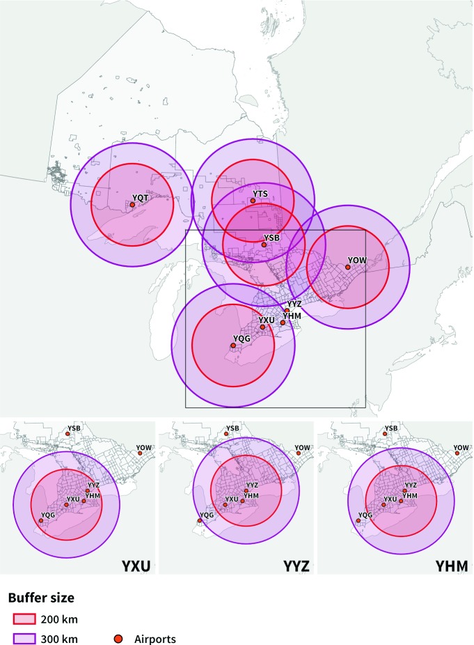
Circular buffers for major Ontario airports overlaid on census subdivision boundaries. Insets provided for the London, Toronto, and Hamilton airports in Southern Ontario
Fig. 6.
Drive-time buffers for major Ontario airports overlaid on census subdivision boundaries
Fig. 8.
Thiessen polygons for major Ontario airports overlaid on census subdivision boundaries
Fig. 10.
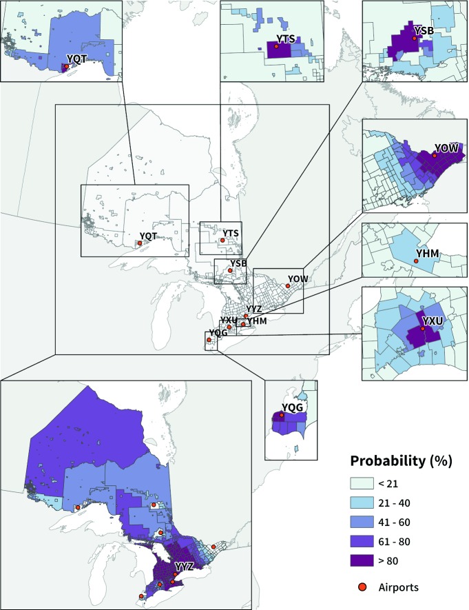
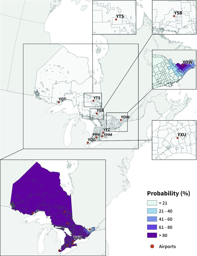
Huff model results for airports with greater than zero total enplanements or deplanements, with airport attractiveness represented by total passenger flights, reported by census subdivision
Fig. 11.
Huff model results for airports with greater than zero total enplanements or deplanements, with airport attractiveness represented by total domestic passengers, reported by census subdivision (airports not appearing in an inset map had suppressed or unavailable data)
Fig. 12.
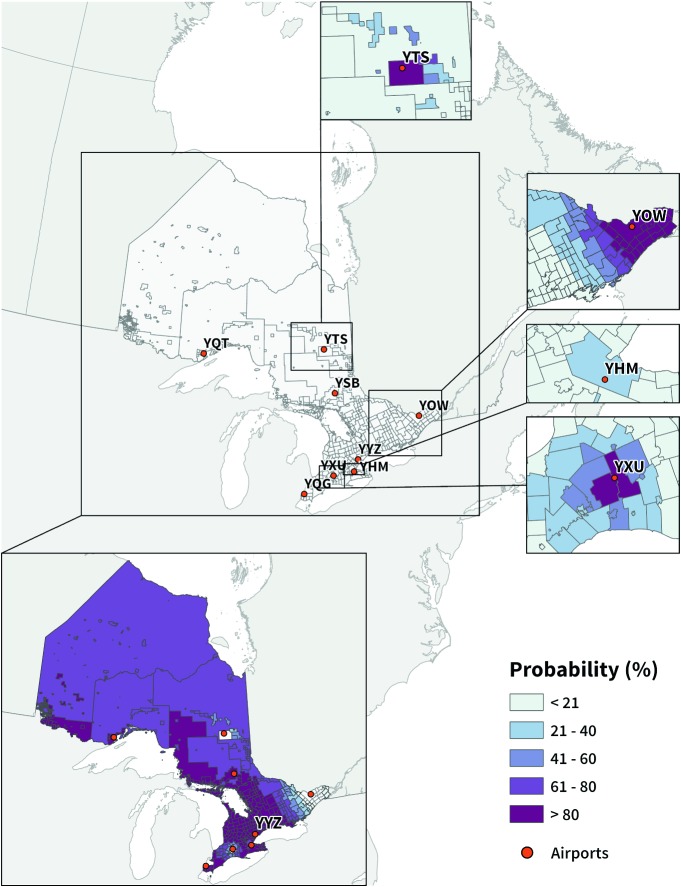
Huff model results for airports with greater than zero total enplanements or deplanements, with airport attractiveness represented by total international passengers, reported by census subdivision (airports not appearing in an inset map had suppressed or unavailable data)
Table 2.
Area (km2) and population for airport catchment areas as defined by different market area delineation methods
| Airport code | Circular buffers | |||
|---|---|---|---|---|
| 200 km | 300 km | |||
| Area | Population | Area | Population | |
| YYZ | 68,716 | 10,414,146 | 118,971 | 11,054,816 |
| YOW | 40,899 | 1,752,100 | 69,416 | 2,441,445 |
| YQT | 61,441 | 135,615 | 139,409 | 166,984 |
| YXU | 48,540 | 9,945,855 | 70,582 | 10,885,048 |
| YQG | 16,654 | 1,298,391 | 38,038 | 3,998,808 |
| YHM | 56,291 | 10,295,559 | 93,135 | 11,183,121 |
| YSB | 92,110 | 414,373 | 180,120 | 1,467,060 |
| YTS | 112,561 | 125,490 | 218,602 | 397,199 |
| Airport code | Drive-time buffers | Thiessen polygons | ||||
|---|---|---|---|---|---|---|
| 2 h | 3 h | |||||
| Area | Population | Area | Population | Area | Population | |
| YYZ | 39,248 | 9,663,296 | 72,801 | 10,573,212 | 40,378 | 7,366,464 |
| YOW | 20,304 | 1,415,375 | 34,790 | 1,669,496 | 40,487 | 1,707,563 |
| YQT | 10,962 | 112,798 | 21,605 | 116,650 | 497,319 | 227,353 |
| YXU | 33,978 | 5,818,639 | 49,786 | 10,210,489 | 19,072 | 982,067 |
| YQG | 9116 | 905,679 | 20,492 | 1,999,344 | 5161 | 549,935 |
| YHM | 32,642 | 9,309,201 | 59,500 | 10,385,373 | 8072 | 2,050,521 |
| YSB | 7805 | 118,815 | 24,820 | 234,147 | 80,232 | 452,685 |
| YTS | 12,394 | 39,614 | 29,551 | 82,002 | 293,508 | 111,906 |
| Airport code | Huff model | |||||
|---|---|---|---|---|---|---|
| Flights | Passengers, domestic sector | Passengers, intl. sector | ||||
| Area | Population | Area | Population | Area | Population | |
| YYZ | 961,118 | 10,285,369 | 968,352 | 10,812,078 | 981,143 | 12,146,910 |
| YOW | 35,000 | 1,366,554 | 44,206 | 1,397,449 | 17,137 | 1,032,229 |
| YQT | 143,910 | 162,333 | N/A | N/A | N/A | N/A |
| YXU | 6457 | 394,297 | 7638 | 410,131 | 867 | 91,049 |
| YQG | 2046 | 349,831 | N/A | N/A | N/A | N/A |
| YHM | 1152 | 123,331 | 1183 | 180,212 | N/A | N/A |
| YSB | 12,628 | 146,714 | N/A | N/A | 0 | 0 |
| YTS | 9642 | 55,226 | 8945 | 49,541 | 0 | 0 |
Circular Buffers
Despite the drastic difference in the number of annual passengers and flights between airports, the catchment sizes based on the circular buffers approach are equal by definition. The full circular buffers (shown in Fig. 4) were 125,535 km2 for the 200 km buffer, and 282,453 km2 for the 300 km buffer. Catchment areas were not impacted by the presence of other proximate airports—though this could have been incorporated if buffers were truncated.
The area and population for the portions of each catchment that were within the study area are detailed in Table 2. YTS was the largest in area for both the 200 km and 300 km buffer sizes at 112,561 km2 and 218,602 km2, respectively. YYZ and YHM had the largest population sizes based on both the 200 and 300 km circular buffers.
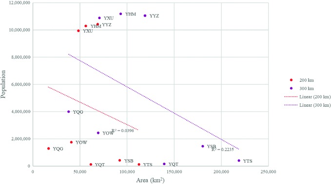
Figure 5 reveals that based on circular buffers, a larger catchment in terms of area was not necessarily associated with a larger population. While area was impacted by the proportion of the circular buffer that fell within the land boundaries of Ontario, the spatial distribution of population in the province meant that in many cases, circular buffers that had relatively small proportions of area falling within Ontario had the highest population sizes, and vice versa. For example, YYZ and YHM fell within the middle of all airports based on area but had the largest population. In contrast, YTS had the largest area but had one of the smallest populations. While the trend line in Fig. 5 shows that area was negatively associated with population, the relationship was weak and not statistically significant (r = −0.199, p = 0.637 for 200 km, and r = −0.437, p = 0.237 for 300 km).
Fig. 5.
Area and population for estimated airport catchment areas based on 200 and 300 km circular buffers
Drive-Time Buffers
Generally, the size of catchment areas based on 2-h and 3-h drive-time buffers was similar between airports (Fig. 6), but could be categorized into two main groups based on whether they were located in areas with relatively high or low population density. Figure 1 shows that YQT, YTS, and YSB are surrounded by census subdivisions with relatively low population density. The road network is also less dense here. For these airports, the extent of the catchment area formed a web-like shape around the major roads. Thus, the catchment areas covered less area. These airport catchments were less than 13,000 km2 based on a 2-h drive-time, and less than 30,000 km2 based on a 3-h drive-time (Table 2).
In contrast, Fig. 1 shows that YYZ, YOW, YXU, YQG, and YHM are surrounded by census subdivisions with relatively high population density. The road network is also denser here so the catchment areas formed a fuller polygon. The area of the catchments for four of these five airports (excluding YQG) was between 20,000 and 40,000 km2 based on a 2-h drive-time and between 34,000 and 73,000 km2 based on a 3-h drive-time (Table 2). For airports surrounded by higher population density, catchments based on drive-time were similar to the circular buffers in extent.
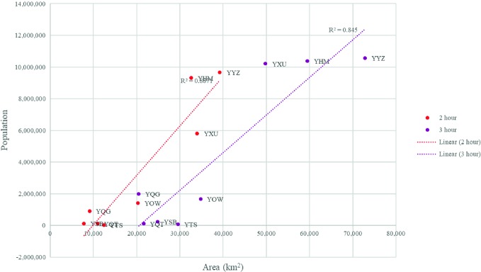
As shown in Fig. 7 and in contrast to circular buffers, based on the drive-time buffers approach there was a strong, positive correlation between area and population that was significant based on Pearson’s correlation coefficients (r = 0.942, p = 0.000 for 2-h, and r = 0.919, p = 0.001 for 3-h). For both buffer sizes, the airports with the largest catchments in terms of area also had the largest populations. As with circular buffers, YYZ and YHM had the largest catchment areas and associated populations.
Fig. 7.
Area and population for estimated airport catchment areas based on 2-h and 3-h drive-time buffers
Thiessen Polygons
In contrast to the two buffer approaches, there is great variation in the area of catchments based on Thiessen polygons (Fig. 8). Since there were more airports located in southern Ontario than in the rest of the province, catchment areas in southern Ontario were much smaller. Airports in less densely populated parts of Ontario, where fewer airport options existed, had much larger catchment areas. For example, Table 2 indicates that YQT located in northern Ontario had a catchment area of 497,319 km2 while YYZ located near Toronto only had an area of 40,378 km2. Both YQT and YTS had large catchment areas that extended to the northern boundary of the province.
Variation in population seemed to follow the opposite trend as variation in area. The airports in southern Ontario (plus YOW) tended to have larger population sizes associated with them even though the catchment areas were smaller. For example, Table 2 shows that a population of 227,353 fell within the catchment of YQT (northern Ontario), while a population of 7,366,464 fell within that of YYZ (southern Ontario). This follows the spatial pattern of population density in the province.
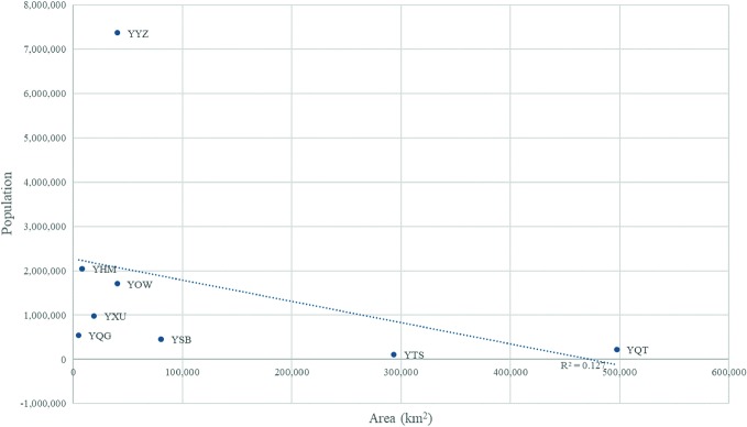
These findings are confirmed by Fig. 9, which shows that the airports with the larger catchments in terms of area did not necessarily have large populations. There was a negative correlation between area and population, though it was weak and not statistically significant (r = −0.356, p = 0.386). YYZ is most notable in Fig. 9, because it had a relatively small area but has a population much higher than any other airport.
Fig. 9.
Area and population for estimated airport catchment areas based on Thiessen polygons
Huff Model
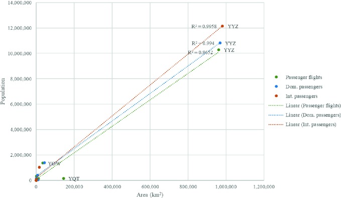
Estimated catchment areas based on the Huff model are shown in Figs. 10, 11 and 12, with airport attractiveness represented by total passenger flights, total domestic passengers, and total international passengers, respectively. Across all three variations of the Huff model, the most obvious pattern is that most census subdivisions were at least 40% likely to use YYZ over all other airports. Another notable characteristic of the Huff model results was that subdivisions located near one airport were less likely to use any other airport. While circular and drive-time buffers did not account for proximity to other airport options at all, Thiessen polygons arguably over-accounted for proximity to other airports by defining catchments based on only the midpoint between airport locations.
Between the Huff models based on total passenger flights, total domestic passengers, and total international passengers, very similar spatial patterns resulted. In all three cases, YYZ had the largest catchment, YOW had a moderately-large catchment, and all other airports were small or non-existent. A notable difference in results based on flight volume, domestic passenger volume, and international passenger volume can be seen in the results for YTS. For this airport, subdivisions within close proximity have greater than 40% probability to use the airport based on total flight volume and on domestic flight volume. However, without reported international passenger volume, this airport disappears from the corresponding Huff model. Results for YXU and YOW followed a similar pattern, since they had fewer international passengers as compared to domestic passengers or total flights. In contrast, there was a clear increase in probability to use YYZ when attractiveness was based on international travel volume, specifically into northern Ontario. YYZ’s catchment had an area of 981,143 km2 when airport attractiveness was based on international passenger volume, as compared to 968,352 km2 when it was based on domestic passenger volume (illustrated in Figs. 11 and 12).
Like Thiessen polygons, the Huff model produced large variation in the extent of each airport’s catchment area. While for Thiessen polygons this variation was the result of solely the distance between airports, variation produced by the Huff model was the result of both distance between airports and the attractiveness of each airport. Where YQT had the largest catchment area based on Thiessen polygons at 497,319 km2, YYZ had the largest catchment areas based on all three variations of the Huff model at approximately 970,000 km2 (Table 2).
This variation in area in turn impacted the catchment area populations with a strong, positive association between area and population based on the Huff model (Fig. 13). The Pearson’s correlation revealed that the relationship was significant for all three variations of results (r = 0.982, p = 0.000 for results based on passenger flights, r = 0.997, p = 0.000 for results based on domestic passengers, and r = 0.998, p = 0.000 for results based on international passengers. However, these statistics were likely impacted by YYZ being an outlier.
Fig. 13.
Area and population for estimated airport catchment areas based on the Huff model, using total passenger flights, domestic passengers, and international passengers to represent airport attractiveness
Discussion and Conclusion
This study illustrated that various market area delineation techniques produce notably different estimates of airport catchments. Differences existed in both the general shape and extent of the catchment areas as well as the land area and population associated with each. Moreover, area and population had varying relationships based on each technique. There were notable differences in the proportion of the study area belonging to each airport’s catchment based on the deterministic approaches (circular buffers, drive-time buffers, and Thiessen polygon) and the probabilistic approach (Huff model).
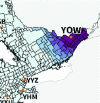
The application envisioned is the forecasting of the spread of infectious diseases. Such analyses often must be conducted rapidly, with limited data. Therefore, the trade-off between efficiency of execution and validity of results must be considered when evaluating each technique. Table 3 provides a summary of the evaluation of each technique based on this trade-off. While this study was conducted based on the test case of Ontario’s eight major airports, it is expected that results are generalizable to other areas.
Table 3.
Characteristics of catchment area techniques and results
| Circular buffers | Drive-time buffers | Thiessen polygons | Huff model | |
|---|---|---|---|---|
| Example |
|
|
|
|
| Efficiency to execute | Very efficient | Efficient | Very efficient | Efficient |
| Data requirements | Minimal | Minimal, but road network required | Minimal | Fairly minimal, origin and attractiveness data required |
| Input selection | Buffer distance fairly arbitrary | Buffer distance fairly arbitrary | Cannot adjust inputs to suit use case | Parameterization required |
| Result type | Binary | Binary | Binary | Probabilistic |
| Airport weighting | Weighted equally | Weighted equally | Weighted equally | Weighting by attractiveness |
| Coverage of study area | Partial coverage | Partial coverage | Full coverage | Full coverage |
| Other advantages | Results appear most realistic | |||
| Other limitations | Driving not always main method of transportation | Does not allow for catchment overlap | Can extent unrealistically far (without distance cut-off) |
Of the techniques tested, the circular buffers and Thiessen polygon approaches would be the most efficient to execute, since their only data inputs are the airport locations. However, selecting a radius for the circular buffer technique might be difficult due to limited recommendations for an appropriate distance. This parameter may also depend on the specific public health at hand. There were no inputs parameters required for the Thiessen polygon technique. While this makes it efficient to execute, it is impossible to tailor the method to the use case and study area of concern.
The drive-time buffer also required only the single parameter of a defined drive-time cut-off, but required the additional dataset for the road network. If an analyst had a defined study area in which they knew their analyses would be conducted, this network could be pre-processed. However, if this technique had to be executed for locations globally, it would likely require additional resources to prepare a road network dataset. Moreover, infectious disease events may occur in remote or rural areas, or in developing countries, for which road network data often do not exist or are not readily available. Furthermore, road transportation via vehicle is not always the main method of transportation in remote areas. For example, during the recent outbreak of Ebola in Bikoro, Democratic Republic of Congo, the primary transportation route to the nearest major population centres was not by road but via the Congo River (WHO 2018).
While the three deterministic methods can be efficient, the results for our study area did not appear to be realistic in the context of the differences in attractiveness between airports; there are few airports in Ontario with high flight and passenger volumes. The distance-only deterministic methods might be more appropriate in cases where airports are equally distributed across a study area and are similarly attractive. Alternatively, for circular and drive-time buffer methods multiple buffer sizes could be applied. For example, a larger buffer could be applied for international airports or those with higher passenger/flight volumes, and a smaller buffer could be applied for domestic airports or those with lower passenger/flight volumes. Overall, deterministic methods could likely provide a general estimate of airport catchment areas in time-limited situations, though results would come with numerous limitations.
The probabilistic Huff model required additional inputs but was still relatively efficient to execute. In contrast to the deterministic methods, the Huff model estimated the greatest variation between catchment areas of the different airports. While this study did not incorporate validation of results based on observed data, the Huff model results appear to be reasonable considering the passenger and flight volume associated with each airport. It would be expected that people travel from much further to reach YYZ due to its high volume of flights, and because they might not be able to travel to their intended destination from smaller airports in Ontario. However, the Huff model estimated that subdivisions even at the northern border of Ontario were most likely to use YYZ. This is unrealistic and could be addressed by defining a distance cut-off in the model to restrict the choice set to airports within a reasonable distance. Additionally, the Huff model, as it was implemented in this study, does not account for the potential of flight connections. For example, an individual could take a domestic flight from YTS to YYZ, and then fly to an international destination from YYZ. Such itineraries could be represented in the attractiveness variable if more detailed data were available.
The characteristics of results based on each technique must also be considered based on the situation in which this approach would be implemented. Specifically, it is important to consider whether full coverage of the study area is required, i.e. whether all locations in the study area must be assigned to at least one airport catchment area. This may be needed if the spread of a local outbreak through outbound passengers was to be forecast. Only the Thiessen polygon and Huff model techniques meet this requirement, while the buffering methods do not cover the entire study area. However, if considering an inbound infected individual, catchment area results would not necessarily need to cover the entire study area to estimate the area within which the individual would likely travel after deplaning.
Considering the context of SARS, all methods would have assigned the City of Toronto to YYZ. This was expected, due to Toronto’s close proximity to YYZ as well as the high volume of flights and passengers associated with YYZ. However, results based on each technique defined YYZ’s catchment area differently in extent—affecting the area that an infected traveler who deplaned at YYZ might travel to. The catchment area for YYZ, in this case, could be considered at risk for SARS spread. While the risk area based on Thiessen polygons was restricted to a small portion of southern Ontario, most of the province would have been included based on the Huff model. Resources might be focused on the defined risk area; therefore, it is important to select the most appropriate method, and apply appropriate data inputs, to best guide this distribution of resources. Considering YYZ’s high flight and passenger volume compared to the other airports, it may be possible that its true catchment area covers a large portion of the province, as estimated by the Huff model. In this case, it could be useful to incorporate the population distribution within the catchment area to help guide resource distribution, as is common in the field of retail geography to estimate the spatial distribution of potential customers.
The results of this study were impacted by limitations in data access and conceptualization of air travel. In the airport locations and associated passenger dataset obtained from Statistics Canada, some data were suppressed and at least one important airport location was not included for unknown reasons. In future research, Billy Bishop Airport (YTZ) in Toronto, which serves approximately 2.8 million travelers annually (PortsToronto 2018), should be included to better understand its impact on the catchment area of Pearson International Airport (YYZ). Second, the comparison between results based on domestic and international passengers did not include travel to the U.S., since that is included in the “transborder” variable. Additional analysis could be conducted to analyze results based on travel to the U.S. specifically, or the variable could be merged with international passengers. Third, the open-source Huff model tool did not have an option to apply a distance cut-off to represent a maximum distance that an individual would be willing to travel. Without the use of a distance cut-off, Toronto’s YYZ received high probability for individuals living in northern Ontario—in some cases over 1500 km away. The option to apply a distance cut-off would ensure a more realistic representation of travel to airports. Instead of travelling an unreasonably far distance, someone might choose to take a connecting flight from a local airport to a larger, more attractive airport from which to fly to their final destination. There was no obvious solution to including connecting flights in the modeling approaches, yet this would likely result in larger at-risk areas. Essentially, the catchment areas of larger airports would need to be extended to include the local catchments of smaller, connected airports, resulting in a network of airport catchment areas. Fourth, the methods did not consider airports outside of Ontario, such as US airports in Buffalo and Detroit just outside the Canadian border, which would likely reduce the estimated catchment sizes of some southern Ontario airports. Addressing this limitation would require expanding the study area to include parts of the United States. Fifth, we could not validate results with empirical data due to lack of access to such data. Validation is an essential next step. Primary data could be collected through surveys at airport locations or by collecting license plate information, or secondary data such as mobile phone data could be leveraged.
Infectious disease outbreaks can occur almost anywhere across the globe, and with high volumes of international air travel they can be imported to essentially any location. Thus, it is difficult to pre-define the study area that predictive analyses would need to be conducted for. With an understanding of the different characteristics of each market area delineation technique, it is important to focus on the requirements of each particular use case. The airport catchment estimate should not only be as accurate as possible, but the technique must be manageable in situations where time and/or data are limited. This is often the case when there is an infectious disease outbreak, and analysis must be conducted rapidly to guide decision-making to respond and prevent further spread. In contrast to our case study, open-access airport and travel data would be more difficult to obtain globally, though options exist to purchase such datasets (e.g. from the International Air Transport Association). If a distance cut-off were incorporated to refine the results, the Huff model provides a balance between ease-of-execution and validity of results, so that catchment areas could be estimated rapidly and produce valid results to properly guide decision-makers when responding to infectious disease threats.
Acknowledgements
Partial funding of this research from the Natural Sciences and Engineering Research Council of Canada is gratefully acknowledged.
Contributor Information
Phaedon Kyriakidis, Phone: +357357(025)00 26 24, Email: phaedon.kyriakidis@cut.ac.cy.
Diofantos Hadjimitsis, Email: d.hadjimitsis@cut.ac.cy.
Dimitrios Skarlatos, Phone: +357357(025)00 23 60, Email: dimitrios.skarlatos@cut.ac.cy.
Ali Mansourian, Phone: +4646+46462221733, Email: ali.mansourian@nateko.lu.se.
Claus Rinner, Phone: 1 416 979 5000, Email: crinner@ryerson.ca.
References
- Augustyniak Wojciech, Olipra Łukasz. The potential catchment area of Polish regional airports. JOURNAL OF INTERNATIONAL STUDIES. 2014;7(3):144–154. doi: 10.14254/2071-8330.2014/7-3/13. [DOI] [Google Scholar]
- Başar Gözen, Bhat Chandra. A parameterized consideration set model for airport choice: an application to the San Francisco Bay Area. Transportation Research Part B: Methodological. 2004;38(10):889–904. doi: 10.1016/j.trb.2004.01.001. [DOI] [Google Scholar]
- Bell DM (2004) Public health interventions and SARS spread, 2003. Emerg Infect Dis 10(11):1900 [DOI] [PMC free article] [PubMed]
- Bilotkach Volodymyr, Clougherty Joseph A., Mueller Juergen, Zhang Anming. Regulation, privatization, and airport charges: panel data evidence from European airports. Journal of Regulatory Economics. 2012;42(1):73–94. doi: 10.1007/s11149-011-9172-1. [DOI] [Google Scholar]
- Bird Brian H., McElroy Anita K. Rift Valley fever virus: Unanswered questions. Antiviral Research. 2016;132:274–280. doi: 10.1016/j.antiviral.2016.07.005. [DOI] [PubMed] [Google Scholar]
- Bogoch Isaac I, Brady Oliver J, Kraemer Moritz U G, German Matthew, Creatore Maria I, Brent Shannon, Watts Alexander G, Hay Simon I, Kulkarni Manisha A, Brownstein John S, Khan Kamran. Potential for Zika virus introduction and transmission in resource-limited countries in Africa and the Asia-Pacific region: a modelling study. The Lancet Infectious Diseases. 2016;16(11):1237–1245. doi: 10.1016/S1473-3099(16)30270-5. [DOI] [PMC free article] [PubMed] [Google Scholar]
- Bogoch Isaac I, Brady Oliver J, Kraemer Moritz U G, German Matthew, Creatore Marisa I, Kulkarni Manisha A, Brownstein John S, Mekaru Sumiko R, Hay Simon I, Groot Emily, Watts Alexander, Khan Kamran. Anticipating the international spread of Zika virus from Brazil. The Lancet. 2016;387(10016):335–336. doi: 10.1016/S0140-6736(16)00080-5. [DOI] [PMC free article] [PubMed] [Google Scholar]
- Boots B. N. Weighting Thiessen Polygons. Economic Geography. 1980;56(3):248. doi: 10.2307/142716. [DOI] [Google Scholar]
- Boots Barry, South Robert. Modeling retail trade areas using higher-order, multiplicatively weighted voronoi diagrams. Journal of Retailing. 1997;73(4):519–536. doi: 10.1016/S0022-4359(97)90033-6. [DOI] [Google Scholar]
- Brent Shannon E, Watts Alexander, Cetron Martin, German Matthew, Kraemer Moritz UG, Bogoch Isaac I, Brady Oliver J, Hay Simon I, Creatore Maria I, Khan Kamran. International travel between global urban centres vulnerable to yellow fever transmission. Bulletin of the World Health Organization. 2018;96(5):343–354B. doi: 10.2471/BLT.17.205658. [DOI] [PMC free article] [PubMed] [Google Scholar]
- Centers for Disease Control and Prevention (2017) South Florida maps. Retrieved 5 Feb 2018, from https://www.cdc.gov/zika/intheus/florida-maps.html
- Cervero R, Round A, Goldman T, Wu K-L (1995) BART @ 20 series rail access modes and catchment areas for the BART system Robert Cervero Kang-Li Wu UCTC No. 307 The University of California Transportation Center University of California. BART @ 20 Series
- Debrezion Ghebreegziabiher, Pels Eric, Rietveld Piet. Modelling the joint access mode and railway station choice. Transportation Research Part E: Logistics and Transportation Review. 2009;45(1):270–283. doi: 10.1016/j.tre.2008.07.001. [DOI] [Google Scholar]
- Dolega Les, Pavlis Michalis, Singleton Alex. Estimating attractiveness, hierarchy and catchment area extents for a national set of retail centre agglomerations. Journal of Retailing and Consumer Services. 2016;28:78–90. doi: 10.1016/j.jretconser.2015.08.013. [DOI] [Google Scholar]
- Fauci Anthony S., Morens David M. Zika Virus in the Americas — Yet Another Arbovirus Threat. New England Journal of Medicine. 2016;374(7):601–604. doi: 10.1056/NEJMp1600297. [DOI] [PubMed] [Google Scholar]
- Golnar A. J., Kading R. C., Hamer G. L. Quantifying the potential pathways and locations of Rift Valley fever virus entry into the United States. Transboundary and Emerging Diseases. 2017;65(1):85–95. doi: 10.1111/tbed.12608. [DOI] [PubMed] [Google Scholar]
- Government of Ontario (2018) About Ontario. Retrieved 2 Feb 2018, from https://www.ontario.ca/page/about-ontario
- Hatcher Melanie J., Dick Jaimie T. A., Dunn Alison M. Disease emergence and invasions. Functional Ecology. 2012;26(6):1275–1287. doi: 10.1111/j.1365-2435.2012.02031.x. [DOI] [PMC free article] [PubMed] [Google Scholar]
- Hernandez T, Lea T, Bermingham P (2004) What’s in a trade area? Toronto
- Hess Stephane, Polak John W. Mixed logit modelling of airport choice in multi-airport regions. Journal of Air Transport Management. 2005;11(2):59–68. doi: 10.1016/j.jairtraman.2004.09.001. [DOI] [Google Scholar]
- Huff David L. A Probabilistic Analysis of Shopping Center Trade Areas. Land Economics. 1963;39(1):81. doi: 10.2307/3144521. [DOI] [Google Scholar]
- Huff DL (2003) Parameter estimation in the Huff model. ArcUser 34–36. Retrieved from www.esri.com
- Huff David L., Black William C. The Huff model in retrospect. Applied Geographic Studies. 1997;1(2):83–93. doi: 10.1002/(SICI)1520-6319(199722)1:2<83::AID-AGS1>3.0.CO;2-P. [DOI] [Google Scholar]
- KILPATRICK A. MARM, DASZAK PETER, GOODMAN SIMON J., ROGG HELMUTH, KRAMER LAURA D., CEDEÑO VIRNA, CUNNINGHAM ANDREW A. Predicting Pathogen Introduction: West Nile Virus Spread to Galápagos. Conservation Biology. 2006;20(4):1224–1231. doi: 10.1111/j.1523-1739.2006.00423.x. [DOI] [PubMed] [Google Scholar]
- Leon S (2011) Airport choice modeling: empirical evidence from a non-hub airport. J Trans Res Forum 50(2):5–16. 10.5399/osu/jtrf.50.2.2711
- Levitt P, Jaworsky BN (2007) Transnational studies: past developments and future trends. Ann Rev Sociol 33:129–156
- Lieshout Rogier. Measuring the size of an airport’s catchment area. Journal of Transport Geography. 2012;25:27–34. doi: 10.1016/j.jtrangeo.2012.07.004. [DOI] [Google Scholar]
- Lin Ting (Grace), Xia Jianhong (Cecilia), Robinson Todd P., Olaru Doina, Smith Brett, Taplin John, Cao Buyang. Enhanced Huff model for estimating Park and Ride (PnR) catchment areas in Perth, WA. Journal of Transport Geography. 2016;54:336–348. doi: 10.1016/j.jtrangeo.2016.06.011. [DOI] [Google Scholar]
- Lounibos L. Philip. Invasions by Insect Vectors of Human Disease. Annual Review of Entomology. 2002;47(1):233–266. doi: 10.1146/annurev.ento.47.091201.145206. [DOI] [PubMed] [Google Scholar]
- McLay Peter, Reynolds-Feighan Aisling. Competition between airport terminals: The issues facing Dublin Airport. Transportation Research Part A: Policy and Practice. 2006;40(2):181–203. [Google Scholar]
- Muller M. P., Richardson S. E., McGeer A., Dresser L., Raboud J., Mazzulli T., Loeb M., Louie M. Early diagnosis of SARS: lessons from the Toronto SARS outbreak. European Journal of Clinical Microbiology & Infectious Diseases. 2006;25(4):230–237. doi: 10.1007/s10096-006-0127-x. [DOI] [PMC free article] [PubMed] [Google Scholar]
- Ontario Ministry of Finance (2017) 2016 census highlights: factsheet 8. Retrieved from https://www.fin.gov.on.ca/en/economy/demographics/census/cenhi16-8.html
- Ontario Ministry of Natural Resources (2010) Ontario road network: segment with address, captured February 2010. Retrieved from https://www.ontario.ca/data/ontario-road-network-segment-address
- PortsToronto (2018) Billy Bishop Toronto City Airport. Retrieved from https://www.billybishopairport.com/
- Powers A. M. Risks to the Americas associated with the continued expansion of chikungunya virus. Journal of General Virology. 2014;96(Pt_1):1–5. doi: 10.1099/vir.0.070136-0. [DOI] [PMC free article] [PubMed] [Google Scholar]
- Reilly WJ (1931) The law of retail gravitation. University of California, New York
- Sanko N, Shoji K (2009) Analysis on the structural characteristics of the station catchment area in Japan. In: 11th conference on competition and ownership in land passenger transport
- Statistics Canada (2016a) Air passenger traffic and flights—Table 401-0044. Retrieved from http://www5.statcan.gc.ca/cansim/a26?lang=eng&id=4010044
- Statistics Canada (2016b). Boundary files. Retrieved from http://www12.statcan.gc.ca/census-recensement/2011/geo/bound-limit/bound-limit-eng.cfm
- Statistics Canada (2016c) Census of population. Retrieved from http://www12.statcan.gc.ca/census-recensement/2016/as-sa/98-200-x/2016001/98-200-x2016001-eng.cfm
- Summers Andy. Pandemic flu: lessons from the Toronto SARS outbreak. Emergency Nurse. 2009;17(5):16–19. doi: 10.7748/en2009.09.17.5.16.c7251. [DOI] [PubMed] [Google Scholar]
- Suzuki Yoshinori. Modeling and testing the “two-step” decision process of travelers in airport and airline choices. Transportation Research Part E: Logistics and Transportation Review. 2007;43(1):1–20. doi: 10.1016/j.tre.2005.05.005. [DOI] [Google Scholar]
- Tatem A. J., Hay S. I., Rogers D. J. Global traffic and disease vector dispersal. Proceedings of the National Academy of Sciences. 2006;103(16):6242–6247. doi: 10.1073/pnas.0508391103. [DOI] [PMC free article] [PubMed] [Google Scholar]
- The SARS Commission (2006) Spring of fear. SARS commission final report, vol. 2. Toronto
- Upchurch Chris, Kuby Michael, Zoldak Michael, Barranda Anthony. Using GIS to generate mutually exclusive service areas linking travel on and off a network. Journal of Transport Geography. 2004;12(1):23–33. doi: 10.1016/j.jtrangeo.2003.10.001. [DOI] [Google Scholar]
- Wang Fahui. Modeling Commuting Patterns in Chicago in a GIS Environment: A Job Accessibility Perspective. The Professional Geographer. 2000;52(1):120–133. doi: 10.1111/0033-0124.00210. [DOI] [Google Scholar]
- WHO (2018) Ebola virus disease—democratic Republic of the Congo. Retrieved from http://www.who.int/csr/don/10-may-2018-ebola-drc/en/
- Wittman MD (2014) An assessment of air service accessibility in U.S. metropolitan regions, 2007–2012. Cambridge.
- Yamada I (2016) Thiessen polygons. Int Encycl Geogr People Earth Environ Technol 1–6


