Peptide Bioinformatics- Peptide Classification Using Peptide Machines

Abstract

Peptides scanned from whole protein sequences are the core information for many peptide bioinformatics research subjects, such as functional site prediction, protein structure identification, and protein function recognition. In these applications, we normally need to assign a peptide to one of the given categories using a computer model. They are therefore referred to as peptide classification applications. Among various machine learning approaches, including neural networks, peptide machines have demonstrated excellent performance compared with various conventional machine learning approaches in many applications. This chapter discusses the basic concepts of peptide classification, commonly used feature extraction methods, three peptide machines, and some important issues in peptide classification.

Introduction

Proteins are the major components for various cell activities, including gene transcription, cell proliferation, and cell differentiation. To implement these activities, proteins function only if they interact with each other. Enzyme catalytic activity, acetylation, methylation, glycosylation, and phosphorylation are typical protein functions through binding. Studying how to recognize functional sites is then a fundamental topic in bioinformatics research. As proteins function only when they are bound together, the binding sites (functional sites) and their surrounding residues in substrates are the basic components for functional recognition.

Studying consecutive residues around a functional site within a short region of a protein sequence for functional recognition is then a task of peptide classification that aims to find a proper model that maps these residues to functional status. A peptide classification model can be built using a properly selected learning algorithm with similar principles to those used in pattern classification systems.

The earlier work was to investigate a set of experimentally determined (synthesized) functional peptides to find some conserved amino acids, referred to as motifs. Based on these motifs, biologists can scan any newly sequenced proteins to identify potentially functional sites prior to further experimental confirmation. In some cases, a functional site occurs between two residues in a substrate peptide, such as protease cleavage sites. A peptide with ten residues can be expressed as P₅-P₄-P₃-P₂-P₁-P_1'-P_2'-P_3'-P_4'-P_5' with a functional site located between P₁ and P_1'. The other eight residues—P₅, P₄, P₃, P₂, P_2', P_3', P_4', and P_5'— called the flanking residues, are also essential for functional recognition. In some situations, asymmetrical peptides may be used. For instance, tetra-peptides P₃-P₂-P₁-P_1' are used in trypsin cleavage site prediction [1]. Protein functional sites can also involve one residue for most posttranslational protein modifications; for instance, phosphorylation sites [2] and glycosyslation sites [3] occur at only one residue. In this situation, we can express a peptide with nine residues as P₄-P₃-P₂-P₁-P₀-P_1'-P_2'-P_3'-P_4', where the functional site is at residue P₀. The other eight residues are the flanking residues and are again essential for functional recognition. Note that the peptide size is commonly determined by substrate size necessary for chemical reactions. For example, trypsin protease cleavage activity requires four residue long peptides for proper recognition, while hepatitis C virus protease cleavage activity requires ten residue long peptides for proper recognition. The importance of studying protease cleavage sites can be explained by drug design for HIV-1 proteases. Figure 9.1 shows the principle for HIV-1 virus production. New proteases are matured and function through cleavage to produce more viruses. The nucleus of an uninfected cell can be infected by reverse transcriptase. To stop the infection of uninfected cells and stop maturation of new proteases, it is important to design inhibitors to prevent the cleavage activities that produce new protease and reverse transcriptase. Without knowing how substrate specificity is related to cleavage activity, it is difficult to design effective inhibitors.

Fig. 9.1.

Inhibitor function for HIV protease. The larger ellipse represents the cell and the smaller one represents the nucleus. Reproduced from [4] with permission.

In protease cleavage site prediction, we commonly use peptides with a fixed length. In some cases, we may deal with peptides with variable lengths. For instance, we may have peptides whose lengths vary from one residue to a couple of hundreds residues long when we try to identify disorder regions (segments) in proteins [5]. Figure 9.2 shows two cases, where the shaded regions indicate some disorder segments. The curves represent the probability of disorder for each residue. The dashed lines show 50% of the probability and indicate the boundary between order and disorder. It can be seen that the disorder segments have various lengths. The importance of accurately identifying disorder segments is related to accurate protein structure analysis. If a sequence contains any disorder segments, X-ray crystallization may fail to give a structure for the sequence. It is then critically important to remove such disordered segments in a sequence before the sequence is submitted for X-ray crystallization experiments. The study of protein secondary structures also falls into the same category as disorder segment identification, where the length of peptides that are constructs for secondary structures varies [6].

Fig. 9.2.

The actual disorder segments and predictions. Reproduced from [7] with permission.

Because the basic components in peptides are amino acids, which are nonnumerical, we need a proper feature extraction method to convert peptides to numerical vectors. The second section of this chapter discusses some commonly used feature extraction methods. The third section introduces three peptide machines for peptide classification. The fourth section discusses some practical issues for peptide classification. The final section concludes peptide classification and gives some future research directions.

Feature Extraction

Currently, three types of feature extraction methods commonly are used for converting amino acids to numerical vectors: orthogonal vector, frequency estimation, and bio-basis function methods.

The orthogonal vector method encodes each amino acid using a 20-bit long binary vector with 1 bit assigned a unity and the rest zeros [8]. Denoted by s a peptide, a numerical vector generated using the orthogonal vector method is x ∈ b ^20×|s|, where b = {0, 1} and |s| is the length of s. The introduction of this method greatly eased the difficulty of peptide classification in the early days of applying various machine learning algorithms like neural networks to various peptide classification tasks. However, the method significantly expands the input variables, as each amino acid is represented by 20 inputs [9, 10]. For an application with peptides ten residues long, 200 input variables are needed. Figure 9.3 shows such an application using the orthogonal vector method to convert amino acids to numerical inputs. It can be seen that data significance, expressed as a ratio of the number of data points over the number of model parameters, can be very low. Meanwhile, the method may not be able to properly code biological content in peptides. The distance (dissimilarity) between any two binary vectors encoded from two different amino acids is always a constant (it is 2 if using the Hamming distance or the square root of 2 if using the Euclidean distance), while the similarity (mutation or substitution probability) between any two amino acids varies [11–13]. The other limitation with this method is that it is unable to handle peptides of variable lengths. For instance, it is hard to imagine that this method could be used to implement a model for predicting disorder segments in proteins.

Fig. 9.3.

An example of using the orthogonal vector for converting a peptide to numerical vector for using feedforward neural networks, where each residue is expanded to 20 inputs. Adapted from [14].

The frequency estimation is another commonly used method in peptide classification for feature extraction. When using single amino acid frequency values as features, we have the conversion as meaning that a converted vector always has 20 dimensions. However, it has been widely accepted that neighboring residues interact. In this case, di-peptide frequency values as features may be used, leading to the conversion as If tri-peptide frequency values are used, we then have the conversion as This method has been used in dealing with peptides with variable lengths for peptide classification, for instance, secondary structure prediction [15] and disorder segment prediction [5]. One very important issue of this method is the difficulty of handling the large dimensionality. For any application, dealing with a data set with 8,420 features is no easy task.

The third method, called the bio-basis function, was developed in 2001 [9, 10]. The introduction of the bio-basis function was based on the understanding that nongapped pairwise homology alignment scores using a mutation matrix are able to quantify peptide similarity statistically. Figure 9.4 shows two contours where one functional peptide (SKNYPIVQ) and one nonfunctional peptide (SDGNGMNA) are selected as indicator peptides. We use the term indicator peptides, because the use of some indicator peptides transform a training peptide space to an indicator or feature space for modeling. We then calculate the nongapped pairwise homology alignment scores using the Dayhoff mutation matrix [12] to calculate the similarities among all the functional/positive and these two indicator peptides as well as the similarities among all the nonfunctional/negative peptides and these two indicator peptides. It can be seen that positive peptides show larger similarities with the positive indicator peptide (SKNYPIVQ) from the left panel, while negative peptides show larger similarities with the negative indicator peptide (SDGNGMNA) from the right panel.

Fig. 9.4.

Contours show that peptides with the same functional status demonstrate large similarity. Note that (p) and (n) stand for positive and negative.

We denote by s a query peptide and by r _i the ith indicator peptide and each has d residue, the bio-basis function is defined as

(1)

where Note that s _j and r _ij are the jth residues in the query and indicator peptides, respectively. The value of M(s _j, r _ij) can be found from a mutation matrix. Figure 9.5 shows the Dayhoff mutation matrix [12]. From Eq. 1, we can see that K(s, r _i) ≤ 1, because φ(s, r _i) ≤ φ(r _i, r _i). The equality occurs if and only if s = r _i. The basic principle of the bio-basis function is normalizing nongapped pairwise homology alignment scores. As shown in Fig. 9.6, a query peptide (IPRS) is aligned with two indicator peptides (KPRT and YKAE) to produce two nongapped pairwise homology alignment scores a () and b () respectively. Because a > b, it is believed that the query peptide is more likely to have the same functional status (functional or nonfunctional) as the first indicator peptide. After the conversion using the bio-basis function, each peptide s is represented by a numerical vector or a point in an m-dimensional feature space, where m is the number of indicator peptides. Note that m = 2 in Fig. 9.6.

Fig. 9.5.

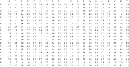
Dayhoff matrix. Each entry is a mutation probability from one amino acid (in rows) to another amino acid (in columns). Reproduced from [14] with permission.

Fig. 9.6.

The bio-basis function. As IPRS is more similar to KPRT than YKAE, its similarity with KPRT is larger that that with YKAE, see the right figure. Reproduced from [14] with permission.

The bio-basis function method has been successfully applied to various peptide classification tasks, for instance, the prediction of trypsin cleavage sites [9], the prediction of HIV cleavage sites [10], the prediction of hepatitis C virus protease cleavage sites [16], the prediction of the disorder segments in proteins [7, 17], the prediction of protein phosphorylation sites [18, 19], the prediction of the O-linkage sites in glycoproteins [20], the prediction of signal peptides [21], the prediction of factor Xa protease cleavage sites [22], the analysis of mutation patterns of HIV-1 drug resistance [23], the prediction of caspase cleavage sites [24], the prediction of SARS-CoV protease cleavage sites, [25] and T-cell epitope prediction [26].

Peptide Machines

As one class of machine learning approaches, various vector machines are playing important roles in machine learning research and applications. Three vector machines—the support vector machine [27, 28], relevance vector machine [29], and orthogonal vector machine [30]—have already drawn the attention for peptide bioinformatics. Each studies pattern classification with a specific focus. The support vector machine (SVM) searches for data points located on or near the boundaries for maximizing the margin between two classes of data points. These found data points are referred to as the support vectors. The relevance vector machine (RVM), on the other hand, searches for data points as the representative or prototypic data points referred to as the relevance vectors. The orthogonal vector machine (OVM) searches for the orthogonal bases on which the data points become mutually independent from each other. The found data points are referred to as the orthogonal vectors. All these machines need numerical inputs. We then see how to embed the bio-basis function into these vector machines to derive peptide machines.

Support Peptide Machine

The support peptide machine(SPM) aims to find a mapping function between an input peptide s and the class membership (functional status). The model is defined as

(2)

where w is the parameter vector, y = f(s, w) the mapping function, and y the output corresponding to the desired class membership t ∈ {–1, 1}. Note that –1 and 1 represent nonfunctional and functional status, respectively. With other classification algorithms like neural networks, the distance (error) between y and t is minimized to optimize w. This can lead to a biased hyperplane for discrimination. In Fig. 9.7, there are two classes of peptides, A and B. The four open circles of class A and four filled circles of the class B are distributed in balance. With this set of peptides, the true hyperplane separating two classes of peptides, represented as circles, can be found as in Fig. 9.7(a). Suppose a shaded large circle belonging to class B as a noise peptide is included, as seen in Fig. 9.7(b); the hyperplane (the broken thick line) is biased because the error (distance) between the nine circles and the hyperplane has to be minimized. Suppose a shaded circle belonging to class A as a noise peptide is included as seen in Fig. 9.7(c); the hyperplane (the broken thick line) also is biased. With theses biased hyperplanes, the novel peptides denoted by the triangles could be misclassified.

Fig. 9.7.

a Hyperplane formed using conventional classification algorithms for peptides with a balanced distribution. b and c Hyperplanes formed using conventional classification algorithms for peptides without balanced distribution. d Hyperplane formed using SPM for peptides without balanced distribution. The open circles represent class A, the filled circles class B, and the shaded circle class A or B. The thick lines represent the correct hyperplane for discrimination and the broken thick lines the biased hyperplanes. The thin lines represent the margin boundaries. The γ indicates the distance between the hyperplane and the boundary formed by support peptides. The margin is 2γ. Reproduced from [14] with permission.

In searching for the best hyperplane, the SPM finds the set of peptides that are the most difficult training data points to classify. These peptides are referred to as support peptides. In constructing a SPM classifier, the support peptides are closest to the hyperplane within the slat formed by two boundaries (Fig. 9.7d) and are located on the boundaries of the margin between two classes of peptides. The advantage of using an SPM is that the hyperplane is searched through maximizing this margin. Because of this, the SPM classifier is robust; hence, it has better generalization performance than neural networks. In Fig. 9.7(d), two open circles on the upper boundary and two filled circles on the lower boundary are selected as support peptides. The use of these four circles can form the boundaries of the maximum margin between two classes of peptides. The trained SPM classifier is a linear combination of the similarity between an input peptide and the found support peptides. The similarity between an input peptide and the support peptides is quantified by the bio-basis function. The decision is made using the following equation, y = sign {Σw _i t _i K(s, r _i)}, where t _i is the class label of the ith support peptide and w _i the positive parameter as a weight for the ith support peptide. The weights are determined by a SPM algorithm [31].

Relevance Peptide Machine

The relevance peptide machine (RPM) was proposed based on automatic relevance determination (ARD) theory [32]. In SPM, the found support peptides are normally located near the boundary for discrimination between two classes of peptides. However, the relevance peptides found by RPM are prototypic peptides. This is a unique property of RPM, as the prototypic peptides found by a learning process are useful for exploring the biological inside. Suppose the model output is defined as

(3)

where k _i = [K(s _i, r ₁), K(s _i, r ₂),..., K(s _i, r _m)]^T is a similarity vector and w = (w ₁, w ₂,..., w _n)^T. The model likelihood function is defined as follows:

(4)

Using ARD prior to computation can prevent overfitting the coefficients by assuming each weight follows a Gaussian

(5)

where α = (α₁, α₂,... , α_n)^T. The Bayesian learning method gives the following posterior for the coefficients:

(6)

where the parameters (covariance matrix Σ, the mean vector u, and the hyperparameters for weights S), which can be approximated:

(7)

(8)

(9)

(10)

and

(11)

The marginal likelihood can be obtained through integrating out the coefficients:

(12)

In learning, α can be estimated in an iterative way:

(13)

where

(14)

A formal learning process of the RPM is then conducted. The following condition is checked during learning:

(15)

where θ is a threshold. If the condition is satisfied, the corresponding expansion coefficient is zeroed. The learning continues until either the change of the expansion coefficients is small or the maximum learning cycle is approached [33].

Figure 9.8 shows how the RPM selects prototypic peptides as the relevance peptides, compared with the SPM, which selects boundary peptides as the support peptides.

Fig. 9.8.

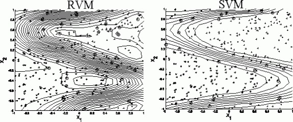
How RPM and SPM select peptides as relevance or support peptides. Note that this is only an illustration. The curves are contours. The crosses represent one class of peptides and the stars the other. The circles represent the selected data points as the relevance peptides for the RPM and the support peptides for theSPM.

Orthogonal Peptide Machine

First, we define a linear model using the bio-basis function as

(16)

where K is defined in Eq. 10. The orthogonal least square algorithm is used as a forward selection procedure by the orthogonal peptide machine (OPM). At each step, the incremental information content of a system is maximized. We can rewrite the design matrix K as a collection of column vectors (k ₁, k ₂,... , k _m), where k _i represents a vector of the similarities between all the training peptides and the ith indicator peptide r _i, k _i = [K(s ₁, r _i), K(s ₂, r _i),..., K(s _n, r _i)]^T. The OPM involves the transformation of the indicator peptides (r _i) to the orthogonal peptides (o _i) to reduce possible information redundancy. The feature matrix K is decomposed to an orthogonal matrix and an upper triangular matrix as follows:

(17)

where the triangular matrix U has ones on the diagonal line:

(18)

and the orthogonal matrix O is

(19)

The orthogonal matrix satisfies

(20)

where H is diagonal with the elements h _ii as

(21)

The space spanned by the set of orthogonal peptides is the same space spanned by the set of indicator peptides, and Eq. 16 can be rewritten as

(22)

We can define an error model as follows:

(23)

Suppose e ~ N(0, 1), the pseudoinverse method can be used to estimate a as follows:

(24)

Because H is diagonal,

(25)

The element in a is then

(26)

The quantities a and w satisfy the triangular system

(27)

The Gram-Schmidt or the modified Gram-Schmidt methods are commonly used to find the orthogonal peptides then to estimate w [30, 34].

Case Study: Drug Resistance Data Analysis

HIV/AIDS is one of the most lethal and transmittable diseases, with a high mortality rate worldwide. The most effective prevention of HIV infection is to use a vaccine to block virus infection [34]. However, HIV vaccine is difficult to develop because of the expense and complexity in advancing new candidate vaccines. Although some efficient models and integrated HIV vaccine research enterprises have been proposed [36], there is little hope that an HIV vaccine would be developed before 2009 [37]. HIV is a type of retrovirus. It can enter uninfected cells to replicate itself. Inhibiting viral maturation and viral reverse transcription are then the major methods so far for treating HIV-infected patients. Two groups of inhibitors have since been developed. One group aims to stop protease cleavage activities and is referred to as the protease inhibitor. The other aims to stop reverse transcriptase cleavage activities and is referred to as the reverse transcriptase inhibitor.

However, HIV often develops resistance to the drugs applied. Drug-resistant mutants of HIV-1 protease limit the long-term effectiveness of current antiviral therapy [38]. The emergence of drug resistance remains one of the most critical issues in treating HIV-1-infected patients [39]. The genetic reason for drug resistance is the high mutation rate along with a very high replication rate of the virus. These two factors work together, leading to the evolution of drug-resistant variants and consequently resulting in therapy failure. The resistance to HIV-1 protease inhibitors can be analyzed at a molecular level with a genotypic or a phenotypic method [39, 40]. The genotypic method is used to scan a viral genome for some mutation patterns for potential resistance. As an alternative, the viral activity can be measured in cell culture assays. Yet another alternative, phenotypic testing is based on clinic observations, ithat is, directly measuring viral replication in the presence of increasing drug concentration.

Genotypic assays have been widely used as tools for determining HIV-1 drug resistance and for guiding treatment. The use of such tools is based on the principle that the complex impact of amino acid substitutions in HIV reverse transcriptase or protease on the phenotypic susceptibility or clinical response to the 18 available antiretroviral agents is observable [41]. Genotypic assays are used to analyze mutations associated drug resistance or reduced drug susceptibility. However, this method is problematic, because various mutations and mutational patterns may lead to drug resistance [39], and therefore the method occasionally fails to predict the effects of multiple mutations [42]. In addition, genotypic assays provide only indirect evidence of drug resistance [43]. Although HIV-1 genotyping is widely accepted for monitoring antiretroviral therapy, how to interpret the mutation pattern associated with drug resistance to make accurate predictions of susceptibility to each antiretroviral drug is still challenging [44]. Phenotypic assays directly measure drug resistance [43], where drug resistance can be experimentally evaluated by measuring the ratio of free drug bound to HIV-1 protease molecules. However, this procedure is generally expensive and time consuming [39, 42].

To deal with the difficulties encountered in genotypic assay analysis and phenotypic evaluation, a combination of inhibitor flexible docking and molecular dynamics simulations was used to calculate the protein-inhibitor binding energy. From this, an inhibitory constant is calculated for prediction [39]. Later, some statistical models were established for predicting drug resistance. For instance, a statistical model was proposed to analyze the viral and immunologic dynamics of HIV infection, taking into account drug-resistant mutants and therapy outcomes [45]. The factors causing the increase in CD4 cell count and the decrease in viral load from baseline after six months of HAART (highly active antiretroviral therapy) were analyzed. Note that CD4 stands for cluster of differentiation 4, which is a molecule expressed on the surface of T helper cells. In addition to the baseline viral load and CD4 cell count, which are known to affect response to therapy, the baseline CD8 cell count and resistance characteristics of detectable strains are shown to improve prediction accuracy. Note that CD8 stands for cluster of differentiation 8, which is a membrane glycoprotein found primarily on the surface of cytotoxic T cells. A logistic regression model was built for the prediction of the odds of achieving virology suppression after 24 weeks of HAART in 656 antiretroviral-naive patients starting HAART according to their week 4 viral load [46]. A regression model was built on a set of 650 matched genotype-phenotype pairs for the prediction of phenotypic drug resistance from genotypes [47]. As it was observed that the range of resistance factors varies considerably among drugs, two simple scoring functions were derived from different sets of predicted phenotypes. The scoring functions were then used for discrimination analysis [48].

In addition, machine learning algorithms were used. Decision trees as a method for mimicking human intelligence were implemented to predict drug resistance [43]. A fuzzy prediction model was built based on a clinical data set of 231 patients failing highly active antiretroviral therapy (HAART) and starting salvage therapy with baseline resistance genotyping and virological outcomes after three and six months [49]. In the model, a set of rules predicting genotypic resistance was initially derived from an expert and implemented using a fuzzy logic approach. The model was trained using the virological outcomes data set, that is, Stanford's HIV drug-resistance database (Stanford HIVdb). Expert systems were also used for this purpose [41]. Neural networks as a type of powerful nonlinear modelers were utilized to predict HIV drug resistance for two protease inhibitors, indinavir and saquinavir [50].

Other than using sequence information for prediction, a structure-based approach was proposed to predict drug resistance [42]. Models of WT complexes were first produced from crystal structures. Mutant complexes were then built by amino acid substitutions in the WT complexes with subsequent energy minimization of the ligand (a small molecule binding to a protein or receptor) and PR (protease receptor) binding site residues. A computational model was then built based on the calculated energies.

The data set studied was obtained from an online relational database, the HIV RT and protease database (http://hivdb.stanford.edu) [51]. The susceptibility of the data to five protease inhibitors were determined, saquinavir (SQV), indinavir (IDV), ritonavir (RTV), nelfinavir (NFV) and amprenavir (APV). We obtained 255 genotype-phenotype pairs for each of the protease inhibitor, except for APV, for which we obtained 112 pairs. Phenotypic resistance testing measures in-vitro viral replication of the wild type and the viral sample in increasing drug concentrations [52]. The resistance factor, defined as the ratio of 50% inhibitory concentration (IC₅₀) of the respective viral sample to IC₅₀ of the nonresistant reference strain, reports the level of resistance as the fold change in susceptibility to the drug as compared to a fully susceptible reference strain. While genotypic resistance testing is done by scanning the viral genome for resistance-associated mutations. The major and minor mutations observed in a resistant HIV protease can be seen in Figure 1 in [53]. HIV protease is an aspartyl protease with 99 residues. In this study, we considered major and minor mutation sites, obtaining a window size of 20 residues for each drug. We divided the sample set into two classes by attaching to each peptide a label 1 or –1 for resistant (functional) and susceptible (nonfunctional), respectively. This division depended on whether the resistance factor of a sample exceeded the cutoff value or not. Based on previously published datasets and studies, we assumed the cutoff value for the resistant factor of each sample with respect to each protease inhibitor to be 3.5.

We used Matthews correlation coefficient [54] for evaluation. Let TN, TP, FN, and FP denote true negative, true positive, false negative, and false positive, respectively. The definition of the Matthews correlation coefficient (MCC) is

(28)

The larger the Matthews correlation coefficient, the better the model fits the target. If the value of the Matthews correlation coefficient is 1, it represents a complete correlation. If the value is 0, the prediction is completely random. If the value is negative, the prediction is on the opposite side of the target.

The evaluation is carried out based on the simulation of fivefold cross-validation for each drug and each algorithm. Figure 9.9 shows the comparison between vector machines and peptide machines. It can be seen that the peptide machines outperformed the vector machines. We also constructed neural networks models for this task, their performance is far worse than vector machines (data are not shown).

Fig. 9.9.

Comparison between two vector machines and three peptide machines. The three peptide machines outperformed the two vector machines.

Practical Issues in Peptide Classification

In building a computer model for a real application, there are two important issues for model validation in addition to model parameter estimation. The first is how to evaluate a model. The second is how to select a model based on the evaluation. There are always some hyperparameters for determination when using neural networks or machine learning algorithms. For instance, the number of hidden neurons in feedforward neural networks is such a hyperparameter, and the determination of the number of hidden neurons is not an easy task. Using the training data for the evaluation will not deliver meaningful result, as an optimization process can easily overfit the data, leading to poor generation capability. The generalization capability measures how well a built model works with novel data.

Based on this requirement, we then need to consider how to use the available data for proper model validation. There are three commonly used methods for this purpose: cross-validation, resampling, and jackknife. All these methods use the same principle, that the validation data must not involve any process of model parameter estimation. This means that the available data must be divided into two parts. One is for model parameter estimation, which is commonly referred to as training. The other is for model evaluation (validation) and selection. The difference between these three methods is the strategy used for the division of a given data set.

Resampling

With the resampling method, we normally randomly sample a certain percentage of data for training and the rest for validation. Such a process is commonly repeated many times. Suppose there are n data points and we repeat the sampling process for m times. There will be m validation models, each of which has different training and validation data with some possible overlap. Note that all these validation models use the same hyperparameters; for instance, they all use h hidden neurons. The parameters of the ith validation model are estimated using the ith training data set with k _i < n data points. The ith validation model is validated on the ith validation data set with n – k _i data points. Because we use different training data sets each time, it is expected that the parameters of the ith validation model will be different from those of the jth validation model. The validation performance of the ith validation model is certainly different from that of the jth validation model as well. We denote by the evaluated performance for the ith validation model. The evaluation statistic of the model with designed hyperparameters can follow

(29)

To determine the proper values for the hyperparameters, so that we can select a proper model, we can vary the values assigned to the hyperparameters. If we have g hyperparameters for selection, the selection will be taken in a g-dimensional space, where each grid is a combination of hyperparameters. Suppose we need to determine only the number of hidden neurons, we then have a series of and . The best model can be selected through

(30)

It should be noted that, for the resampling method, some data points may be used for multiple times in training or validation.

Cross-Validation

In cross-validation, we normally randomly divide a data set into m folds. Each fold contains distinctive data points. If we denote by Ω_i as the set of data points in ith fold, we have Ω_i ∩ Ω_j = φ, meaning that two sets have no elements in common. Every time, we select one fold as the validation set and the remaining m – 1 folds are used as the training set for model parameters estimate. Such a process is repeated for m times, until each fold has been used for validation once. This means that there are m validation models. Again, all these validation models use the same hyperparameters. The ith validation model is trained using the folds except for the ith fold and validated on the ith fold. The parameters of the ith validation model also is different from those of the jth validation model, and the validation performance of different validation models will vary. Note that each data point ise validated only once. We denote by the evaluated performance for the ith data point. The evaluation of the model with designed hyperparameters can follow

(31)

Suppose we need to determine only the number of hidden neurons, we then have a series of and . The best model can be selected through the use of Eq. 30.

Jackknife

When data size is not too large, one commonly prefers using the jackknife (often called leave-one-out cross-validation) method. In using the jackknife method, we normally pick up one data point for validation and use the remaining data points for training. Such a process is repeated for n times until each data point has been exhausted for validation. This means that there are n validation models for n data points. Obviously, all these validation models use the same hyperparameters. The ith validation model is trained using all the data points except for the ith data point and validated on the ith data point. Equation 31 can be used for evaluation. The best model can be selected through the use of Eq. 30.

Blind Test

Model validation can help us evaluate models and select models with a proper setting of hyperparameters. However, such evaluation values cannot be regarded as the final model evaluation, which can be delivered to users. The evaluated performance on validation data may not be able to reflect the true performance, because the validation data has been used to tune hyperparameters. As a consequence, the evaluated performance on validation data commonly overestimates the true model accuracy.

Based on this understanding, a proper peptide classification methodology must contain a blind test stage. This means that, after model evaluation and model selection, we may need to test the “best” model using another data set, which has never been used for estimating model parameters and tuning model hyperparameters or selecting models [7].

Protein-Oriented Validation

A very important issue must be discussed here, especially for peptide classification. Many peptide classification tasks deal with functional site predictions. Within each protein sequence, there might be a few functional sites, such as protease cleavage sites, protein interaction sites, or protein posttranslational modification sites. Based on the substrate size, we can extract a peptide around one functional site. Such a peptide is commonly regarded as a functional peptide. To conduct proper peptide classification, we have to have a set of nonfunctional peptides. Each nonfunctional peptide has no functional site at the desired residue(s). We normally use a sliding window with a fixed length to scan a protein sequence from the N-terminal to the C-terminal, one residue by one residue to generate no-functional peptides. A commonly used method is to combine both functional and nonfunctional peptides to produce a data set. Suppose we use the cross-validation method, the data set is then randomly divided into m folds for cross-validation. One then builds m validation models for model evaluation and model selection. Now a question arises. When we use such kind of models for testing on novel whole protein sequences, the performance is commonly not as expected. This means that the model is some where overfitted. If model parameter estimation follows a proper procedure, the most probable problem is the data used for training and validation. We mentioned previously that we must maintain the independence of a validation data set from a training data set. When we check the method as described, we can clearly see two interesting facts. First, a training peptide and a validation peptide may come from the same protein. If one protein has conserved amino acids, the validation peptides generated this way may not be independent of the training peptides. Second, a training peptide and a validation peptide may have many identical residues if they are extracted from neighboring sliding widows.

Based on this analysis, we proposed to use protein-oriented validation [24]. Suppose we have n proteins, we may divide these n proteins into m folds. We then generate validation peptides using one fold and generate training peptides from the remaining folds. The validation models are constructed using the training peptides scanned from the sequences of the training proteins and verified on the validation peptides scanned from the sequences of the validation proteins.

Model Lifetime

We always have an important issue when using machine learning approaches for peptide classification, That is, if the model is correct forever. The answer is no, as a peptide data set collected at a certain time can be far less than complete. Based on this understanding, the models built using an incomplete set of peptides may not be able to generalize well forever. When new experimentally determined peptides have been collected, the exiting models must be corrected so that they can conduct classification tasks well. In this section, we investigate an interesting peptide classification topic, where we can use a model built on published peptides for peptide classification, and we can use a model built on both published peptides and newly submitted sequences in NCBI (www.ncbi.nih.gov) for peptide classification. We found there is a significant difference between the two.

The case studied in this session is about hepatitis C virus (HCV), which is a member of the flaviviridae family [55] and is the major agent of parenterally transmitted non-A/non-B hepatitis [56, 57]. The nomenclature of Schechter and Berger [1] is applied to designate the cleavage sites on the peptides, P₆-P₅-P₄-P₃-P₂-P₁-P_1'-P_2'-P_3'-P_4', the asymmetric scissile bond being between P₁ and P_1'. Two resources are available for modeling. First, research articles have published experimentally determined peptides, cleaved and noncleaved. Second, some databank like NCBI has collected many new submissions. Each submission contains a whole protein sequence with a number of experimentally determined cleavage sites. In terms of this, there are two strategies for modeling. If we believe that the published peptides are able to represent all the protease cleavage specificity, we can select indicator peptides from these published peptides for modeling. We refer to a model constructed this way as a Type-I model. In fact, viruses mutate very rapidly; hence, the published peptides may not be able to represent the cleavage specificity in the recent submissions to NCBI. We can then select more indicator peptides, which show more viral mutation information from the new sequences downloaded from NCBI to build a more informative model referred to as a Type-II model.

From published papers (data are not shown), we collected 215 experimentally determined peptides. They are referred to as published peptides in this study. Among them, 168 are cleaved, while 47 are noncleaved. Twenty-five whole protein sequences were downloaded from NCBI. They are aaa65789, aaa72945, aaa79971, aab27127, baa01583, baa02756, baa03581, baa03905, baa08372, baa09073, baa09075, baa88057, bab08107, caa03854, caa43793, cab46677, gnwvtc, jc5620, np_043570, np_671491, p26663, p26664, p27958, pc2219, and s40770. Within these 25 whole protein peptides (data are not shown) are 123 cleavage sites. The cleavage sites with notes of potential, by similarity, or probable were removed.

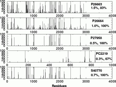
First, we built Type-I models using the leave-one-out method. Each model is built on 214 published peptides and tested on 1 remaining published peptide. The models are then evaluated in terms of the mean accuracy, which is calculated on 215 leave-one-out testes. The best model is selected and tested on 25 new sequences downloaded from NCBI, which are regarded as the independent testing data. The simulation shows that the noncleaved, cleaved, and total accuracies are 77%, 77%, and 77%, respectively. Shown in Fig. 9.10 are the prediction results on five whole protein sequences, where the horizontal axis indicates the residues in whole protein sequences and the vertical axis the probability of positive (cleavage). If the probability at a residue is larger than 0.5, the corresponding residue is regarded as the cleavage site P₁. The simulation shows that there were too many false positives. The average of false positive fraction was 27%, or 722 misclassified noncleavage sites.

Fig. 9.10.

The probabilities of cleavage sites among the residues for five whole protein sequences for the Type-I models. The horizontal axes indicate the residues in the whole sequences and the vertical axes the probabilities of positives (cleavage sites). The numbers above the percentages are the NCBI accession numbers and the percentages are the false-positive fractions and the true- positive fractions. Reproduced from [58] with permission.

Second, we built Type-II models. Each model is built and validated using all the published peptides (215) plus the peptides scanned from 24 newly downloaded sequences. In this run, the protein-oriented leave-one-out method is used. With this method, 1 of 24 new sequences is removed for validation on a model built using 215 published peptides and the peptides scanned from the remaining 23 new sequences. This is repeated 24 times and the performance is estimated on the predictions on 24 new sequences. The best model is selected and tested on the peptides on the remaining new sequence. These peptides are regarded as the independent testing peptides. The noncleaved, cleaved, and total accuracies are 99%, 83%, and 99%, respectively. It can be seen that the prediction accuracy has been greatly improved compared with the Type-I models. Shown in Fig. 9.11 is a comparison between the Type-I and the Type-II models. It shows that the Type-II models greatly outperformed the Type-I models in terms of the performance for noncleaved peptides. More important, the standard deviation in the Type-II models is much smaller, demonstrating high robustness.

Fig. 9.11.

A comparison between the Type-I and Type-II models. It can be seen that the Type-II models performed much better than the Type-I models in terms of the increase of specificity (true-negative fraction). Therefore, the false-positive fraction (false alarm) has been significantly reduced. TNf and TPf stand for true-negative fraction (specificity) and true-positive fraction (sensitivity). Reproduced from [58] with permission.

Shown in Fig. 9.12 are the prediction results on five protein sequences using the Type-II models, where the horizontal axis indicates the residues in whole protein sequences and the vertical axis the probability of positive (cleavage). The simulation shows fewer false positives than the Type-I models. The reason is that many of the 25 newly downloaded sequences were published after the reports with the published peptides. The published peptides may not contain complete information for all these 25 new sequences.

Fig. 9.12.

The probabilities of cleavage sites among the residues for five whole protein sequences for the Type-II models. The horizontal axes indicate the residues in whole sequences and the vertical axes the probabilities of positives (cleavage sites). The numbers above the percentages are the NCBI accession numbers and the percentages are the false positive fractions and the true positive fractions. The simulation shows that the Type-II models demonstrated very small false-positive fractions compared with the Type-I models. It can be seen that the probability of positives are very clean. Reproduced from [58] with permission.

Summary and Future Work

This chapter introduced the state-of-the-art machines for peptide classification. Through the discussion, we can see the difference between the peptide machines and other machine learning approaches. Each peptide machine combines the feature extraction process and the model construction process to improve the efficiency. Because peptide machines use the novel bio-basis function, they can have biologically well-coded inputs for building models. This is the reason that the peptide machines outperformed the other machine learning approaches. The chapter also discussed some issues related with peptide classification, such as model evaluation, protein-oriented validation, and model lifetime. Each of these issues is important in terms of building correct, accurate, and robust peptide classification models. For instance, the blind test can be easily missed by some new bioinformatics researchers. Protein-oriented validation has not yet been paid enough attention in bioinformatics. There is also little discussion on model lifetime. Nevertheless, these important issues have been evidenced in this chapter.

We should note that there is no a priori knowledge about which peptide machine should be used. Research into the link between these three peptide machines may provide some important insights for building better machines for peptide classification. The core component of peptide machines is a mutation matrix. Our earlier work shows that the model performance using various mutation matrices varies [10]. It is then interesting to see how we can devise a proper learning method to optimize the mutation probabilities between amino acids during model construction.

References

- 1.Schechter I, Berger A. On the active site of proteases, 3. Mapping the active site of papain; specific peptide inhibitors of papain. Biochem Biophys Res Comms. 1968;32:898. doi: 10.1016/0006-291X(68)90326-4. [DOI] [PubMed] [Google Scholar]
- 2.Blom N, Gammeltoft S, Brunak S. Sequence and structure based prediction of eukaryotic protein phosphorylation sites. J Mol Biol. 1999;294:1351–1362. doi: 10.1006/jmbi.1999.3310. [DOI] [PubMed] [Google Scholar]
- 3.Kobata A. The carbohydrates of glycoproteins. In: Ginsburg V, Robins PW (eds), editors. Biology of carbohydrates. New York: Wiley; 1984. [Google Scholar]
- 4.Yang ZR, Wang L, Young N, Trudgian D, Chou KC. Machine learning algorithms for protein functional site recognition. Current Protein and Peptide Science. 2005;6:479–491. doi: 10.2174/138920305774329322. [DOI] [PubMed] [Google Scholar]
- 5.Dunker AK, Obradovic Z, Romero P, Garner EC, Brown CJ. Intrinsic protein disorder in complete genomes. Genome Inform Ser Workshop Genome Inform. 2000;11:161–171. [PubMed] [Google Scholar]
- 6.Baldi P, Pollastri G, Andersen C, Brunak S. Matching protein beta-sheet partners by feedforward and recurrent neural networks. Proceedings of International Conference on Intelligent Systems for Molecular Biology. ISMB. 2000;8:25–36. [PubMed] [Google Scholar]
- 7.Yang ZR, Thomson R, McNeil P, Esnouf R. RONN: use of the bio-basis function neural network technique for the detection of natively disordered regions in proteins. Bioinformatics. 2005;21:3369–3376. doi: 10.1093/bioinformatics/bti534. [DOI] [PubMed] [Google Scholar]
- 8.Qian N, Sejnowski TJ. Predicting the secondary structure of globular proteins using neural network models. J Molec Biol. 1988;202:865–884. doi: 10.1016/0022-2836(88)90564-5. [DOI] [PubMed] [Google Scholar]
- 9.Thomson R, Hodgman TC, Yang ZR, Doyle AK. Characterising proteolytic cleavage site activity using bio-basis function neural networks. Bioinformatics. 2003;19:1741–1747. doi: 10.1093/bioinformatics/btg237. [DOI] [PubMed] [Google Scholar]
- 10.Yang ZR, Thomson R. A novel neural network method in mining molecular sequence data. IEEE Trans on Neural Networks. 2005;16:263–274. doi: 10.1109/TNN.2004.836196. [DOI] [PubMed] [Google Scholar]
- 11.Altschul SF, Gish W, Miller W, Myers E, Lipman DJ. Basic local alignment search tool. J. Molec. Biol. 1990;215:403–410. doi: 10.1016/S0022-2836(05)80360-2. [DOI] [PubMed] [Google Scholar]
- 12.Dayhoff MO, Schwartz RM, Orcutt BC 1978 A model of evolutionary change in proteins. matrices for detecting distant relationships. In: Dayhoff MO (ed) Atlas of protein sequence and structure, vol. 5, pp.345–358.
- 13.Johnson MS, Overington JP. A structural basis for sequence comparisons—an evaluation of scoring methodologies. J Mol Biol. 1993;233:716–738. doi: 10.1006/jmbi.1993.1548. [DOI] [PubMed] [Google Scholar]
- 14.Yang ZR. Application of support vector machines to biology. Briefings in Bioinformatics. 2004;5:328–338. doi: 10.1093/bib/5.4.328. [DOI] [PubMed] [Google Scholar]
- 15.Edelman J, White SH. Linear optimization of predictors for secondary structure: application to transbilayer segments of membrane proteins. J Mole Biol. 1989;210:195–209. doi: 10.1016/0022-2836(89)90300-8. [DOI] [PubMed] [Google Scholar]
- 16.Yang ZR, Berry E. Reduced bio-basis function neural networks for protease cleavage site prediction. J Comput Biol Bioinformatics. 2004;2:511–531. doi: 10.1142/S0219720004000715. [DOI] [PubMed] [Google Scholar]
- 17.Thomson R, Esnouf R. Predict disordered proteins using bio-basis function neural networks. Lecture Notes in Computer Science. 2004;3177:19–27. doi: 10.1007/978-3-540-28651-6_16. [DOI] [Google Scholar]
- 18.Berry E, Dalby A, Yang ZR. Reduced bio basis function neural network for identification of protein phosphorylation sites: comparison with pattern recognition algorithms. Comput Biol Chem. 2004;28:75–85. doi: 10.1016/j.compbiolchem.2003.11.005. [DOI] [PubMed] [Google Scholar]
- 19.Senawongse P, Dalby AD, Yang ZR. Predicting the phosphorylation sites using hidden Markov models and machine learning methods. J Chem Info Comp Sci. 2005;45:1147–1152. doi: 10.1021/ci050047+. [DOI] [PubMed] [Google Scholar]
- 20.Yang ZR, Chou KC. Bio-basis function neural networks for the prediction of the O-linkage sites in glyco-proteins. Bioinformatics. 2004;20:903–908. doi: 10.1093/bioinformatics/bth001. [DOI] [PubMed] [Google Scholar]
- 21.Sidhu A, Yang ZR. Predict signal peptides using bio-basis function neural networks. Applied Bioinformatics. 2006;5(1):13–19. doi: 10.2165/00822942-200605010-00002. [DOI] [PubMed] [Google Scholar]
- 22.Yang ZR, Dry J, Thomson R, Hodgman C. A bio-basis function neural network for protein peptide cleavage activity characterisation. Neural Networks. 2006;19:401–407. doi: 10.1016/j.neunet.2005.07.015. [DOI] [PubMed] [Google Scholar]
- 23.Yang ZR, Young N. Bio-kernel self-organizing map for HIV drug resistance classification. Lecture Notes in Computer Science. 2005;3610:179–184. doi: 10.1007/11539087_20. [DOI] [Google Scholar]
- 24.Yang ZR. Prediction of caspase cleavage sites using Bayesian bio-basis function neural networks. Bioinformatics. 2005;21:1831–1837. doi: 10.1093/bioinformatics/bti281. [DOI] [PubMed] [Google Scholar]
- 25.Yang ZR. Mining SARS-coV protease cleavage data using decision trees, a novel method for decisive template searching. Bioinformatics. 2005;21:2644–2650. doi: 10.1093/bioinformatics/bti404. [DOI] [PMC free article] [PubMed] [Google Scholar]
- 26.Yang ZR, Johnathan F. Predict T-cell epitopes using bio-support vector machines. J Chem Inform Comp Sci. 2005;45:1142–1148. [Google Scholar]
- 27.Vapnik V. The nature of statistical learning theory. New York: Springer-Verlag; 1995. [Google Scholar]
- 28.Scholkopf B (2000) The kernel trick for distances. Technical report, Microsoft Research, May.
- 29.Tipping ME. Sparse Bayesian learning and the relevance vector machine. J Machine Learning Res. 2001;1:211–244. doi: 10.1162/15324430152748236. [DOI] [Google Scholar]
- 30.Chen S, Cowan CFN, Grant PM. Orthogonal least squares learning algorithm for radial basis function networks. IEEE Trans on Neural Networks. 1991;2:302–309. doi: 10.1109/72.80341. [DOI] [PubMed] [Google Scholar]
- 31.Yang ZR, Chou KC. Bio-support vector machines for computational proteomics. Bioinformatics. 2003;19:1–7. doi: 10.1093/bioinformatics/19.1.1. [DOI] [PubMed] [Google Scholar]
- 32.MacKay DJ. A practical Bayesian framework for backpropagation networks. Neural Computation. 1992;4:448–472. doi: 10.1162/neco.1992.4.3.448. [DOI] [Google Scholar]
- 33.Yang ZR. Orthogonal kernel machine in prediction of functional sites in proteins. IEEE Trans on Systems. Man and Cybernetics. 2005;35:100–106. doi: 10.1109/TSMCB.2004.840723. [DOI] [PubMed] [Google Scholar]
- 34.Yang ZR, Thomas A, Young N, Everson R (2006) Relevance peptide machine for HIV-1 drug resistance prediction. IEEE Trans on Computational Biology and Bioinformatics (in press).
- 35.Putney S. How antibodies block HIV infection: paths to an AIDS vaccine. Trends in Biochem Sci. 1992;7:191–196. doi: 10.1016/0968-0004(92)90265-B. [DOI] [PubMed] [Google Scholar]
- 36.Klausner RD, et al. The need for a global HIV vaccine enterprise. Science. 2003;300:2036–2039. doi: 10.1126/science.1086916. [DOI] [PubMed] [Google Scholar]
- 37.Kathryn S. HIV vaccine still out of our grasp. The Lancet Infectious Diseases. 2003;3:457. doi: 10.1016/s1473-3099(03)00705-9. [DOI] [PubMed] [Google Scholar]
- 38.Weber IT, Harrison RW. Molecular mechanics analysis of drug-resistant mutants of HIV protease. Protein Eng. 1999;12:469–474. doi: 10.1093/protein/12.6.469. [DOI] [PubMed] [Google Scholar]
- 39.Jenwitheesuk E, Samudrala R. Prediction of HIV-1 protease inhibitor resistance using a protein-inhibitor flexible docking approach. Antivir Ther. 2005;10:157–166. [PubMed] [Google Scholar]
- 40.Gallego O, Martin-Carbonero L, Aguero J, de Mendoza C, Corral A, Soriano V. Correlation between rules-based interpretation and virtual phenotype interpretation of HIV-1 genotypes for predicting drug resistance in HIV-infected individuals. J Virol Methods. 2004;121:115–118. doi: 10.1016/j.jviromet.2004.06.003. [DOI] [PubMed] [Google Scholar]
- 41.De Luca A, Cingolani A, et al. Variable prediction of antiretroviral treatment outcome by different systems for interpreting genotypic human immunodeficiency virus type 1 drug resistance. J Infect Dis. 2003;187:1934–1943. doi: 10.1086/375355. [DOI] [PubMed] [Google Scholar]
- 42.Shenderovich MD, Kagan RM, Heseltine PN, Ramnarayan K. Structure-based phenotyping predicts HIV-1 protease inhibitor resistance. Protein Sci. 2003;12:1706–1718. doi: 10.1110/ps.0301103. [DOI] [PMC free article] [PubMed] [Google Scholar]
- 43.Brenwinkel N, Schmidt B, Walter H, Kaiser R, Lengauer T, Hoffmann D, Korn K, Selbig J. Diversity and complexity of HIV-1 drug resistance: a bioinformatics approach to predicting phenotype from genotype. PNAS. 2002;99:8271–8276. doi: 10.1073/pnas.112177799. [DOI] [PMC free article] [PubMed] [Google Scholar]
- 44.Sturmer M, Doerr HW, Staszewski S, Preiser W. Comparison of nine resistance interpretation systems for HIV-1 genotyping. Antivir Ther. 2003;8:239–244. [PubMed] [Google Scholar]
- 45.Vergu E, Mallet A, Golmard JL. The role of resistance characteristics of viral strains in the prediction of the response to antiretroviral therapy in HIV infection. J Acquir Immune Defic Syndr. 2002;30:263–270. doi: 10.1097/00126334-200207010-00001. [DOI] [PubMed] [Google Scholar]
- 46.Smith CJ, Staszewski S, et al. Use of viral load measured after 4 weeks of highly active antiretroviral therapy to predict virologic putcome at 24 weeks for HIV-1-positive individuals. J Acquir Immune Defic Syndr. 2004;37:1155–1159. doi: 10.1097/01.qai.0000135958.80919.e4. [DOI] [PubMed] [Google Scholar]
- 47.Beerenwinkel N, Daumer M, et al. Geno2pheno: estimating phenotypic drug resistance from HIV-1 genotypes. Nucleic Acids Res. 2003;31:3850–3855. doi: 10.1093/nar/gkg575. [DOI] [PMC free article] [PubMed] [Google Scholar]
- 48.Foulkes AS, De GV. Characterizing the relationship between HIV-1 genotype and phenotype: prediction-based classification. Biometrics. 2002;58:145–156. doi: 10.1111/j.0006-341X.2002.00145.x. [DOI] [PubMed] [Google Scholar]
- 49.De Luca A, Vendittelli, et al. Construction, training and clinical validation of an interpretation system for genotypic HIV-1 drug resistance based on fuzzy rules revised by virological outcomes. Antivir Ther. 2004;9:583–593. [PubMed] [Google Scholar]
- 50.Draghici S, Potter RB. Predicting HIV drug resistance with neural networks. Bioinformatics. 2003;19:98–107. doi: 10.1093/bioinformatics/19.1.98. [DOI] [PubMed] [Google Scholar]
- 51.Shafer RW, Stevenson D, Chan B. Human immunodeficiency virus reverse transcriptase and protease sequence database. Nucleic Acids Res. 1999;27:348–352. doi: 10.1093/nar/27.1.348. [DOI] [PMC free article] [PubMed] [Google Scholar]
- 52.Walter H, Schmidt B, Korn K, Vandamme AM, Harrer T, Uberla K. Rapid, phenotypic HIV-1 drug sensitivity assay for protease and reverse transcriptase inhibitors. J Clin Virol. 1999;13:71–80. doi: 10.1016/S1386-6532(99)00010-4. [DOI] [PubMed] [Google Scholar]
- 53.Sa-Filho DJ, Costa LJ, de Oliveira CF, Guimaraes APC, Accetturi CA, Tanuri A, Diaz RS. Analysis of the protease sequences of HIV-1 infected individuals after indinavir monotherapy. J Clin Virology. 2003;28:186–202. doi: 10.1016/S1386-6532(03)00007-6. [DOI] [PubMed] [Google Scholar]
- 54.Matthews BW. Comparison of the predicted and observed secondary structure of T4 phage lysozyme. Biochim Biophys Acta. 1975;405:442–451. doi: 10.1016/0005-2795(75)90109-9. [DOI] [PubMed] [Google Scholar]
- 55.Francki R, Fauquet C, Knudson D, Brown F. Classification and nomenclature of virus: fifth report of the International Committee on Taxonomy of Viruses. Arch Virology. 1991;2:223s. [Google Scholar]
- 56.Choo Q, Kuo G, Weiner AJ, Overby L, Bradley D, Houghton M. Isolation of a cDNA clone derived from a blood-borne non-A non-B viral hepatitis genome. Science. 1989;244:359–362. doi: 10.1126/science.2523562. [DOI] [PubMed] [Google Scholar]
- 57.Kuo G, Choo Q, et al. An assay for circulating antibodies to a major etiologic virus of human non-A non-B hepatitis. Science. 1989;244:362–364. doi: 10.1126/science.2496467. [DOI] [PubMed] [Google Scholar]
- 58.Yang ZR. Predicting hepatitis C virus protease cleavage sites using generalised linear indicator regression models. IEEE Trans on Biomedical Engineering. 2006;53:2119–2123. doi: 10.1109/TBME.2006.881779. [DOI] [PubMed] [Google Scholar]