Highlights
-
•
Mathematical modeling of fractional SIS epidemic model.
-
•
The existence and uniqueness of the solution of this model.
-
•
The iterative solution with variational iteration method (VIM).
-
•
Numerical results with forward Euler method and variational iteration method for the fractional order SIS model.
-
•
The effect of the memory of the fractional system on its dynamic.
Keywords: Fractional order epidemic model, Fractional SIS model, Fractional forward euler method, Variational iteration method, Mittag leffler function
Abstract
We consider the fractional order epidemic model based on assumption that people will recover after disease and may be infected again on a time interval of non fatal disease. Our mathematical formulation is based on the fractional Caputo derivative. The existence and uniqueness of the solution is discussed. Furthermore, numerical solution is studied by variational iteration method and Euler method. Consequently, some numerical results are presented within.
1. Introduction
The formulation in mathematical language of a concrete phenomenon has aroused always arouses the curiosity of many mathematicians. This modeling dates from the time of Fibonacci (the growth of a rabbit populations). It can be said that the foundations of mathematical epidemiology are based on models of compartments, and the structure of epidemic models is determined by the flow of individuals from one compartment to another in a population. Hence, in the literature various models are proposed namely, a simple model is the susceptible-infected model, in the SI model individuals can be in two states susceptible (healthy) and infected, SIR model is the susceptible-infected-recovered model, it’s based on the assumption that an infected individual can recover after disease and can not be infected again, that is in contrast to SIS model in which individual can recover after disease and may be infected again and so on. The model prey-predator (1926), or model of Lotka-Volterra, plays a determinant role in dynamics of population and is considered as a basic conceptual model in population dynamics and also in mathematical epidemiology.
Fractional calculus as generalization of differentiation and integration of a function to arbitrary order has gained a considerable amount of interest by many authors, hence they have used this mathematical tool to describe many phenomenon with non local behavior (memory effect) in different areas of research.
In the classical integer order epidemic models, (SIS, SI or SIR models) the disease is transmitted with the same probability between compartments of the model studied, then rates of contact and transmission of disease are supposed to be constant, in other words, classical models ’state does not depend on its history, however, the state of evolution of epidemic depends not only upon its present state but also upon its past states, it’s related to the individual’s experiences, hence it’s more acceptable to study the evolution of an epidemic in a human society by taking into account the history of the system, virtually this could be possible by replacing the ordinary derivative by a fractional one, in fact the definition of any fractional derivation contains a memory kernel or memory function, expressing a system with such derivative makes every state of the system in study depend on past states, Saeedian M et al. explain in details the memory effects on epidemic evolution using fractional derivative [1], the reader can refer to this article and references cited there.
Various epidemic models have successful being proposed and studied as generalized of classical integers ones. The fractional SIR model have been first considered in 2000 [2], where Hethcote proposed a comprehensive analysis on the SIR model with a constant population, in the same year Driessche PVD and Watmough J presented a classical simple SIS model with a contact rate depending on time [3]. Moreover in 2014 the fractional order SIS model has been developed with a constant population size [4] and with a variable population size [5], in both works the stability of equilibrium points of the model is studied, two years later mathematical model for the transmission of Ebola in human society has been presented [6], in the same year Ameen I and Novati P proposed numerical solution for fractional SIR model with constant population [7] by using discrete methods: Generalized Euler Method and Predictor Corrector Adams method, which is an implicit numerical scheme, also Okyere E et al. studied a fractional order extension of the SIR and SIS model by replacing the ordinary derivative by the Caputo fractional derivative [8], they used also Adams method to illustrate model solutions and Banerjee SK studied a fractional order SIS epidemic model with constant recruitment rate and variable population size [9], in 2017 Sun GQ et al. suggested a mathematical model to describe the transmission of cholera in the population of China [10], what is particular in this model is the environment-to-human transmission of the disease, Li L presented a dynamical model on hemorrhagic fever with renal syndrome in China [11], within the same frame Ahmed EM and El-Saka HA studied the transmission of a dangerous epidemic, called MERS-CoV using fractional order derivative [12], recently in 2018 Sigh J et al. considered a fractional epidemiological SIR model to describe the spread of computer virus [13].
In the same area of research, some mathematical studies use recent analytic methods for solving fractional epidemic systems like the adomian decomposition method ADM [14], variational iterative method VIM [15], homotopy perturbation method HPM [16] and homotopy analysis method HAM [17], [18]. Those methods are powerful tools to provide rapidly convergent successive approximations of exact solution for non linear fractional problems. Mathematical epidemic compartment models have been studied by several researchers. For more details, the reader can refer to: [19], [20], [21], [22], [23].
The main objective of our work is to introduce the fractional-order approach for the study of particular SIS model in a constant population. In this case the fractional order system of the SIS model will be transformed to one fractional equation that describes the trajectory of infected individuals.
The paper is organized as follows: In Section 2, some basic results on fractional Caputo derivative are given. Section 3, is devoted to present the mathematical modeling of the ordinary SIS model. In Section 4, we introduce the fractional SIS model, in Section 5, we investigate existence and uniqueness of solution of the fractional system. Section 6, is devoted to describing the numerical methods that are used to solve the fractional SIS epidemic system, which is following in Section 7 by numerical solutions. Our paper is concluded by some comments and conclusion.
2. Some basic results on fractional Caputo derivative
In this section, we review some definitions and some results of fractional Caputo derivative. To get more details, the reader can refer to: [24], [25], [26], [27] for example.
The Caputo fractional derivative of order α is defined as
| (1) |
where with [α] is the integer part of the positive real number α.
The Riemann-Liouville fractional integral of order α is defined by
| (2) |
where is the order of integration, and
| (3) |
is the Euler Gamma function.
Caputo derivative and the Riemann-Liouville integral satisfy the following properties [24]
| (4) |
| (5) |
| (6) |
In this work, we study fractional differential system where 0 < α < 1, so the last formula becomes
| (7) |
3. Mathematical modeling of the ordinary SIS model
The evolution of this epidemic in a population of large size N is modeled by the following differential system [28]
| (8) |
where parameters e > 0, γ > 0 and β > 0 are respectively, the per death rate of infected, the healing rate and the contact rate. In the SIS model, the population in question is divided into two compartments: S(t) denotes susceptible individuals while I(t) is the infected individuals. In this model, a susceptible individual becomes infected and infectious after contact with an infectious individual, he becomes again susceptible to the rate γ (the cure rate). In this case, newborns are not infected and deaths are from compartment I. Hence, and the population is constant.
Since therefore, for all t ≥ 0, we obtain So, we have
| (9) |
We denote the ordinary differential equation satisfied by I, becomes
| (10) |
subject to the initial condition Hence, looking for solutions of the fractional differential Eq. (10) needs three cases to be discussed
- If and c ≠ 0 then, ∀t ≥ 0, we obtain by uniqueness of solution.
- If c = 0, the Eq. (10) becomes
| (11) |
subject to the initial condition Its solution is given by, ∀t ≥ 0,
| (12) |
- If and c ≠ 0 so, ∀t ≥ 0, we get
| (13) |
The ordinary classical SIS model obviously has these limits because the epidemiological parameters e, β and γ could change along the experiment, they depend on the past of the experiment, of which the ordinary model assumes that disease spreads in a linear manner, which is not always true. The real understanding of this epidemic is crucial. To do this, we propose the fractional model.
4. Mathematical modeling of the fractional SIS model
The fractional model of the actual evolution of this epidemic in a population of large size N is given by the following fractional differential system
| (14) |
The studied model amounts on solving the following Riccati fractional differential equation
| (15) |
subject to the initial condition We note that as in the regular model . Then, three cases are to be discussed
- If and c ≠ 0 so ∀t ≥ 0, we get by uniqueness of solution.
- If the differential Eq. (15) becomes
| (16) |
subject to the initial condition
- If and c ≠ 0 in this case, the differential equation is
| (17) |
with the initial condition
5. Existence and uniqueness of the solution
First, we recall a basic result theorem of existence and uniqueness for a solution of a fractional differential equation of the following form [29]
| (18) |
Theorem 1
Let with (b > 0 and δ > 0) and let be a continuous function. Furthermore, we define . Then, there exists a function solution of the Eq. (18) . In the case, f is bounded on and Lipschitz with respect to the second variable then, the solution y is unique.
Next, using the above result to prove the existence and the uniqueness of the solution of Eq. (17). Hence, we have the following result
Theorem 2
The solution of the fractional Eq. (17) exists and is unique
Proof
By putting and we get Let with b > 0 and δ > 0.
The function is continuous and it depends explicitly only on I. As this function is continuous on the compact interval then, it is bounded on this interval.
Furthermore, if we calculate the derivative of f(t, I) with respect to the second variable, we obtain this derivative is continuous on the compact then, it is bounded on this interval.
Consequently, we define
Then, we obtain
Hence, from the last formula, we conclude that f is lipschitz then, according to the last theorem, there exists a unique function solution of the Eq. (17). □
6. Variational iteration method and Euler method
6.1. Variational iteration method (VIM)
- If By putting in the Eq. (16) and according to the variational iteration method described in [30] and [31] we obtain the iterative formula
| (19) |
Thus, the exact solution according to the VIM method is given by
| (20) |
Applying the iterative formula (19), we take then we obtain
| (21) |
| (22) |
| (23) |
| (24) |
Remark 1
We notice that this fractional model generalizes the ordinary model. For t close to 0 and α → 1, we get
(25) Hence, we obtain
(26) thus, we retrieve the same solution obtained in (12).
- If and c ≠ 0. In this case, if we put and we apply the VIM method as in the previous case, we obtain the iterative formula
| (27) |
So, the exact solution according to the VIM method is given by
| (28) |
with this iterative formula, we take always we get
| (29) |
| (30) |
| (31) |
| (32) |
We notice that this fractional model generalizes the ordinary model. For t close to 0 and α → 1, then
| (33) |
Remark 2
If we isolate the infected population from the susceptible one (i.e ) then, the studied equation in this case becomes
(34) with . From the iterative formula, we have
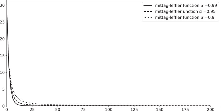
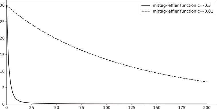
(35) Which is in harmony with a real evolution of an infected isolated population, see Figs. 1 and 2 . From those figures we can remark that number of infected individuals decreases gradually and tends to 0 when t tends to infinity, also from the first figure the fractional order derivative has an effect on the evolution of the epidemic: where α decreases the total number of infected individuals takes more time to vanish, in history the isolation of infected individuals is an old method that had been adopted to prevent the spread of infections, and Public health laws may authorize it in some particular cases.
Fig. 1.
Mittag-Liffler function for I(t) with isolated population such that and 0.95 and 0.9.
Fig. 2.
Mittag-Leffler function for I(t) with isolated population such that and and .
6.2. Euler method
We recall the fractional Euler method [32]. We consider the fractional problem
| (36) |
Then, applying the fractional integral operator to the initial value problem (36), one can obtain
| (37) |
The aim is to approximate the quantity in each point .
With the Explicit Euler Method [32], the quantity
| (38) |
is approximated by
| (39) |
Then,
| (40) |
where
| (41) |
7. Numerical results
In this section, we carry out some numerical results with forward Euler method and variational iteration method for the fractional order SIS model (19) by using different values for the epidemiological parameters b, β and γ. In our case, we use .
We consider the fractional problem (19). If we apply fractional VIM method so, the successive approximations In(t) of the solution I(t) could be manually obtained. Consequently, the solution is given by Eq. (20).
In hand manipulation, one can not easily calculate beyond the third term which is given by formula (32). I 3(t) is a polynomial of degree also we can see that all solutions In(t) are polynomials. With python software, the fractional VIM method can be programmed with the function Vimfrac(b, c, d, alpha, n) which permits to return the polynomial solution for which is of degree . We mention that, this numerical solution becomes effective for long time intervals.
The effect of fractional derivative order on numerical solutions, following variational iteration method and Euler method, is illustrated by the figures below with different values of model parameters.
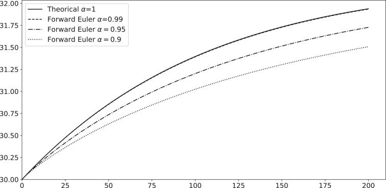
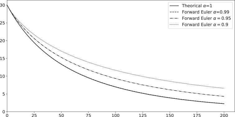
In Figs. 3 and 5 we present the numerical solutions of our fractional model for some values of α near to 1, then we choose for example and we can see that the numerical solution’s trajectory is approaching to the ordinary solution as where as when α is approaching to 1, this numerical analysis is often used in different papers see [4], [7], [9], [12] and [13], we conclude that the fractional model generalizes the ordinary one (19), furthermore, from the same figures, we remark that if the fractional derivative order decreases, the disease takes more time to be eradicated (presence of memory effect).
Fig. 3.
Plots numerical solutions for I(t) such that N=1000, c=0.01, b=0.2, I(0)=30, β=0.31 and 0.95 and 0.9.
Fig. 5.
Plots numerical solutions for I(t) such that N=1000, c=-0.01, b=0.2, I(0)=30, β=0.29 and 0.95 and 0.9.
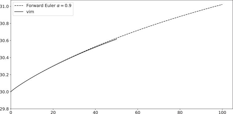
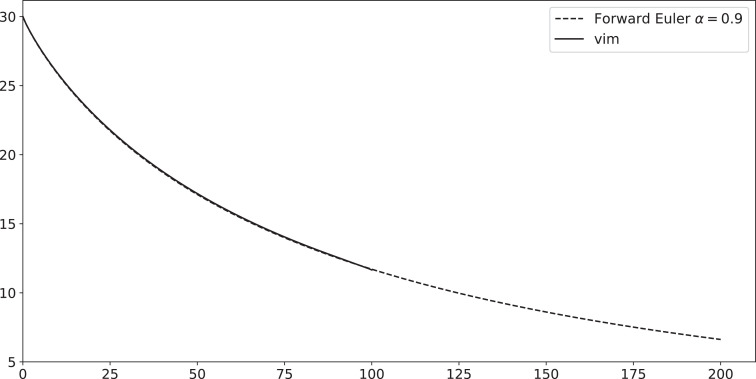
In Figs. 4 and 6 we compare the numerical solution with forward Euler method and variational iteration method, the polynomial used to approximate the solution in Fig. 6 is the vim polynomial of degree 37α, where the polynomial using in Fig. 4 is the vim polynomial of degree 3α. The theoretical VIM method produces a section of symbolic terms of analytical solution, that are hardly to be calculated manually beyond first terms, which makes this method only effective for small time intervals, by the programmed function Vimfrac(b, c, d, alpha, n) we have avoided this restriction, by comparing Figs. 4 and 6, one can remarks the following: the numerical solution is more effective as n increases (In(t)).
Fig. 4.
Plots numerical solutions for I(t) such that N=1000, c=0.01, b=0.2, I(0)=30, β=0.31 and .
Fig. 6.
Plots numerical solutions for I(t) such that N=1000, c=-0.01, b=0.2, I(0)=30, β=0.29 and .
8. Conclusion
The memory is an effect that plays an important role in the evolution of every process related to human societies and the spread of an epidemic is not an exception.
In this paper, we have studied the fractional epidemic SIS model in long time period. We have established the existence and the uniqueness of solution of the fractional system. In order to derive numerical solutions, we have used different methods: the forward Euler method and a recent analytic method for solving nonlinear problem which is variational iteration method (VIM). This method is generally effective only for small time intervals. However, using programming tools, this method becomes efficient to produce numerical results on a long time interval. In our model, some assumptions are taken in order to transform the system to one fractional differential equation for which the ordinary exact solution is calculated formally.
In this perspective, we notice that this fractional model generalizes the ordinary model by comparing the fractional VIM solution and the ordinary exact solution. Finally, the memory effect of the fractional order derivative affects the dynamic of the system, it is noticed from the numerical results that when the value of α is decreased, the disease takes more time to be eradicated and it reflects the memory effect. We strongly believe that this particular SIS model generalizes the ordinary model. Comparing the numerical results and the exact solutions of the ordinary model, the obtained studies can arise some new questions about the specific relations between the fractional order α and the history of biological parameters of the model.
Our analysis has been restricted to a simple local temporal dynamic process in which all epidemiological parameters are supposed to be constant, however, in the field of epidemiology different factors may affect the process of the system like policy, migration and vaccination, taking into account the non locality of geographical spread, is more reasonable to take into consideration special effects in the study of some specific epidemics that cannot supposed to be local like the Black Death in Europe [33], for other mathematical studies on geo-temporal diffusion of epidemics see [34] and [35]. In other context in the classical spread rules of infections the population is divided into a finite number of compartments and infections are controlled by the mass-action law (), in other words we suppose that each individual has the same probability to contact another one in the population, however, in a more realistic study, social relations and families sizes are not identical in the society, so the numbers of contacts differ from a susceptible individual to another, that gives rise to another possible study by modeling the epidemic as network with nods and edges, where nods represent individuals and edges represent a possible contact between two nods this complex study is proposed by Diekmann et al. [36].
Finally, the comprehensive study of basic epidemiological models is essential, our model is a elementary model that could be generalized to a geo-temporal epidemic model or network one, we want also emphasize on the possible extension of our mathematical epidemiological study on analogous models like spreading of rumors, opinions and computer virus.
References
- 1.Saeedian M., Khalighi M., Azimi-Tafreshi N., Jafari G.R., Ausloos M. Memory effects on epidemic evolution: the susceptible-infected-recovered epidemic model. Phys Rev. 2017;95(2):022409. doi: 10.1103/PhysRevE.95.022409. [DOI] [PMC free article] [PubMed] [Google Scholar]
- 2.Hethcote H.W. The mathematics of infectious diseases. SIAM Rev. 2000;42(4):599–653. [Google Scholar]
- 3.Driessche P.V.D., Watmough J. A simple SIS epidemic model with a backward bifurcation. J Math Biol. 2000;40(6) doi: 10.1007/s002850000032. [DOI] [PubMed] [Google Scholar]; 525-40.
- 4.El-Saka H.A.A. Backward bifurcation in fractional-order vaccination models. J Egy Math Soc. 2015;23(1):49–55. [Google Scholar]
- 5.El-Saka H.A.A. The fractional-order SIS epidemic model with variable population. J Egy Math Soc. 2014;22 [Google Scholar]; 50-4.
- 6.Al-Darabsah I., Yuan Y. A time-delayed epidemic model for ebola disease transmission. Appl Math Comput. 2016;290 [Google Scholar]; 307-25.
- 7.Ameen I., Novati P. The solution of fractional order epidemic model by implicit adams methods. Appl Math Model. 2017;43:78–84. [Google Scholar]
- 8.Okyere E., Oduro F.T., Amponsah S.K., Dontwi I.K., Frempong N.K. Fractional order SIR model with constant population. BJMCS. 2016;14(2):1–12. [Google Scholar]
- 9.Banerjee S.K. Analysis of fractional order SIS epidemic model with constant recruitment rate and variable population size. ASIO-JCPMAS. 2016;1(2):01–04. [Google Scholar]
- 10.Sun G.Q., Xie J.H., Huang S.H., Jin Z., Li M.T., Liu L. Transmission dynamics of cholera: mathematical modeling ad control strategies. Commun Nolinear Sci Numer Simulat. 2017;45 [Google Scholar]; 235-44.
- 11.Li L., Wang C.H., Wang S.F., Li M.T., Yakob L., Cazelles B. Hemorrhagic fever with renal syndrome in china: mechanisms on two distinct annual peaks and control measures. Int J Biomath. 2018;11(2):1850030. [Google Scholar]
- 12.Ahmed E.M., El-SAKA H.A. On a fractional order study of middle east respiratory syndrome corona virus (MERS-COV) J Fract Calculus Appl. 2017;8(1) [Google Scholar]; 118-26.
- 13.Singh J., Kumar D., Hammouch Z., Atangana A. A fractional epidemiological model for computer viruses pertaining to a new fractional derivative. Appl Math Comput. 2018;316 [Google Scholar]; 504-15.
- 14.Biazar J. Solution of the epidemic model by adomian decomposition method. Appl Math Comput. 2006;173(2) [Google Scholar]; 1101-6.
- 15.Rafei M., Ganji D.D., Daniali H. Variational iteration method for solving the epidemic model and the prey and predator problem. Appl Math Comput. 2007;186 [Google Scholar]; 1701-9.
- 16.Rafei M., Ganji D.D., Daniali H. Solution of the epidemic model by homotopy perturbation method. Appl Math Comput. 2007;187 [Google Scholar]; 1056-62.
- 17.Awawdeh F., Adawi A., Mustafa Z. Solutions of the SIR models of epidemics using HAM. Chaos Solitons Fractals. 2009;42(5) [Google Scholar]; 3047-52.
- 18.Arqub O.A., El-Ajou A. Solutions of the fractional epidemics model by homotopy analysis method. J King Saud Univ-Sci. 2013;25(1):73–81. [Google Scholar]
- 19.Ahmed E., El-Sayed A.M.A., El-Saka H.A.A. Equilibrium points, stability and numerical solutions of fractional-order predator-prey and rabies models. J Math Anal Appl. 2007;325 [Google Scholar]; 542-53.
- 20.Area I., Batarfi H., Losada J., Nieto J.J., Shammakh W., Torres A. On a fractional order ebola epidemic model. Adv Diff Eq. 2015:278. [Google Scholar]
- 21.Ahmed E., El-Saka H.A. On fractional order models for hepatitis c. Nonlinear Biomed Phys. 2010;4:01–03. doi: 10.1186/1753-4631-4-1. [DOI] [PMC free article] [PubMed] [Google Scholar]
- 22.Pinto C.M.A., Machodo J.A.T. Fractional model for malaria transmission under control strategies. Comp Math Appl. 2013;66(5) [Google Scholar]; 908-16.
- 23.Ye H., Ding Y. Nonlinear dynamics and chaos in fractional-order HIV model. Math Prob Eng. 2009 [Google Scholar]
- 24.Podlubny I. 1th ed. Academic Press; New York: 1999. Fractional differential equations. [Google Scholar]
- 25.Oldham K.B., Spanier J. Acad Press; 1974. The fractional calculus. [Google Scholar]
- 26.Miller K.B., Ross B. John Wiley and Sons Inc; New York: 1993. An introduction to the fractional calculus and fractional differential equations. [Google Scholar]
- 27.Kilbas A.A., Srivastaya H.M., Trujillo J.J. 1th ed. Elsevier; 2006. Theory and applications of fractional differential equations. north-Holland mathematics studies. [Google Scholar]
- 28.Brauer F., Driessche P.V.D., Wu J. Springer; 2008. Mathematical epidemiology, lectures notes in mathematics. [Google Scholar]
- 29.Diethelm K., Ford N.J. The analysis of fractional differential equations. J Math Anal Appl. 2002;265 [Google Scholar]; 229-48.
- 30.He J.H. Variational iteration method - a kind of non-linear analytical technique: some examples. Intern J Non linear Mech. 1999;34:699–708. [Google Scholar]
- 31.Javari H., Tajadodi H. He’S variational iteration method for solving fractional riccati differential equation. Intern J Dif Eq. 2010:764738. [Google Scholar]
- 32.Odibat Z., Moamni S. An algorithm for the numerical solution of differential equations of fractional order. J Appl Math Inform. 2008;26:15–27. [Google Scholar]
- 33.Noble J.V. Geographic and temporal development of plagues. Nature. 1974;250 doi: 10.1038/250726a0. [DOI] [PubMed] [Google Scholar]; 726-9.
- 34.Wang Y., Ma J., Cao J., Li L. Edge-based epidemic spreading in degree-correlated complex networks. J Theor Biol. 2018;454 doi: 10.1016/j.jtbi.2018.06.006. [DOI] [PubMed] [Google Scholar]; 164-81.
- 35.Sun G.Q., Jusup M., Jin Z., Wang Y., Wang Z. Pattern transitions in spatial epidemics: mechanisms and emergent properties. Phys Life Rev. 2016;19:43–73. doi: 10.1016/j.plrev.2016.08.002. [DOI] [PMC free article] [PubMed] [Google Scholar]
- 36.Diekmann O., De Jong M.C.M., Metz J.A.J. A deterministic epidemic model taking account of repeated contacts between the same individuals. J Appl Prob. 1998;35 [Google Scholar]; 448-62.


