

Abstract
A number of Asian cities decided to establish gaming and resort facilities in order to capitalize on the growing number of gamblers and their family members in Asia. In doing so, they expect to sustain economic growth but, on the other hand, will consume a considerable amount of energy. Nevertheless, the causal relationship between economic growth and electricity consumption in this type of service-oriented territories has never been investigated. Using the historical data obtained from the Government of Macao SAR, we found that electricity consumption and economic growth in terms of gross domestic product are co-integrated for the period of 1999 Quarter 1–2008 Quarter 4. Moreover, vector error correction (VEC) models indicated a lack of short-run relationships but showed that there was a long-run equilibrium relationship between electricity consumption and gross domestic product. The accuracy of VEC models was assessed by using the mean squared error and the mean absolute error. The error analysis shows that VEC models reproduced time series of gross domestic product and electricity consumption in difference form accurately.
Keywords: Electricity consumption, Economic growth, Vector error correction model
Research highlights
► Find causal relationship between economic growth and electricity consumption in Macau SAR, PRC – a gaming and tourism center in Asia. ► Indicate long-run and long/short-run relationships from economic growth to electricity consumption in Macau SAR, PRC by Vector Error Correction models. ► Understand about the impacts of gaming and tourism industries to their economic growth and energy consumption. ► Provide a reference to other governments for developments of some gaming and tourism industries in their cities/countries and ► Provide some useful information and suggestions to governmental policy makers in developments of economic growth and energy used.
1. Introduction
Macao, a special administrative region in the People’s Republic of China, has experienced a phenomenal economic growth since the liberalization of the gaming industry in 2002. According to the statistics provided by the Gaming Inspection and Coordination Bureau of Macao, gross revenue from Macao’s casinos amounted to US$13.6 billion in 2008, representing an increase of 31% on year-to-year basis [1]. This figure exceeded the gross income of US$6.12 billion from Las Vegas Strip’s casinos as reported by the Nevada Gaming Commission by a very wide margin. The direct taxes from gaming amounted to US$4.9 billion in 2008, representing 77% of the total income of the Government of Macao SAR. Besides, the annualized gross domestic product (GDP) per capita in Macao was estimated as US$39,036 at the end of 2008, higher than that of Hong Kong and Singapore. As the majority of Macao GDP (62.25%) depends on the gaming and the associated hospitality services provided to visitors, the change in GDP is a good proxy for economic growth in Macao – the world gaming center. In fact, many Asian cities including Singapore and Penghu of Taiwan have decided or proposed to jump on the bandwagon. However, this type of service industry, like the manufacturing sector, consumes a substantial amount of electricity to operate and brighten its infrastructure such as casinos, hotels, resorts, and meeting, exhibition and convention venues day and night. To cope with the increasing demand of electricity consumption, public policy makers in those cities need to have a better understanding on the relationships between economic activities, electricity consumption, and economic growth.
The purposes of this paper are, therefore, (i) to describe the relationship between economic activities and electricity consumption, and (ii) to investigate the long-run relationship and short-run causality relationship between electricity consumption and economic growth in terms of GDP in Macao. The paper is organized as follows. In the next section, we review previous studies on modeling of electricity consumption and literature on causality studies of energy consumption and economic growth. In Section 3, the methodology adopted in the study is presented. Section 4 describes the data employed and reports the findings. Concluding remarks and policy implications are given in Section 5.
2. Literature review on modeling of electricity consumption and the causal relationship between energy consumption and economic growth
Numerous studies have been conducted to examine the relationship between electricity consumption and various economic indicators in the past fifty years. In the 1950s, Houthakker [2] analyzed electricity demand on domestic two-part tariffs for 42 provincial towns in the U.K. He found that average annual electricity consumption per consumer was a function of the average income per household, marginal price of elasticity and marginal price of competing forms of energy, such as gas. Houthakker also reported that the monthly electricity consumption of families had a strong seasonal variation, depending on average temperature and average hours of daylight per day for each month. Foss [3] studied the utilization of capital equipment and suggested that electricity consumption was an indicator of capital usage, especially in an industrial country such as the USA. Foss’s idea was adopted by Jorgensen and Griliches [4] and Heathfield [5] to measure capital usage using electricity consumption data. Mount et al. [6] analyzed both the short-run and long-run demand for electricity for three classes of consumers, namely residential, commercial and industrial. They demonstrated that long-run electricity demand was generally price elastic and became increasingly elastic as prices rose. In contrast, demand was general inelastic with respect to income, especially for residential and industrial classes that approached zero as income increased. Population exhibited approximately unit elasticity for all classes implying the common practice of estimating demand models on a per capita basis to be reasonable. In the past decade, researchers [7], [8], [9], [10], [11], [12] studied the modeling of electricity consumption in different countries or cities. When annual data were used, researchers [8], [10] found that gross national product (GNP) or its derivative such as the number of tourists in a tourist center was the major determinant of electricity consumption. When monthly data were used, researchers found that population (POP), temperature (TEMP) and other economic or industrial factors are the major determinants of electricity consumption [7], [9], [11], [12]. Moreover, Pao [11] reported that economic indicators such as gross domestic product (GDP) and consumer price index (CPI) have a very weak instantaneous effect on Taiwan’s electricity consumption. Lai et al. [12] used multiple regression, artificial neural work (ANN), and wavelet-ANN to model electricity consumption in Macao for the period of January 2000–December 2006. The results show that the total monthly electricity consumption depends on economic factors such as the number of visitors and their hotel-room occupancy rate, demographic and climatic conditions in Macao. Most of the more recent studies show electricity consumption to be strongly associated with the business activities of a country or city.
In pioneering the study of causal relationship between energy consumption and economic growth, Kraft and Kraft [13] used annual data on gross energy inputs and GNP between 1947 and 1974 in the USA and utilized the test for unidirectional causality as outlined by Sims [14]. They found the evidence of a unidirectional causality running from GNP to energy consumption. Yu and Hwang [15] reexamined the causality between energy consumption and GNP over the time period of 1947–1979 using annual data. However, they did not find any evidence to support any causality between energy consumption and GNP over the entire sample period. When the time period was changed to 1973–1981 and quarterly data were used, Yu and Hwang [15] reported that unidirectional causality ran from GNP to energy consumption. A year later, Yu and Choi [16] studied the causal relationship between energy consumption and GNP using Sims and Granger causality tests for five countries. They reported that there was (i) no causal relationship between energy consumption and GNP in the USA, UK and Poland; (ii) unidirectional causality from GNP to energy consumption in South Korea; and (iii) unidirectional causality from energy consumption to GNP in the Philippines. Nachane et al. [17] used Engle–Granger co-integration approach [18] to test the energy–GDP relationship over the time period 1950–51 to 1984–85 for 16 countries. They reported that there was long-run relationship between energy consumption and GDP for 11 developing countries and 5 developed countries. Since then, many researchers [19], [20], [21], [22], [23], [24], [25], [26], [27], [28], [29], [30], [31], [32], [33], [34] adopted Engle–Granger co-integration approach or its modified version to study the causal relationship between energy consumption or electricity consumption and economic growth such as GDP or GNP. Table 1 summarizes the empirical findings of the causality tests between energy consumption and economic growth over the past three decades. The results from more recent studies [23], [24], [25], [26], [27], [28], [29], [30], [31], [32], [33], [34] showed that there was in general a relationship between energy consumption and economic growth. More specifically, Chontanawat et al. [32] suggested that causality from energy to GDP was found to be more prevalent in the Organization for Economic Cooperation and Development (OECD) countries compared to the developing non-OECD countries. However, when it comes to whether the increase in energy consumption is a result of or a cause of economic growth, there is no conclusive agreement on this issue, possibly due to other exogenous factors that may affect energy consumption and GDP simultaneously or sequentially (but have been ignored in most prior studies). Therefore, our study was aimed at studying the relationship between electricity consumption and GDP with the number of tourists and population as important exogenous factors in the world’s gaming center – Macao SAR using Johansen’s methodology [35].
Table 1.
Empirical study on causality between energy consumption and economic growth.
| Authors (Year) | Country | Time period | Methodologies | Findings |
|---|---|---|---|---|
| Kraft and Kraft (1978) [13] | USA | 1947–1974 annual data | Sims’ approach | GNP → energy consumption |
| Yu and Hwang (1984) [15] | USA | i. 1947–1979 annual data | Sims’ approach | GNP [] energy consumption |
| ii. 1973–1981 quarterly data | GNP → energy consumption | |||
| Yu and Choi (1985) [16] | USA | 1963–1976 annual data | Sims and Granger causality tests | GNP [] energy consumption |
| UK | GNP [] energy consumption | |||
| Poland | GNP [] energy consumption | |||
| South Korea | GNP → energy consumption | |||
| Philippines | GNP ← energy consumption | |||
| Nachane et al. (1988) [17] | 16 countries | 1951–1985 annual data | Co-integration and Granger causality tests | |
| Cheng (1995) [19] | USA | 1947–1990 annual data | Hsiao’s version of the Granger causality | GNP [] energy consumption |
| Masih and Masih (1996) [20] | India | 1955–1990 | Johansen’s multivariate co-integration tests | GNP ← energy consumption |
| Pakistan | 1955–1990 | GNP ←→ energy consumption | ||
| Malaysia | 1960–1990 | GNP [] energy consumption | ||
| Singapore | 1955–1990 | GNP [] energy consumption | ||
| Indonesia | 1960–1990 | GNP → energy consumption | ||
| Philippines | 1955–1991 annual data | GNP [] energy consumption | ||
| Cheng and Lai (1997) [21] | Taiwan | 1955–1993 annual data | Co-integration and Hsiao’s version of the Granger causality tests | GDP → energy consumption |
| Glasure and Lee (1998) [22] | South Korea | 1961–1990 | Co-integration and Granger causality tests | GDP [] energy consumption |
| Singapore | 1961–1990 annual data | GDP ← energy consumption | ||
| Yang (2000) [23] | Taiwan | 1954–1997 annual data | Granger causality tests | GDP ←→ energy consumption |
| Hondroyiannis et al. (2002) [24] | Greece | 1960–1996 annual data | Johansen’s method and vector error correction model | GDP ←→ energy consumption |
| Ghosh (2002) [25] | India | 1951–1997 annual data | Co-integration and vector autoregression | GDP → electricity consumption |
| Shiu and Lam (2004) [26] | China | 1971–2000 annual data | Error correction model | GDP ← electricity consumption |
| Oh and Lee (2004) [27] | South Korea | 1981–2000 quarterly data | Vector error correction model | GDP → energy consumption |
| Wolde-Rufael (2006) [28] | 17 African countries | 1971–2001 annual data | Toda-Yamamoto approach | GDP [] electricity consumption in Algeria, Congo Rep., Kenya, South Africa, and Sudan |
| GDP → electricity consumption in Cameroon, Ghana, Nigeria, Senegal, Zambia, and Zimbabwe | ||||
| GDP ← electricity consumption in Benin, Congo DR., and Tunisia | ||||
| GDP ←→ electricity consumption in Egypt, Gabon, and Morocco | ||||
| Yoo (2006) [29] | Indonesia | 1971–2002 annual data | Co-integration and Hsiao’s version of the Granger causality tests | GDP → electricity consumption |
| Malaysia | GDP ←→ electricity consumption | |||
| Singapore | GDP ←→ electricity consumption | |||
| Thailand | GDP ← electricity consumption | |||
| Yuan et al. (2007) [30] | China | 1978–2004 annual data | Error correction model | Real GDP ← electricity consumption |
| Lee and Chang (2007) [31] | 22 developed countries & | 1965–2002 | Panel VAR tests | GDP ←→ energy consumption |
| 18 developing countries | 1971–2002 annual data | GDP → energy consumption | ||
| Chontanawata et al. (2008) [32] | 30 OECD countries and 78 non-OECD countries | 1960–2000 | Co-integration and Hsiao’s version of the Granger causality tests | 26 (87%) OECD countries display some form of Granger causality between energy and GDP. |
| 1971–2000 annual data | 51 (65%) non-OECD countries display some form of Granger-causality between energy and GDP. | |||
| Pao (2009) [33] | Taiwan | 1980–2007 quarterly data | Error correction state space model | Real GDP → electricity consumption |
| Warr and Ayres (2010) [34] | United States | 1946–2000 annual data | Co-integration and the Granger causality tests | Exergy → GDPa |
Note: ←, →, ←→ and [] mean “forward causality”, “backward causality”, “bidirectional causality” and “no relationship”, respectively.
Exergy (the amount of energy available for useful work) was used in Warr and Ayres’s study [34].
3. Methodology
3.1. Granger causality
In his 1969 classic paper on causality, Granger [36] stated that a causal model with two variables is expressed as:
| (1) |
| (2) |
where Xt and Yt are stationary time series. He mentioned that when b 0 = c 0 = 0, Eqs. (1), (2) are the expression for a simple causal model. Granger further noticed that
“Whether or not a model involving some group of economic variables can be a simple causal model depends on what one considers to be the speed with which information flows through the economy and also on the sampling period of the data used. It might be true that when quarterly data are used (let alone the annual data), for example, a simple causal model is not sufficient to explain the relationships between the variables, while for monthly data a simple causal model would be all that is required. Thus, some nonsimple causal models may be constructed not because of the basic properties of the economy being studied but because of the data being used. It has been shown elsewhere that a simple causal mechanism can appear to be a feedback mechanism if the sampling period for the data is so long that details of causality cannot be picked out.” (Granger, 1969, p. 427)
Table 1 shows that there were relative few studies on the causal relationship between energy consumption and economic growth employed quarterly data and most of previous studies were all based on annual data. As the increase in GDP and electricity consumption is more pronounced only after Macao was returned to mainland China in 1999, our study decided to use quarterly data because of the number of data points available and its better ability to capture short-term changes.
3.2. Stationarity and co-integration
Standard Granger causality tests have to be conducted on stationary time series. Engle and Granger [18] stated that economic variables themselves may not be stationary and can have infinite variance, however, they can achieve temporarily stationary after differencing d times (where d is 1, 2, … and so on) and the series can be designated as I(d). When two economic variables Xt and Yt are both I(d), it is generally true that the linear combination Zt = Xt − aYt will also be I(d) [or I(d − b), b > 0. When the latter case occurs, a very special constraint operates on the long-run components of the series. And Xt and Yt are called co-integrated. Following this line, we first test the unit roots of Xt and Yt to confirm the stationary properties of each variable. This is achieved by using the Augmented Dickey–Fuller [37] test and the Phillips–Perron [38] test. For the time series Xt, the Augmented Dickey–Fuller (ADF) relationship is expressed as:
| (3) |
where Δ is the difference operator, p is the auto-regressive lag length that has to be large enough to eliminate possible serial correlation in βi and α and ρ are the coefficients of interest. For time series with strong seasonality, such as quarterly GDP, electricity consumption and the number of tourists, we apply seasonal adjustment before taking the logarithmic transformation as suggested by Pao [33].
When these variables are found to be non-stationary, we take the first-difference and then apply the ADF and Phillips–Perron tests again on the differenced data and so on. To test for co-integration, we employ the Johansen’s vector auto-regressive methodology [35].
3.3. Johansen’s vector auto-regressive (VAR) procedure
Intuitively, the Johansen’s VAR procedure is a multivariate version of the univariate Dickey–Fuller test. Considering a structural form VAR of order p, we have
| (4) |
where k is the number of lags, Zt,Zt −1,…,Zt −k are (2 × 1) vectors containing the logarithmic of seasonally adjusted GDP–ELEC pairs, A 0 is an (2 × 2) structural coefficient matrix, A 1,A 2,…,Ak are (2 × 2) lag coefficient matrices, c o is an (2 × 1) vector containing constant terms, ɛt is an (2 × 1) vector of disturbance terms. We can rewrite this structural VAR in error form (Verbeek [39], p. 326) as:
| (5) |
where . The Π matrix represents the adjustment to disequilibrium following an exogenous disturbance. If Π has a reduced rank r < k where r and k denote the rank of Π and the number of variables constituting the long-run relationship respectively, then there exist two k × r matrices α and β, each with rank r, such that Π = αβ′ and β′yt is stationary. r is called the co-integration rank and each column of β is a co-integrating vector. Johansen’s VAR method estimates the Π matrix from an unrestricted VAR and tests whether one can reject the restrictions implied by the reduced rank of Π. There are two common approaches to test the reduced rank of Π, namely the maximum eigenvalue test and the trace test. For the maximum eigenvalue test, the likelihood ratio is determined from:
| (6) |
where T is the maximum time in the time series t. The null hypothesis of r co-integrating vectors is tested against the alternative hypothesis of r + 1 or more co-integrating vectors. Since the co-integration tests are sensitive to the choice of lag length, we use the Schwartz Information Criteria to determine the optimal lag lengths. On the other hands, the likelihood ratio statistic for the trace test is:
| (7) |
where are the estimated 2 − r smallest values and r = 0 and 1. The null hypothesis is that there are at most r co-integrating vectors. The alternative is that there are r or more co-integrating vectors. Again, we use the Schwartz Information Criteria to determine the optimal lag lengths.
3.4. Vector error correction (VEC) model
If two variables are co-integrated, there is causality between these two variables in at least one direction [40]. If co-integration does not exist between variables, standard VAR in difference form is applied [36]. If co-integration exists between variables, Engle and Granger [18] propose that the VEC model can be used to test Granger causality for at least one direction (also see Oxley and Greasley [41]). The general VECM form is presented as follows.
| (8) |
| (9) |
where Xt and Yt represent the seasonally adjusted GDP and ELEC in logarithmic form, (ΔXt, ΔYt) are the differences in variables, and βi & γj and bi & cj capture the short-term relationships respectively. The μt, vt are the serially uncorrelated error terms. The ECTt −1 is derived from the long-run co-integration relationship. The optimum lag lengths p, q, r and s are determined based on Schwartz Information Criteria.
This specification allows us to test for both short-run and long-run causality. For example, electricity consumption does not Granger cause the growth in GDP in the short-run if and only if all the coefficients γj are equal to zero in Eq. (8). On the other hand, the growth in GDP does not Granger cause electricity consumption if and only if all the coefficients bi are equal to zero in Eq. (9). The presence of long-run causality can be established by examining the significance of the coefficient of the error correction term, ECTt −1 in Eqs. (8), (9) using a t-test. Finally, we conduct a joint test of ECTt −1 and the respective interactive terms in Eqs. (8), (9) using joint F-statistics.
However, if the data are I(1) but not co-integrated, VAR can be applied to the data generated by taking the first-order difference of the variables as shown below [36], [41]:
| (10) |
| (11) |
3.5. Accuracy of VEC models
VEC models do not only describe the causal relationships between endogenous variables, they also present the vector error correction form of dependent variables, i.e. gross domestic product and electricity consumption when the variables are co-integrated in the study, as a function of their past values and exogenous variables. The VEC equations can be used to regenerate time series of dependent variables. As suggested by Lai et al. [12], we adopted the mean squared error (MSE) and the mean absolute error (MAE) to evaluate the accuracy of VEC models. The formulation of MSE and MAE is given as follows:
| (12) |
| (13) |
where e is the error defined as the difference between the actual value and the predicted value using the VEC models.
4. Data and the empirical findings
4.1. Data sources and definition of variables
In this study, we focused on determining the causal relationship between gross domestic product (GDP) and electricity consumption (ELEC), and determined to what extent the number of tourists (TOUR) and population (POP) affect the relationship in the world gaming center. As GDP data was only available on a quarterly basis, we obtained the values of ELEC and TOUR based on quarterly data while POP was taken as the number of residents at the end of each quarter. The values of GDP, ELEC, TOUR and POP for the period of 1999 Quarter 1–2008 Quarter 4 were collected from the Principle Statistical Indicators of Macao published by Macao’s Statistics and Census Service.
ELEC was expressed in terms of kilowatt-hour (kWh) while economic output was characterized by GDP in 2002 prices, using GDP deflators. These variables were transformed to logarithmic values, namely LGDP, LELEC, LTOUR and LPOP, and logarithmic seasonally adjusted values, namely LGDPSA, LELECSA and LTOURSA, before tests were performed as suggested by Pao [33] for quarterly data. Fig. 1, Fig. 2 show the plots of LGDP, LGDPSA, LELEC & LELECSA and LTOUR, LTOURSA & LPOP respectively. They show that GDP, ELEC, TOUR and POP grew between 2001 and 2008, especially after the opening of Sands Macao – a mega casino in May 2005. However, there was a substantial drop in TOUR in the 2nd quarter of 2003 because the outbreak of Severe Acute Respiratory Syndrome (SARS) in Asia. Since the aim of the study was to explore the causal relationship between electricity consumption and economic growth, LGDPSA and LELECSA were set as endogenous variables and LTOURSA and LPOP as exogenous variables in causal analysis. As data magnitude might have an effect on the analysis of causal relationship between variables, time series data were processed by logarithmic transformation and tests were repeated using different combinations of endogenous and exogenous variables, namely LGDPSA, LELECSA, LTOURSA and LPOP. The computer software employed in the study was Eviews 6.0.
Fig. 1.
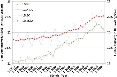
Gross Domestic Product (LGDP) and Electricity Consumption (LELEC) in natural log scale.
Fig. 2.

Tourists and population in natural log scale.
4.2. Results from unit-root tests
Table 2 presents the results of the augmented Dickey–Fuller (ADF) and Philips–Perron (PP) unit-root tests for the two endogenous and two exogenous variables used in the analysis. In each test, we included a constant in the auto-regressive model.
Table 2.
Unit-root tests.
| Variablea | Augmented Dicker–Fuller |
Phillips–Perron |
||
|---|---|---|---|---|
| Lag length | t-Statistics | t-Statistics | ||
| Level | LGDPSA | 0 | −0.223 (<0.93) | −0.178 (<0.93) |
| LELECSA | 0 | −1.551 (<1.00) | −1.779 (<1.00) | |
| LPOP | 1 | −0.382 (<0.98) | −1.954 (<1.00) | |
| LTOURSA | 1 | −0.482 (<0.88) | −0.528 (<0.87) | |
| First-difference | ΔLGDPSA | 0 | −6.496 (<0.01)* | −6.500 (<0.01)* |
| ΔLELECSA | 0 | −6.671 (<0.01)* | −6.638 (<0.01)* | |
| ΔLPOP | 0 | −2.930 (0.05)** | −2.952 (<0.05)** | |
| ΔLTOURSA | 0 | −8.792 (<0.01)* | −10.671 (<0.01)* | |
| Second-difference | Δ2LGDPSA | 0 | −11.454 (<0.01)* | −14.592 (<0.01)* |
| Δ2LELECSA | 0 | −12.441 (<0.01)* | −36.927 (<0.01)* | |
| Δ2LPOP | 0 | −6.687 (<0.01)* | −6.721 (<0.01)* | |
| Δ2LTOURSA | 1 | −8.498 (<0.01)* | −31.021 (<0.01)* | |
Notes: For ADF tests, the optimal lag length was determined using Schwartz Information Criteria. The critical values of the ADF statistic at the 0.01, and 0.05 levels are −4.334, and −3.603 respectively (see MacKinnon [42]). * and ** denote the rejection of the null hypothesis at the 1 percent and 5 percent significance value, respectively and number in parentheses are the corresponding p-values.
Δ and Δ2 denote first-difference and second difference of variables.
According to the ADF results shown in Table 2, the null hypotheses could not be rejected even at the 5 percent level for LGDPSA, LELECSA, LTOURSA, and LPOP in levels but the null hypotheses were rejected at the 1 or 5 percent level for LGDPSA, LELECSA, LPOP and LTOURSA in first and second differences. Therefore, the ADF statistics show that all investigated variables including LGDPSA, LELECSA, LPOP and LTOURSA were integrated of order one, I(1), which are normal for typical economic parameters. Similar conclusions were obtained from the Phillips–Perron (PP) unit-root tests. The null hypotheses were not rejected at the 5 percent level for LGDPSA, LELECSA, LPOP and LTOURSA in levels but were rejected at 1 or 5 percent level for LGDPSA, LELECSA, LPOP and LTOURSA in first and second differences, which indicated an integration order of I(1). The result of this PP unit-root test for all parameters (i.e. I(1)) are the same to that of ADF unit-root test (i.e. I(1)).
4.3. Co-integration analysis
As all variables LGDPSA, LELECSA, LPOP and LTOURSA were non-stationary in levels based on ADF and PP unit-root tests, co-integration test was used to check whether a linear combination of two or more non-stationary series is stationary. The co-integration analysis is typically applied to verify if there exists a long-run relationship between the variables. The results for the Johansen maximum likelihood tests on the unrestricted models are shown in Table 3 .
Table 3.
Johansen and Juselius co-integration tests.
| Variables | Null | Optimal lag | Test statistics |
|
|---|---|---|---|---|
| Trace statistics | Maximum eigenvalue | |||
| LELECSA and LGDPSA#2 | r = 0 | 1 | 22.95* | 19.89* |
| r ≤ 1 | 3.06 | 3.06 | ||
| LELECSA, LGDPSA and LPOP#2 | r = 0 | 1 | 28.98 | 17.61 |
| r ≤ 1 | 11.36 | 7.99 | ||
| r ≤ 2 | 3.37 | 3.37 | ||
| LELECSA, LGDPSA and LTOURSA#2 | r = 0 | 1 | 36.54* | 23.82* |
| r ≤ 1 | 12.72 | 9.03 | ||
| r ≤ 2 | 3.69 | 3.69 | ||
| LELECSA, LGDPSA, LPOP and LTOURSA#2 | r = 0 | 1 | 50.90 | 28.44 |
| r ≤ 1 | 22.46 | 11.44 | ||
| r ≤ 2 | 11.01 | 6.18 | ||
| r ≤ 3 | 4.83 | 4.83 | ||
Notes: The optimal lag lengths are chosen using Schwartz Information Criteria.
* denotes the rejection of the null hypothesis at the 5 percent significance value.
# denotes the co-integration method used as follows: #1. No intercept or trend in co-integrating equation (CE) or VAR, #2. Intercept (no trend) in CE, no intercept or trend in VAR, #3. Intercept in CE and VAR, no trends in CE and VAR, #4. Intercept in CE and VAR, linear trend in CE, no trend in VAR, and #5. Intercept and quadratic trend in the CE and intercept and linear trend in VAR.
Table 3 presents maximum eigenvalues and trace statistics and shows the co-integration relationships among endogenous and exogenous variables. The results of Johansen co-integration tests indicate that LELECSA & LGDPSA & LPOP and LELECSA & LGDP & LPOPSA & LTOURSA did not have co-integration relationships (in Table 3, H0: r = 0, r ≤ 1 and ≤ 2 were accepted at the 5 percent critical level) but LELECSA & LGDPSA and LELECSA & LGDPSA & LTOURSA had one or more than one co-integration equations (in Table 3, H0: r = 0 or r = 0 & r ≤ 1 were rejected at the 5 percent critical level). The optimum lag lengths for different combinations of endogenous and exogenous variables, as shown in Table 3, were determined using the minimum Schwartz Information Criterion (SIC) through unconstrained VAR estimation.
4.4. VEC-based Granger causality test
After having verified the co-integration properties of the variables, vector error correction models were applied to the first-difference variables to determine the long-run and short-run relationships between variables respectively [43], [44], [45]. Based on the previous results of Johansen co-integration tests, two endogenous and exogenous combinations (i.e. LELECSA & LGDPSA and LELECSA & LGDPSA & LTOURSA) were selected for vector error correction (VEC) modeling. However, the combinations with the endogenous variable LPOP did not show co-integration and the major purpose of this analysis is to determine the causality between LELECSA and LGDPSA, the analyses for the combinations with LPOP would not further be conducted. The appropriate lag numbers of different endogenous and exogenous combinations were determined using the minimum Schwartz Information Criterion (SIC). Since the appropriate lag number of these VEC models was 1, we tried different combinations of lag numbers from 1 to 3 in VEC models for comparison.
Three major criteria were adopted to compare various VEC models. They were the goodness of fit, stability and causality. First, the goodness of fit of a VEC model describes how well the regenerated data fit a set of observations as it measures the variability between the actual data and the estimated data using VEC equations. The adjusted coefficient of determination (adjusted R 2) was used to indicate the goodness of fit of the model investigated. The higher adjusted R 2, the better goodness of fit. Moreover, the stability of VEC models is a statistical property of continuance to estimate the stable distributions provided by a linear combination of variables in models. For example, structural changes and/or discontinues in the data typically may cause unstable in estimated models. In VEC models, we applied unit-root tests for determining model stability. Furthermore, t-tests and Wald tests were applied to test whether the long-run relationships and short-run causalities exist in VEC models. In Wald tests, chi-square χ 2 statistics and their probabilities were obtained to determine the short-run causalities in VEC models, respectively. When the probability of chi-square statistics was below 5 percent, the null hypothesis was rejected based on the 5 percent significance level, implying a VEC model having a short-run causal relationship between dependent and independent variables.
Table 4, Table 5 show the VEC findings and the endogeneity of models with the goodness of fit, stability test and causality test, and the final VEC model, respectively. Based on the same three criteria of model selections, all VEC models with endogenous variables ΔLGDPSA & ΔLELECSA passed the stability test but all VEC models with endogenous variables ΔLGDPSA & ΔLELECSA and an exogenous variable ΔLTOURSA failed the stability test. In Wald tests, all VEC models, except ΔLGDPSA equations in VEC models (i.e. ΔLGDPSA & ΔLELECSA and ΔLGDPSA & ΔLELECSA & ΔLTOURSA models) with lag number 3, failed the 5 percent significance level. Moreover, the goodness of fit for the VEC model with endogenous variables ΔLGDPSA & ΔLELECSA, exogenous variables C and lag number 1 was better than that of other models with lag number 1 in average. Moreover, when checking the above-mentioned VEC model, t statistic of exogenous variable ΔLTOURSA(−1) (i.e. ΔLTOURSA with lag number 1) in VEC equations cannot fulfill the t statistics requirement, thus removing ΔLTOURSA(−1). After removing ΔLTOURSA(−1), corresponding adjusted R-squared and stability in the VEC model with endogenous variables ΔLGDPSA & ΔLELECSA, exogenous variable C and lag number 1, were acceptable. Therefore, the VEC model with endogenous variables ΔLGDPSA & ΔLELECSA, exogenous variables C and lag number 1, was found to be the more appropriate one to describe the situation in Macao SAR. On the other hand, we then continued to perform t-test on the error correction term ECT t−1 for long-run causality and joint F test to determine whether short-run adjustment would re-establish long-run equilibrium or not. In Table 7, in VECM equations, the probability of the error correction term ECT t−1 in ΔLGDPSA and ΔLELECSA equations by t-test is 0.6077 and 0.0072 respectively. The results indicated that there was a unidirectional long-run causality from LGDPSA to LELECSA (i.e. LGDPSA → LELECSA in the long-run). Moreover, the joint F test for the sum of lagged terms of each explanatory variable (i.e. ΔLGDPSA and ΔLELECSA) and ECT t−1 term in ΔLGDPSA and ΔLELECSA equations evaluated whether short-run adjustment to re-establish long-run equilibrium, given a shock to the system. The results in Table 6 show that the joint significance of ΔLGDPSA and ECT t−1 term in ΔLELECSA equation existed but that of ΔLELECSA and ECT t−1 term in ΔLGDPSA equation did not exist. This implies that electricity consumption and gross domestic product interact in the short-term to restore long-term equilibrium after a change in gross domestic product. The situation is mainly caused by change in the number of tourists (and their spending behaviors) affecting electricity consumption and gross domestic product at the same time. And after a longer period, the responses in electricity consumption and gross domestic product become stable and restore the equilibrium between electricity consumption and gross domestic product.
Table 4.
Comparison of Vector Error Correction (VEC) model in different lags.
| Endogenous variables | Exogenous variables# | Lag no. | Adjusted R-squared |
Probability in Wald test |
Stability | ||
|---|---|---|---|---|---|---|---|
| Dependent variable |
Dependent variable |
||||||
| ΔLGDPSA | ΔLELECSA | ΔLGDPSA | ΔLELECSA | ||||
| ΔLGDPSA ΔLELECSA | C ΔLTOURSA | 1 | 0.0037 | 0.1195 | 0.7627 | 0.8134 | Unstable |
| ΔLGDPSA ΔLELECSA | C | −0.03206 | 0.1329 | 0.2880 | 0.1653 | Stable | |
| ΔLGDPSA ΔLELECSA | C ΔLTOURSA | 2 | 0.0357 | 0.0555 | 0.1036 | 0.6196 | Unstable |
| ΔLGDPSA ΔLELECSA | C | −0.0049 | 0.0902 | 0.1684 | 0.3010 | Stable | |
| ΔLGDPSA ΔLELECSA | C ΔLTOURSA | 3 | 0.0888 | −0.1146 | 0.0349* | 0.9829 | Unstable |
| ΔLGDPSA ΔLELECSA | C | 0.0617 | −0.0034 | 0.0389* | 0.7320 | Stable | |
Notes: 1. In Wald test, * denotes the rejection of the null hypothesis at the 5 percent significance value. 2. In #, C represents a constant in exogenous variable.
Table 5.
Results of Vector Error Correction (VEC) Model Selected.
| Explanatory variables |
Dependent variable |
|
|---|---|---|
| ΔLGDPSA |
ΔLELECSA |
|
| Co-integrating Eq | CointEq1 | CointEq2 |
| LGDPSA(−1) | 1 | 1 |
| LELECSA(−1) | −1.2085 (0.1431) [−8.4466] | −1.2085 (0.1431) [−8.4466] |
| C in co-integrating Eq | 2.6503 | 2.6503 |
| CointEq | −0.0524 (0.1012) [−0.5182] | 0.1339 (0.0468) [ 2.8610]** |
| ΔLGDPSA(−1) | −0.1483 (0.1956) [−0.7581] | −0.1255 (0.0905) [−1.38739] |
| ΔLELECSA(−1) | 0.3607 (0.3395) [1.0624] | −0.1084 (0.1570) [−0.6901] |
| C | 0.0239 (0.0131) [1.8332] | 0.0265 (0.0060) [4.3802] |
| Adjusted R2 | −0.0321 | 0.1329 |
| F-statistic | 0.61701 | 2.8898 |
| Log likelihood | 51.7299 | 81.0313 |
| Akaike AIC | −2.5121 | −4.0543 |
| Schwarz SC | −2.3397 | −3.8819 |
| Wald test | ||
| Null hypotheses | ΔLELECSA does not Granger cause ΔLGDPSA | ΔLGDPSA does not Granger cause ΔLELECSA |
| Chi-square χ2 statistics | 1.1288 | 1.9249 |
| Degree of freedom | 1 | 1 |
| Probability | 0.2880 | 0.1653 |
Notes: 1. The values in this table are the corresponding coefficient and numbers in parentheses () and brackets [] are the corresponding standard errors and t-values of the parameters, respectively. The parameter symbols of (−1) and (−2) denotes 1 lag value and 2 lag value of their own parameters, respectively.
2. The equivalent equations of ΔLGDPSA and ΔLELECSA are as follows:
ΔLGDPSA = −0.0524*(LGDPSA(−1) − 1.2085*LELECSA(−1) + 2.6502) − 0.1483*ΔLGDPSA(−1) + 0.3607*ΔLELECSA(−1) + 0.0239 ΔLELECSA = 0.1390*(LGDPSA(−1) − 1.2085*LELECSA(−1) + 2.6503) − 0.1255*ΔLGDPSA(−1) − 0.1083*ΔLELECSA(−1) + 0.0264. 3. In Wald test, * denotes the rejection of the null hypothesis at the 5 percent significance value.
4. In VECM, ** denotes the rejection of null hypothesis at the 5 percent significance value in co-integration equations. In VECM equations, the probability of the error correction term in ΔLGDPSA and ΔLELECSA equations by t-test is 0.6077 and 0.0072 respectively. It indicates that there is a long-term causality from LGDPSA to LELECSA (i.e. LGDPSA → LELECSA).
Table 7.
Error analysis of Vector Error Correction (VEC) models.
| Error measures | Dependent variable of VEC |
|
|---|---|---|
| LGDPSA | LELECSA | |
| Mean squared error (MSE) | 0.0038 | 0.0008 |
| Mean absolute error (MAE) | 0.0433 | 0.0224 |
Table 6.
Estimation results of joint test for logarithmic series of seasonally adjusted GDP and electricity consumption.
| Source of causality | ||
|---|---|---|
| Dependent variables | Joint short/long-term test |
|
| ΔGDPSA and ECT | ΔELECSA and ECT | |
| F-statistics | ||
| ΔGDPSA | – | 0.6512 |
| ΔELECSA | 4.1797** | – |
Notes: 1.ΔGDPSA and ΔELECSA are the first-difference series of LGDPSA and LELECSA respectively; ECT is the Error Correction Term. Δ denotes first-difference of variables. 2. * and ** denote the rejection of the null hypothesis at the 1 percent and 5 percent significance value, respectively.
Overall, the ΔLGDPSA & ΔLELECSA VEC models indicated a long-run causality and joint short/long-run causality from gross domestic product to electricity consumption (ΔLGDPSA → ΔLELECSA in the long-run), but no short-run causality existed. They represent that short-run and long-run relationships are different. The ΔLGDPSA equation indicated that there was no short-run, long-run and joint short/long-run causality. The ΔLELECSA equation, however, indicated that there was a long-run (and joint short/long-run) causality but no short-run causality. These results indicated that although no short-run causality from gross domestic product to electricity existed, short-run interaction can lead to a long-run causality. Moreover, the long-run causality from gross domestic product to electricity existed significantly. The VEC model shown in Table 7 is given as follows:
| (14) |
| (15) |
The results of VEC shown in Table 4, Table 5, Table 6 matched with the results of co-integration tests shown in Table 3. Based on these analyses, we conclude that there was a unidirectional long-run relationship from gross domestic product to electricity consumption.
4.5. Error analysis of VEC models
Eqs. (14), (15) were used to regenerate the values of ΔLGDPSA and ΔLELECSA for the period of 1999 Quarter 3–2008 Quarter 4. The regenerated data were then compared to the actual data and the MSE and MAE were determined using Eq. (12), (13). The values of MSE and MAE were 0.0038 and 0.0433 for ΔLGDPSA and 0.0008 and 0.0224 for ΔLELECSA respectively, as shown in Table 7. One-sample t-tests show that the values of squared error and the values of absolute error of ΔLDGPSA and ΔLELECSA were not significantly different from zero at the 95 percent level of confidence. The results illustrate that VEC models reproduced time series of ΔLGDPSA and ΔLELECSA accurately.
5. Concluding remarks and implications
Co-integration analyses show that there was a co-integrated relationship between seasonally adjusted electricity consumption and economic growth (LELECSA and LGDPSA) in Macao over the period of 1999 Quarter 1–2008 Quarter 4. Vector error correction models indicated that there was a long-run unidirectional causal relationship from gross domestic product to electricity consumption. Moreover, given a change in gross domestic product, gross domestic product and electricity consumption interacted in short-term and then re-established the long-run equilibrium. Co-integration test showed that seasonally adjusted gross domestic product, electricity and tourists’ amount in natural log scale (LGDPSA, LELECSA and LTOURSA) were co-integrated. Although in previous section, we adopted the VEC model with ΔLGDPSA and ΔLELECSA only, change in the number of tourists (ΔTOURSA) will have a peculiar effect on ΔLGDPSA than on ΔLELECSA. It can be understood because the gaming and tourism center in Asia Macao SAR depends heavily on the tourism industry (but in fact more on the high rollers among those tourists). The number of tourists (more specifically, the number of high rollers) affects significantly and positively on gross domestic product and in turn affects electricity consumption. A detailed observation of the ΔLELECSA VEC equation reveals that ΔLELECSA depends heavily and significantly on the lag 1 of ΔLGDPSA. This implies that in a service-oriented territory, infrastructures such as casinos, hotels, resorts, convention centers, food-serving outlets, etc. have to be built (leading to a sudden increase in GDPSA) and operated to attract tourists, consequently leading to a positive change in the city’s or national electricity consumption.
The results provide useful information to policy makers in other Asian cities or countries. First, a city can enjoy the economic growth brought by the development of the gaming and tourism industry but policy makers have to find ways to produce and utilize their electricity more environmentally friendly and efficiently. It is because the depletion of energy resources and the emission of carbon dioxide – a major greenhouse gas are recognized as international problems. Nevertheless, it is possible that operators of entertainment venues can adopt a wide range of energy saving practices, such as adopting variable speed drives for fans, pumps and lifts, introducing heat exchangers and heat pumps in air-conditioning and refrigerating systems, and adopting energy-efficient and yet cost effective and environmental-friendly commercial applicants [46], etc. Second, whether the gaming industry will bring negative impacts on social and cultural systems is debatable [47]. Macao’s economic development in recent years is eye-opening. However, the number of young problem gamblers has increased over time.
Acknowledgment
The authors gratefully acknowledge support of this work by the Macao Polytechnic Institute through Grant P014/DECP/2009. We also thank anonymous reviewers for many valuable comments that improve the paper greatly.
References
- 1.DICJ . Macao Gaming Inspection and Coordination Bureau; 2009. Gaming statistical information of Macao.http://www.dicj.gov.mo/web/cn/information/DadosEstat/2009/content.html#n1 See also: [Google Scholar]
- 2.Houthakker H.S. Some calculations on electricity consumption in Great Britain. J R Stat Soc Ser A – Gen. 1951;114(3):359–371. [Google Scholar]
- 3.Foss MR. The utilization of capital equipment: postwar compared with prewar. Survey of Current Business, Washington D.C., Bureau of Census, 1963:8–16.
- 4.Jorgensen D.W., Griliches Z. The explanation of productivity change. Rev Econ Stud. 1967;34:249–283. [Google Scholar]
- 5.Heathfield D.F. The measurement of capital usage using electricity consumption data for the UK. J R Stat Soc Ser A – Gen. 1972;135(2):208–220. [Google Scholar]
- 6.Mount T.D., Chapman L.D., Tyrrell T.J. Oak Ridge National Laboratory; Oak Ridge, TN: 1973. Electricity demand in the US: an econometric analysis. [Google Scholar]
- 7.Ranjan M., Jain V.K. Modeling of electrical energy consumption in Delhi. Energy. 1999;24:351–361. [Google Scholar]
- 8.Egolioglu F., Mohamad A.A., Guven H. Economic variables and electricity consumption in North Cyprus. Energy. 2001;26:355–362. [Google Scholar]
- 9.Nasr G.E., Badr E.A., Younes M.R. Neural networks in forecasting electrical energy consumption: univariate and multivariate approaches. Int J Energy Res. 2002;26:67–78. [Google Scholar]
- 10.Ozturk H.K., Ceylan H. Forecasting total and industrial sector electricity demand based on genetic algorithm approach: Turkey case study. Int J Energy Res. 2005;29:829–840. [Google Scholar]
- 11.Pao H.T. Comparing linear and nonlinear forecasts for Taiwan’s electricity consumption. Energy. 2006;31:2129–2141. [Google Scholar]
- 12.Lai T.M., To W.M., Lo C.W., Choy Y.S. Modeling of electricity consumption in the Asian gaming and tourism center – Macao SAR, People’s Republic of China. Energy. 2008;33:679–688. [Google Scholar]
- 13.Kraft J., Kraft A. On the relationship between energy and GNP. J Energy Dev. 1978;3:401–403. [Google Scholar]
- 14.Sims C.A. Money, income, and causality. Am Econ Rev. 1972;62(4):540–552. [Google Scholar]
- 15.Yu E.S.H., Hwang B.K. The relationship between energy and GNP: further results. Energy Econ. 1984;6:186–190. [Google Scholar]
- 16.Yu E.S.H., Choi J.Y. The causal relationship between energy and GNP: an international comparison. J Energy Dev. 1985;10:249–272. [Google Scholar]
- 17.Nachane D.M., Nadkarni R.M., Karnik A.V. Co-integration and causality testing of the energy–GDP relationship: a cross-country study. Appl Econ. 1988;20(11):1511–1531. [Google Scholar]
- 18.Engle R.F., Granger C.W.J. Co-integration and error correction: representation, estimation, and testing. Econometrica. 1987;55(2):251–276. [Google Scholar]
- 19.Cheng B.S. An investigation of co-integration and causality between energy consumption and economic growth. J Energy Dev. 1995;21:73–84. [Google Scholar]
- 20.Masih A.M.M., Masih R. Energy consumption, real income and temporal causality: results from a multi-country study based on cointegration and error-correction modeling techniques. Energy Econ. 1996;18:165–183. [Google Scholar]
- 21.Cheng B.S., Lai W.T. An investigation of co-integration and causality between energy consumption and economic activity in Taiwan. Energy Econ. 1997;19:435–444. [Google Scholar]
- 22.Glasure Y.U., Lee A.R. Cointegration, error correction and the relationship between GDP and energy: the case of South Korea and Singapore. Res Energy Econ. 1998;20:17–25. [Google Scholar]
- 23.Yang H.Y. A note on the causal relationship between energy and GDP in Taiwan. Energy Econ. 2000;22(3):309–317. [Google Scholar]
- 24.Hondroyiannis G., Lolos S., Papapetrou E. Energy consumption and economic growth assessing the evidence from Greece. Energy Econ. 2002;24:319–336. [Google Scholar]
- 25.Ghosh S. Electricity consumption and economic growth in India. Energy Policy. 2002;30(2):125–129. [Google Scholar]
- 26.Shiu A., Lam P.L. Electricity consumption and economic growth in China. Energy Policy. 2004;32(1):47–54. [Google Scholar]
- 27.Oh W.K., Lee K.H. Energy consumption and economic growth in Korea: testing the causality relation. J Policy Mod. 2004;26:973–981. [Google Scholar]
- 28.Wolde-Rufael Y. Electricity consumption and economic growth: a time series experience for 17 African countries. Energy Policy. 2006;34(10):1106–1114. [Google Scholar]
- 29.Yoo S.H. The causal relationship between electricity consumption and economic growth in the ASEAN countries. Energy Policy. 2006;34:3573–3582. [Google Scholar]
- 30.Yuan J., Zhao C., Yu S., Hu Z. Electricity consumption and economic growth in China: cointegration and co-feature analysis. Energy Econ. 2007;29:1179–1191. [Google Scholar]
- 31.Lee C.C., Chang C.P. Energy consumption and GDP revisited: a panel analysis of developed and developing countries. Energy Econ. 2007;29:1206–1223. [Google Scholar]
- 32.Chontanawat J., Hunt L.C., Pierse R. Does energy consumption cause economic growth?: Evidence from a systematic study of over 100 countries. J Policy Model. 2008;30(2):209–220. [Google Scholar]
- 33.Pao H.T. Forecast of electricity consumption and economic growth in Taiwan by state space modeling. Energy. 2009;34:1779–1791. [Google Scholar]
- 34.Warr B.S., Ayres R.U. Evidence of causality between the quantity and quality of energy consumption and economic growth. Energy. 2010;35:1688–1693. [Google Scholar]
- 35.Johansen S. Statistical analysis of cointegration vectors. J Econ Dyn Cont. 1988;12:231–254. [Google Scholar]
- 36.Granger C.W. Investigating causal relations by econometric models and cross-spectral methods. Econometrica. 1969;37(3):424–438. [Google Scholar]
- 37.Dickey D.A., Fuller W.A. Distribution of the estimators for autoregressive time series with a unit root. J Am Stat Assoc. 1979;74:427–431. [Google Scholar]
- 38.Phillips P.C.B., Perron P. Testing for a unit root in time series regression. Biometrika. 1988;75:335–346. [Google Scholar]
- 39.Verbeek M. 2nd ed. John Wiley & Sons; Chichester: 2004. A guide to modern econometrics. [Google Scholar]
- 40.Granger C.W.J. Some recent developments in a concept of causality. J Econometrics. 1988;39:199–211. [Google Scholar]
- 41.Oxley L., Greasley D. Vector autoregression, cointegration and causality: testing for causes of the British industrial revolution. Appl Econ. 1998;30:1387–1397. [Google Scholar]
- 42.MacKinnon J.G. Numerical distribution functions for unit root and cointegration tests. J Appl Econometrics. 1996;11(6):601–618. [Google Scholar]
- 43.Toda H.Y., Yamamoto T. Statistical inference in vector autoregressions with possibly integrated process. J Econometrics. 1995;66(1–2):225–250. [Google Scholar]
- 44.Zapata H.O., Rambaldi A.N. Monte Carlo evidence on cointegration and causation. Oxford Bull Econ Stat. 1997;59(2):285–298. [Google Scholar]
- 45.Kanioura A., Turner P. Critical values for an F-test for cointegration in the multivariate model. Appl Econ. 2005;37(3):265–270. [Google Scholar]
- 46.To W.M., Yu T.W., Lai T.M., Li S.P. Characterization of commercial clothes dryers based on energy-efficiency analysis. Int J Clothing Sci Technol. 2007;19(5):277–290. [Google Scholar]
- 47.Kwan F.V.C. Changes in residents’ gambling attitudes and perceived impacts at the fifth anniversary of Macao’s gaming deregulation. J Travel Res. 2009;47(3):388–397. [Google Scholar]