Analysis and control of an SEIR epidemic system with nonlinear transmission rate

Abstract

In this paper, the dynamical behaviors of an SEIR epidemic system governed by differential and algebraic equations with seasonal forcing in transmission rate are studied. The cases of only one varying parameter, two varying parameters and three varying parameters are considered to analyze the dynamical behaviors of the system. For the case of one varying parameter, the periodic, chaotic and hyperchaotic dynamical behaviors are investigated via the bifurcation diagrams, Lyapunov exponent spectrum diagram and Poincare section. For the cases of two and three varying parameters, a Lyapunov diagram is applied. A tracking controller is designed to eliminate the hyperchaotic dynamical behavior of the system, such that the disease gradually disappears. In particular, the stability and bifurcation of the system for the case which is the degree of seasonality ${\beta }_1=0$ are considered. Then taking isolation control, the aim of elimination of the disease can be reached. Finally, numerical simulations are given to illustrate the validity of the proposed results.

1. Introduction

Mathematical models describing the population dynamics of infectious diseases have been playing an important role in a better understanding of epidemiological patterns and disease control for a long time. In order to predict the spread of infectious disease among regions, many epidemic models have been proposed and analyzed in recent years (see [1], [2], [3], [4]). However, most of the literature researched on epidemic systems (see [5], [6], [7], [8]) assumes that the disease incubation is negligible which causes that, once infected, each susceptible individual (in class $S$) becomes infectious instantaneously (in class $I$) and later recovers (in class $R$) with a permanent or temporary acquired immunity. The model based on these assumptions is customarily called an SIR (susceptible-infectious-recovered) or SIRS (susceptible- infectious-recovered-susceptible) system (see [9], [10]). Many diseases such as measles, severe acute respiratory syndromes (SARS) and so on, however, incubate inside the hosts for a period of time before the hosts become infectious. So the systems that are more general than SIR or SIRS types need to be studied to investigate the role of incubation in disease transmission. We may assume that a susceptible individual first goes through a latent period (and said to become exposed or in the class $E$) after infection before becoming infectious. Thus the resulting models are of SEIR (susceptible- exposed-infectious-recovered) or SEIRS (susceptible-exposed-infectious-recovered-susceptible) types, respectively, depending on whether the acquired immunity is permanent or not. Many researchers have studied the stability, bifurcation or chaos behavior of SEIR or SEIRS epidemic systems (see [11], [12], [13], [14], [15], [16]). Michael et al. [11] study the global stability of an SEIR epidemic system in the interior of the feasible region. Greenhalgh [17] discusses Hopf bifurcation in models of SEIRS type with density dependent contact and death rates. In addition, some literature on the SEIR-type age-independent epidemic systems has been investigated by many authors (see [15], [17], [18]) and their threshold theorems are well obtained.

Many authors find that most practical systems are more exactly described by differential and algebraic equations, which appear in engineering systems such as power systems, aerospace engineering, biological systems, economic systems, etc. (see [19], [20], [21], [22]). Although many epidemic systems can be described by differential and algebraic equations (see [2], [13], [16], [23]), they are studied by reducing the dimension of epidemic models to differential systems and the dynamical behaviors of the whole systems are not better described. By reducing the dimension of an SEIR epidemic system via substituted algebraic constraint into differential equations and using the methods of reconstructed phase and correlation dimension, Olsen and Schaffer [13] studied the system described by differential equations that is chaos with a degree of seasonality ${\beta }_1=0.28$. However, we can find more complex dynamical behaviors if the SEIR epidemic system is described by differential and algebraic equations via an analysis of the whole system. The systemic parameters in this paper are same as [13]. In particular, the system is hyperchaotic when systemic parameter ${\beta }_1=0.28$ in this paper. Some authors study biologic systems based on seasonal forcing. Kamo and Sasaki [24] discuss dynamical behaviors of a multi-strain SIR epidemiological model with seasonal forcing in the transmission rate. Broer et al. [25] studied the dynamics of a predator-prey model with seasonal forcing.

Differential and algebraic systems are also referred as descriptor systems, singular systems, generalized state space systems, etc. Differential and algebraic systems are governed by the so-called singular differential equations, which endow the systems with many special features that are not found in classical systems. Among these are impulse terms and input derivatives in the state response, nonproperness of transfer matrix, noncausality between input and state (or output), consistent initial conditions, etc. Research on nonlinear differential and algebraic systems has focused on systems with the following description:

$$\Xi \left(t\right)\dot{x}\left(t\right)=H(x\left(t\right),u\left(t\right),t)$$$$y\left(t\right)=J(x\left(t\right),u\left(t\right),t)$$ (1.1)

where $\Xi \left(t\right)\in {\mathbb{R}}^n\times {\mathbb{R}}^n$ is singular; $H$ and $J$ are appropriate dimensional vector functions in $x\left(t\right)$, $u\left(t\right)$ and $t$; $x\left(t\right)$, $u\left(t\right)$ and $y\left(t\right)$ are the appropriate dimensional state, and input and output vectors, respectively; $t$ is a time variable. In particular, the systems (1.1) are normal systems if $\mathrm{rank}\left[\Xi \left(t\right)\right]=n$. Some authors have discussed chaotic dynamical behavior and chaotic control based on differential and algebraic systems. Zhang et al. [26], [27] discuss chaos and their control of singular biological economy systems by the theory of differential and algebraic systems.

The literature mentioned above is concerned about low-dimensional chaotic systems with one positive Lyapunov exponent. The attractor of chaotic systems that may have two or more positive Lyapunov exponents is called hyperchaos. However, many researchers have investigated hyperchaotic systems which are the classical hyperchaotic systems, such as hyperchaotic Chen systems, hyperchaotic Rossler systems, hyperchaotic Lorenz systems and so on (see [28], [29], [30], [31]). They are all based on hyperchaos synchronization and hyperchaos control. Up to now, a wide variety of approaches have been used to control hyperchaotic systems, for example, the sliding mode control, state feedback control, adaptive control and tracking control, etc. (see [32], [33], [34], [35]). However, no literature discusses hyperchaos and its control based on differential and algebraic systems.

To the best of our knowledge, hyperchaos appears first in differential and algebraic systems based on this paper. The contribution of this paper can be divided into three main parts. In the first part, an SEIR epidemic system with seasonal forcing in transmission rate, which is a new form of differential and algebraic system, is modeled. We discuss the cases of only one varying parameter, two varying parameters and three varying parameters, respectively. For the case of one varying parameter, the periodic, chaotic and hyperchaotic dynamical behaviors of the system are analyzed via the bifurcation diagrams, Lyapunov exponent spectrum diagram and Poincare section. For the cases of two and three varying parameters, the dynamical behaviors of the system are investigated by using Lyapunov diagrams. In the second part, for the hyperchaotic dynamical behavior of the system, we design a tracking controller such that the infectious trajectory of the system tracks an ideal state $i_d\left(t\right)=0$. In the last part, the case for the degree of seasonality ${\beta }_1=0$ is studied. Taking isolation control, we reach the aim of elimination of the disease, and it is easy to implement in real life.

This paper is organized as follows. In Section 2, some preliminaries for the differential and algebraic systems are introduced and the SEIR model is described by differential and algebraic equations. In Section 3, the dynamical behaviors of the model are analyzed and a tracking controller is designed for the hyperchaotic system, such that the infected gradually disappears. In particular, the case for the degree of seasonality ${\beta }_1=0$ is studied. Taking isolation control, the aim of elimination of the disease can be reached. Simulation results are presented to demonstrate the validity of the controller. Some concluding remarks are given in Section 4.

2. Preliminaries and description of the model

In this section, we describe the SEIR epidemic model and introduce some correlative definitions about differential and algebraic systems.

We describe an SEIR epidemic model with nonlinear transmission rate as follows. The population of size $N\left(t\right)$ is divided into classes containing susceptible, exposed (infected but not yet infectious), infectious and recovered. At time $t$, there are $S\left(t\right)$ susceptible, $E\left(t\right)$ exposed, $I\left(t\right)$ infectious, and $R\left(t\right)$ recovered. The host total population is $N\left(t\right)=S\left(t\right)+E\left(t\right)+I\left(t\right)+R\left(t\right)$ at time $t$. And we assume that immunity is permanent and that recovered individuals do not revert to the susceptible class. It is assumed that all newborns are susceptible (no vertical transmission) and a uniform birthrate. The dynamical transfer of the population is depicted in Fig. 1 .

Fig. 1.

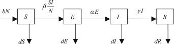
The dynamical transfer of the population $N$.

The parameter $b>0$ is the rate for natural birth and $d>0$ is the rate for natural death. The parameter $\alpha >0$ is the rate at which the exposed individuals become infective, so $1/\alpha$ means the latent period and $\gamma >0$ is the rate for recovery. The force of infection is $\frac{\beta I}{N}$, where $\beta >0$ is effective per capita contact rate of infective individuals and the incidence rate is $\frac{\beta IS}{N}$.

The following differential and algebraic system is derived based on the basic assumptions and using the transfer diagram

$$\dot{S}\left(t\right)=bN\left(t\right)-dS\left(t\right)-\beta \frac{S\left(t\right)I\left(t\right)}{N\left(t\right)}$$$$\dot{E}\left(t\right)=\beta \frac{S\left(t\right)I\left(t\right)}{N\left(t\right)}-(\alpha +d)E\left(t\right)$$$$\dot{I}\left(t\right)=\alpha E\left(t\right)-(\gamma +d)I\left(t\right)$$$$\dot{R}\left(t\right)=\gamma I\left(t\right)-dR\left(t\right)$$$$0=S\left(t\right)+E\left(t\right)+I\left(t\right)+R\left(t\right)-N\left(t\right)\text{.}$$ (2.1)

Remark 1

The system (2.1) is a classical epidemiological one (see [2]) when the population size $N\left(t\right)$ is assumed to be a constant and normalized to 1.

Remark 2

The rate of removal $\alpha$ of individuals from the exposed class is assumed to be a constant so that $1/\alpha$ can be regarded as the mean latent period. In the limiting case, when $\alpha \to \infty$, the latent period $1/\alpha \to 0$, the SEIR model becomes an SIR model (see [24]).

From the first to fourth differential equations of system (2.1) describe the dynamical behaviors of every dynamic element for whole epidemic system (2.1) and the last algebraic equation describes the restriction of every dynamic element of system (2.1). That is, the differential and algebraic system (2.1) can describe the whole behavior of certain epidemic spreads in a certain area.

We consider the transmission rate with seasonal forcing in this paper as follows:

$$\beta ={\beta }_0(1+{\beta }_{1}cos2\pi t)$$

where ${\beta }_0$ is the base transmission rate, and ${\beta }_1(0\le {\beta }_1\le 1)$ measures the degree of seasonality.

We make the transformation

$$s=\frac{S}{N}\text{,}e=\frac{E}{N}\text{,}i=\frac{I}{N}\text{and}r=\frac{R}{N}$$

to obtain the following differential and algebraic system:

$$s^{\prime }=b-bs-\beta si$$$$e^{\prime }=\beta si-(\alpha +b)e$$$$i^{\prime }=\alpha e-(\gamma +b)i$$$$r^{\prime }=\gamma i-br$$$$0=s+e+i+r-1$$ (2.2)

where $s$, $e$, $i$, $r$ denote the proportions of susceptible, exposed, infectious and recovered, respectively. Note that the total population size $N$ does not appear in system (2.2), this is a direct result of the homogeneity of the system (2.1). Also observe that the variable $r$ is described by differential equation $r^{\prime }=\gamma i-br$ as well as algebraic equation $r=1-s-e-i$, but there is no the variable $r$ in the first to third equations of the system (2.2). This allows us to attack system (2.2) by studying the subsystem

$$s^{\prime }=b-bs-\beta si$$$$e^{\prime }=\beta si-(\alpha +b)e$$$$i^{\prime }=\alpha e-(\gamma +b)i$$$$0=s+e+i+r-1\text{.}$$ (2.3)

System (2.3) is also a differential and algebraic system. The dynamical transfer of the epidemic model such as measles, smallpox, chicken-pox etc. accords with the description of system (2.3).

From biological considerations, we study system (2.3) in the closed set:

$$\Gamma =\{(s,e,i,r)\in {\mathbb{R}}_{+}^4|s+e+i+r=1\}\text{,}$$

where ${\mathbb{R}}_{+}^4$ denotes the non-negative cone of ${\mathbb{R}}^4$.

We introduce some definitions that are used in this paper as follows.

We consider the following differential and algebraic system [22]:

$$\dot{X}\left(t\right)=f(X\left(t\right),Y\left(t\right))+g(X\left(t\right),Y\left(t\right))u\left(t\right)$$$$0=p(X\left(t\right),Y\left(t\right))$$ (2.4)

where $X\left(t\right)={(X_1\left(t\right),X_2\left(t\right),\dots ,X_n\left(t\right))}^T,Y\left(t\right)={(Y_1\left(t\right),Y_2\left(t\right),\dots ,Y_m\left(t\right))}^T$ and $u\in \mathbb{R}$ are the $n$ dimensional state variable, $m$ dimensional constraint variable and control input, respectively. $f:{\mathbb{R}}^n\times {\mathbb{R}}^m\to {\mathbb{R}}^n$; $g:{\mathbb{R}}^n\times {\mathbb{R}}^m\to {\mathbb{R}}^n$ and $p:{\mathbb{R}}^n\times {\mathbb{R}}^m\to {\mathbb{R}}^n$ are smooth vector fields, and

$$\mathrm{rank}\left(\frac{\partial p(X,Y)}{\partial Y}\right)=m\text{,}\forall (X\left(t\right),Y\left(t\right))\in \Omega \subset {\mathbb{R}}^n\times {\mathbb{R}}^m\text{,}$$

$\Omega$ is an open connectible set.

Definition 1 $M$ derivative [36] —

$M_f\left(q(X\left(t\right),Y\left(t\right))\right)$ and $M_g\left(q(X\left(t\right),Y\left(t\right))\right)$ are said to be the derivatives of $M$ about vector fields $f$ and $g$ at the function $q(X\left(t\right),Y\left(t\right))$, respectively, if the following equations

$$M_f\left(q(X\left(t\right),Y\left(t\right))\right)=\phi \left(q(X\left(t\right),Y\left(t\right))\right)f\text{and}$$

$$M_g\left(q(X\left(t\right),Y\left(t\right))\right)=\phi \left(q(X\left(t\right),Y\left(t\right))\right)g\text{,}$$

hold, where

$$\varphi \left(q(X\left(t\right),Y\left(t\right))\right)=\frac{\partial q}{\partial X\left(t\right)}-\frac{\partial q}{\partial Y\left(t\right)}{\left(\frac{\partial p}{\partial Y\left(t\right)}\right)}^{-1}\frac{\partial p}{\partial X\left(t\right)}\text{.}$$

Definition 2 Relative degree [36] —

Assume that the output function of system (2.4) is $h(X\left(t\right),Y\left(t\right))$, when $(X\left(t\right),Y\left(t\right))\in \Omega \subset {\mathbb{R}}^n\times {\mathbb{R}}^m$, there exists a positive integer $\theta$ which is called the relative degree if the following conditions are satisfied:

$$M_g{M}_f^{k}h(X\left(t\right),Y\left(t\right))\equiv 0\text{,}k=0,\dots ,\theta -2\text{;}$$

$$M_g{M}_f^{\theta -1}h(X\left(t\right),Y\left(t\right))\ne 0\text{.}$$

3. Main results

3.1. Analysis of dynamical behaviors

In this subsection, we not only consider the case of only one varying parameter ${\beta }_1$, but also discuss the cases of two and three varying parameters. For the case of only one varying parameter ${\beta }_1$, the dynamical behaviors of system (2.3) are analyzed by using the bifurcation diagrams, Lyapunov exponent spectrum diagram and Poincare section. In particular, there is hyperchaotic dynamical behavior for system (2.3) with ${\beta }_1=0.28$, i.e., system (2.3) has two positive Lyapunov exponents. For the cases of two and three varying parameters, the dynamical behaviors of system (2.3) are analyzed by using Lyapunov diagrams.

3.1.1. Only one varying parameter

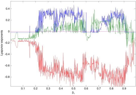
Let ${\beta }_1$ be a varying parameter of system (2.3), and the rest of the parameters are $b=0.02$, $\alpha =35.84$, $\gamma =100$ and ${\beta }_0=1800$, respectively (see [13]). The bifurcation diagrams of systemic parameter ${\beta }_1$ and every variable of system (2.3) using Matlab7.1 software are shown in Fig. 2 . From Figs. 2. (a), (b), (c) and (d), we can easily see that there are complicated dynamical behaviors for system (2.3) with parameter ${\beta }_1$ in some areas. The corresponding Lyapunov exponent spectrum diagram is given in Fig. 3a, Fig. 3b, Fig. 3c . Figs. 2, and Fig. 3a, Fig. 3b, Fig. 3c show how the dynamics of system (2.3) change with the increasing value of the parameter ${\beta }_1$. We can observe that the Lyapunov exponent spectrum gives results completely consistent with the bifurcation diagram. In particular, Fig. 3c shows that there are two positive Lyapunov exponents with the parameter ${\beta }_1=0.28$, i.e., system (2.3) with ${\beta }_1=0.28$ is hyperchaotic.

Fig. 2.

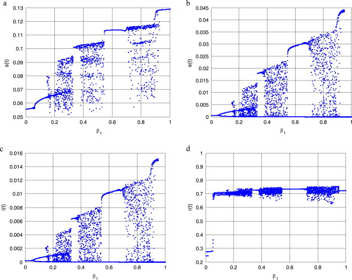
Bifurcation diagrams of parameter ${\beta }_1(0\le {\beta }_1\le 1)$ and every variable of system (2.3). (a) ${\beta }_1-s\left(t\right)$; (b) ${\beta }_1-e\left(t\right)$; (c) ${\beta }_1-i\left(t\right)$; (d) ${\beta }_1-r\left(t\right)$.

Fig. 3a.

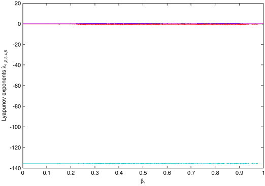
Corresponding Lyapunov exponents of system (2.3) versus parameter ${\beta }_1$.

Fig. 3b.

Local amplification of Fig. 3a for Lyapunov exponent values in (−1, 0.5).

Fig. 3c.

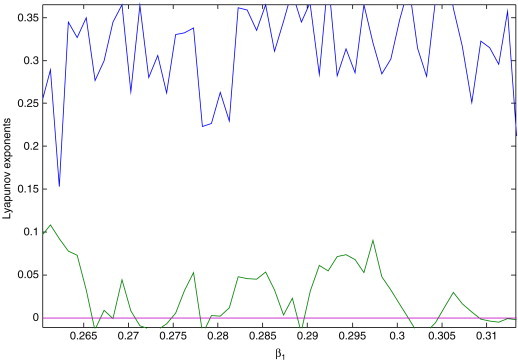
Local amplification of Fig. 3b for neighborhood ${\beta }_1=0.28$.

Assume that ${\lambda }_j(j=1,2,3,4,5)$ are Lyapunov exponents of system (2.3), satisfying the condition ${\lambda }_1\ge {\lambda }_2\ge {\lambda }_3\ge {\lambda }_4\ge {\lambda }_5$. The dynamical behaviors of system (2.3) based on the Lyapunov exponents are given in Table 1 .

Table 1.

Attractor type of system (2.3) based on the Lyapunov exponents.

Lyapunov exponents	Attractor type
${\lambda }_1>0,{\lambda }_2>0,{\lambda }_3=0,{\lambda }_4<0,{\lambda }_5<0$	Hyperchaotic attractor
${\lambda }_1>0,{\lambda }_2=0,{\lambda }_3<0,{\lambda }_4<0,{\lambda }_5<0$	Chaotic attractor
${\lambda }_1=0,{\lambda }_2<0,{\lambda }_3<0,{\lambda }_4<0,{\lambda }_5<0$	Period attractor

Hyperchaotic dynamical behavior is analyzed via phase plots as follows. The projection of a hyperchaotic attractor on phase plan of system (2.3) with ${\beta }_1=0.28$ is given in Fig. 4 .

Fig. 4.

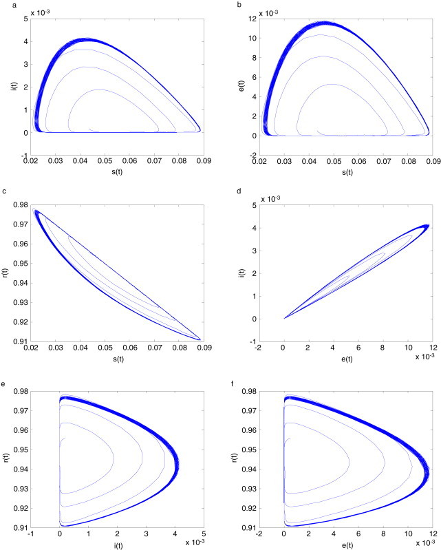
The projection of a hyperchaotic attractor of system (2.3) with systemic parameter ${\beta }_1=0.28$ on plane (a) $s\text{–}i$; (b) $s\text{–}e$; (c) $s\text{–}r$; (d) $e\text{–}i$; (e) $i\text{–}r$; (f) $e\text{–}r$.

The hyperchaotic attractor of system (2.3) with ${\beta }_1=0.28$ is shown in Fig. 5 .(a), (b), (c) and (d). The Poincare section of system (2.3) with ${\beta }_1=0.28$ is given in Fig. 6 .

Fig. 5.

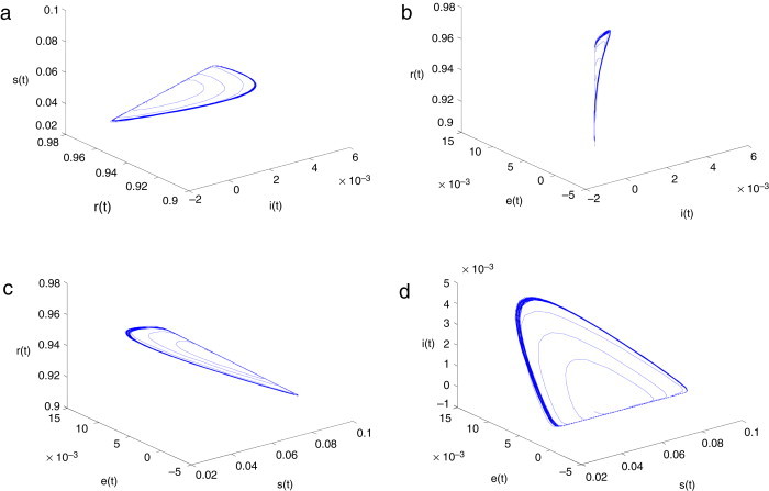
Hyperchaotic attractor of system (2.3) with parameter ${\beta }_1=0.28$.(a) $i\text{–}r\text{–}s$; (b) $i\text{–}e\text{–}r$; (c) $s\text{–}e\text{–}r$; (d) $s\text{–}e\text{–}i$.

Fig. 6.

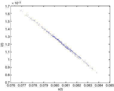
Poincare section of system (2.3) with ${\beta }_1=0.28$.

3.1.2. Two and three varying parameter

It is well known that systemic parameters vary in many practical problems. In this subsection, we consider the cases of two and three varying parameters. Broer et al. [37], [38] introduce an algorithm on Lyapunov diagram and the diagram is used to scan the parameter plan. To observe clearly the dynamical behaviors, Lyapunov diagrams Fig. 7, Fig. 8 . are applied in our paper. A Lyapunov diagram is a plot of a two-parameter plane, where each color corresponds to one type of attractor, classified on the basis of Lyapunov exponents ${\lambda }_1\ge {\lambda }_2\ge {\lambda }_3\ge {\lambda }_4\ge {\lambda }_5$, according to the color code in Table 2.

Fig. 7.

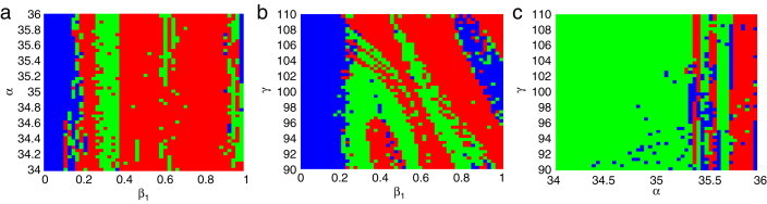
Lyapunov diagram of system (2.3) (a) in the ${\beta }_1\text{–}\alpha$ parameter plane; (b) in the ${\beta }_1\text{–}\gamma$ parameter plane; (c) in $\alpha \text{–}\gamma$ parameter plane. For the color code see Table 2. (For interpretation of the references to colour in this figure legend, the reader is referred to the web version of this article.)

Fig. 8.

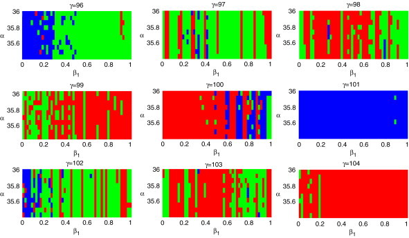
Lyapunov diagram of system (2.3) with the parameter $\gamma =96:1:104$ in the ${\beta }_1\text{–}\alpha$ parameter plane. For the color code see Table 2. (For interpretation of the references to colour in this figure legend, the reader is referred to the web version of this article.)

Table 2.

Legend of the color coding for Fig. 7, Fig. 8: the attractors are classified by means of Lyapunov exponents (${\lambda }_1,{\lambda }_2,{\lambda }_3,{\lambda }_4,{\lambda }_5$).

Colour	Lyapunov exponents	Attractor type
Red	${\lambda }_1\ge {\lambda }_2>{\lambda }_3=0>{\lambda }_4\ge {\lambda }_5$	Hyperchaotic attractor
Green	${\lambda }_1>{\lambda }_2=0>{\lambda }_3\ge {\lambda }_4\ge {\lambda }_5$	Chaotic attractor
Blue	${\lambda }_1=0>{\lambda }_2\ge {\lambda }_3\ge {\lambda }_4\ge {\lambda }_5$	Period attractor

For the case of two varying parameters, we discuss three sub-cases as follows.

• (1)Fixing $b=0.02$, ${\beta }_0=1800$ and $\gamma =100$, let the parameter ${\beta }_1$ and $\alpha$ be varying parameters. Taking ${\beta }_1\in [0,1]$ and $\alpha \in [34,36]$, the Lyapunov diagram is given in Fig. 7(a).
• (2)Fixing $b=0.02$, ${\beta }_0=1800$ and $\alpha =35.84$, let the parameter ${\beta }_1$ and $\gamma$ be varying parameters. Taking ${\beta }_1\in [0,1]$ and $\gamma \in [90,110]$, the Lyapunov diagram is shown in Fig. 7(b).
• (3)Fixing $b=0.02$, ${\beta }_0=1800$ and ${\beta }_1=0.28$, let the parameter $\alpha$ and $\gamma$ be varying parameters. Taking $\alpha \in [34,36]$ and $\gamma \in [90,110]$, the Lyapunov diagram is given in Fig. 7(c).

For the case of three varying parameters, fixing the parameter $b=0.02$, ${\beta }_0=1800$ and taking ${\beta }_1\in [0,1]$, $\alpha \in [35.5,36]$ and $\gamma \in [96,104]$, the Lyapunov diagram is shown in Fig. 8.

According to the above-mentioned analysis, we know that system (2.3) has very complicated dynamical behaviors, such as period, chaos and hyperchaos phenomena with some parameter values, respectively.

Hyperchaotic dynamical behavior is similar to chaotic dynamical behavior, and multi-stability coexists in a system. A hyperchaotic attractor has a multi-direction adjacent orbit exponent divergent characteristic, as well as the complex characteristic of a high tangle orbit. From Fig. 4, Fig. 5, Fig. 6, the hyperchaotic attractor has not only the general characteristic of a low dimension chaotic attractor, but also has the following speciality: hyperchaotic systems have shrinkable or radiation behavior at least on a plane or loop plane. Hereby, the projections of hyperchaotic attractor on a phase plane are of more complicated fold and tensible trajectories. It is shown that the instability in local region of hyperchaotic systems is stronger than in low dimension chaotic systems. Hence, the control difficulty of hyperchaotic systems is increased.

The biologic signification of hyperchaos in epidemic models is that, the epidemic disease will break out suddenly and spread gradually in a region at the period of the high incidence of the epidemic disease. This means that many people in the region will be infected by disease, and some of them could even lose their lives. Nevertheless, there exists an uncertain prediction for the low period of the incidence of the epidemic disease. Therefore, it is important to control the hyperchaos of the epidemic model.

3.2. Hyperchaos control

In this subsection, we will control the hyperchaos for system (2.3) and design a tracking controller $u\left(t\right)$ so that $i\left(t\right)\to 0$ when $t\to \infty$. That is, the disease gradually disappears and our aim is reached.

It is well known that there are three conditions for epidemic transmission, i.e., sources of infection, route of transmission and a susceptible population. If we understand rightly the rule of the epidemic process of epidemic disease, take timely valid measures and prevent any one of the three conditions from being produced, the transmission of epidemic disease can be prevented. Therefore, we can reach the aim of controlling and eliminating epidemic disease. The susceptible, the body for certain diseases that is lower or has a lack of immunity, cannot resist the invasion of certain pathogens. The higher the percentage of the susceptible is, the larger is the possibility of disease outbreaks. Therefore, it is important to control the susceptible and it is easy to implement this measure.

The new controlled system has the form of

$$s^{\prime }\left(t\right)=b(1-s\left(t\right))-{\beta }_0(1+{\beta }_{1}cos2\pi t)s\left(t\right)i\left(t\right)+u\left(t\right)$$$$e^{\prime }\left(t\right)={\beta }_0(1+{\beta }_{1}cos2\pi t)s\left(t\right)i\left(t\right)-(\alpha +b)e\left(t\right)$$$$i^{\prime }\left(t\right)=\alpha e\left(t\right)-(\gamma +b)i\left(t\right)$$$$0=s\left(t\right)+e\left(t\right)+i\left(t\right)+r\left(t\right)-1\text{.}$$ (3.1)

To simplify, we take the transformation $x\left(t\right)=2\pi t$, the nonautonomy system (3.1) is equivalent to the following autonomy system:

$$s^{\prime }\left(t\right)=b(1-s\left(t\right))-{\beta }_0(1+{\beta }_{1}cosx\left(t\right))s\left(t\right)i\left(t\right)+u\left(t\right)$$$$e^{\prime }\left(t\right)={\beta }_0(1+{\beta }_{1}cosx\left(t\right))s\left(t\right)i\left(t\right)-(\alpha +b)e\left(t\right)$$$$i^{\prime }\left(t\right)=\alpha e\left(t\right)-(\gamma +b)i\left(t\right)$$$$x^{\prime }\left(t\right)=2\pi$$$$0=s\left(t\right)+e\left(t\right)+i\left(t\right)+r\left(t\right)-1\text{.}$$ (3.2)

System (3.2) can be written as the standard form of system (2.4). So let $X\left(t\right)={(s\left(t\right),e\left(t\right),i\left(t\right),x\left(t\right))}^T$, $Y\left(t\right)=r\left(t\right)$,

$$f(X\left(t\right),Y\left(t\right))=\left[\begin{array}{c}\hfill b(1-s\left(t\right))-{\beta }_0(1+{\beta }_{1}cosx\left(t\right))s\left(t\right)i\left(t\right)\hfill \\ \hfill {\beta }_0(1+{\beta }_{1}cosx\left(t\right))s\left(t\right)i\left(t\right)-(\alpha +b)e\left(t\right)\hfill \\ \hfill \alpha e\left(t\right)-(\gamma +b)i\left(t\right)\hfill \\ \hfill 2\pi \hfill \end{array}\right]\text{,}g(X\left(t\right),Y\left(t\right))=\left[\begin{array}{c}\hfill 1\hfill \\ \hfill 0\hfill \\ \hfill 0\hfill \\ \hfill 0\hfill \end{array}\right]\text{,}$$

$$p(X\left(t\right),Y\left(t\right))=s\left(t\right)+e\left(t\right)+i\left(t\right)+r\left(t\right)-1\text{.}$$

According to the definition of $M$ derivative, take the output $h(X\left(t\right),Y\left(t\right))=i\left(t\right)$ of system (3.2), and we obtain

$$M_g{M}_f^{0}h(X\left(t\right),Y\left(t\right))=M_g{M}_f^{0}i\left(t\right)=0\text{,}$$

$$M_g{M}_{f}h(X\left(t\right),Y\left(t\right))=0\text{,}$$

$$M_g{M}_f^{2}h(X\left(t\right),Y\left(t\right))=\alpha {\beta }_0(1+{\beta }_{1}cosx\left(t\right))i\left(t\right)\ne 0\text{.}$$

It shows that the relative degree is 3.

Take the following coordinate transformation,

$${\xi }_1\left(t\right)=i\left(t\right)\text{,}$$$${\xi }_2\left(t\right)=\alpha e\left(t\right)-(\gamma +b)i\left(t\right)\text{,}$$$${\xi }_3\left(t\right)=\alpha {\beta }_0(1+{\beta }_{1}cosx\left(t\right))s\left(t\right)i\left(t\right)-\alpha (\alpha +2b+\gamma )e\left(t\right)+{(\gamma +b)}^{2}i\left(t\right)\text{,}$$$$x\left(t\right)=2\pi t\text{.}$$ (3.3)

We can get the following standard form:

$${\dot{\xi }}_1\left(t\right)={\xi }_2\left(t\right)$$$${\dot{\xi }}_2\left(t\right)={\xi }_3\left(t\right)$$$${\dot{\xi }}_3\left(t\right)=\overline{\upsilon }\left(t\right)$$$$\dot{x}\left(t\right)=2\pi$$$$0=\frac{\alpha +\gamma +b}{\alpha }{\xi }_1\left(t\right)+\frac{1}{\alpha }{\xi }_2\left(t\right)+\sigma \left(t\right)+r\left(t\right)-1$$ (3.4)

where

$$\sigma \left(t\right)=\frac{1}{\alpha {\beta }_0(1+{\beta }_{1}cosx\left(t\right)){\xi }_1\left(t\right)}[(\alpha +b)(\gamma +b){\xi }_1\left(t\right)+(\alpha +2b+\gamma ){\xi }_2\left(t\right)+{\xi }_3\left(t\right)]\text{,}$$

$$\overline{\upsilon }\left(t\right)=[\frac{{\xi }_2\left(t\right)}{{\xi }_1\left(t\right)}+\frac{2\pi {\beta }_{1}sinx\left(t\right)}{1+{\beta }_{1}cosx\left(t\right)}-{\beta }_0(1+{\beta }_{1}cosx\left(t\right)){\xi }_1\left(t\right)][(\alpha +b)(\gamma +b){\xi }_1\left(t\right)+(\alpha +2b+\gamma ){\xi }_2\left(t\right)+{\xi }_3\left(t\right)]+b[\alpha {\beta }_0(1+{\beta }_{1}cosx\left(t\right))-2(\alpha +b)(\gamma +b)]{\xi }_1\left(t\right)+[\gamma +b-(\gamma +2b)(\alpha +2b+\gamma )]{\xi }_2\left(t\right)-(\alpha +3b+\gamma ){\xi }_3\left(t\right)+\alpha {\beta }_0(1+{\beta }_{1}cosx\left(t\right)){\xi }_1\left(t\right)u\left(t\right)\text{.}$$

Obviously, it shows that the differential equations of system (3.2) are divided into a linear subsystem of input–output behavior (that is from the first to third differential equations of system (3.4)), where the dimension is 3 and the other subsystem with dimension 1 (that is the fourth differential equation of system (3.4)), but this subsystem does not affect the output of system (3.2). In order to research the output tracking of system (3.2), we only consider from the first to third differential equations of system (3.4) and the algebraic restrict equation. Our aim is that the output trajectory of system (3.2) tracks an ideal state $i_d\left(t\right)=0$, this means the disease gradually disappears.

Theorem 3.1

The controller of controlled system (3.2) is

$$u\left(t\right)=\frac{1}{\alpha {\beta }_0(1+{\beta }_{1}cos2\pi t)i\left(t\right)}[-Z(s\left(t\right),e\left(t\right),i\left(t\right))+\upsilon \left(t\right)]$$ (3.5)

where

$$Z(s\left(t\right),e\left(t\right),i\left(t\right))=\alpha {\beta }_0(1+{\beta }_{1}cos2\pi t)i\left(t\right)[b-(\alpha +4b+2\gamma )s\left(t\right)-{\beta }_0(1+{\beta }_{1}cos2\pi t)s\left(t\right)i\left(t\right)]+\alpha e\left(t\right)[\alpha {\beta }_0(1+{\beta }_{1}cos2\pi t)s\left(t\right)+(\alpha +b)(\alpha +2b+\gamma )+{(\gamma +b)}^2]-{(\gamma +b)}^{3}i\left(t\right)-2\pi \alpha {\beta }_0{\beta }_{1}s\left(t\right)i\left(t\right)sin2\pi t\text{,}$$

$$\upsilon \left(t\right)=-c_{0}i\left(t\right)-c_1[\alpha e\left(t\right)-(\gamma +b)i\left(t\right)]-c_2[\alpha {\beta }_0(1+{\beta }_{1}cos2\pi t)s\left(t\right)i\left(t\right)-\alpha (\alpha +2b+\gamma )e\left(t\right)+{(\gamma +b)}^{2}i\left(t\right)]\text{,}$$

where the constants $c_0,c_1,c_2$ satisfy that all roots of equation $p^3+c_2{p}^2+c_{1}p+c_0=0$ lie the left half plane of $p$ , the output of system (3.2) $h(X\left(t\right),Y\left(t\right))=i\left(t\right)\to 0$ when $t\to \infty$.

Proof

Let the error variable $\omega \left(t\right)={({\omega }_1\left(t\right),{\omega }_2\left(t\right),{\omega }_3\left(t\right))}^T\in {\mathbb{R}}^3$,

$$\omega \left(t\right)=\xi \left(t\right)-{\xi }_d\left(t\right)\text{,}$$

where $\xi \left(t\right)={({\xi }_1\left(t\right),{\xi }_2\left(t\right),{\xi }_3\left(t\right))}^T,{\xi }_d\left(t\right)={({\xi }_{1d}\left(t\right),{\xi }_{2d}\left(t\right),{\xi }_{3d}\left(t\right))}^T={(i_d\left(t\right),i_d^{\prime }\left(t\right),i_d^{″}\left(t\right))}^T$.

We can get the following error system:

$${\dot{\omega }}_1\left(t\right)={\omega }_2\left(t\right)$$$${\dot{\omega }}_2\left(t\right)={\omega }_3\left(t\right)$$$${\dot{\omega }}_3\left(t\right)=\overline{\upsilon }\left(t\right)$$$$\dot{x}\left(t\right)=2\pi$$$$0=\frac{\alpha +\gamma +b}{\alpha }{\omega }_1\left(t\right)+\frac{1}{\alpha }{\omega }_2\left(t\right)+\theta \left(t\right)+r\left(t\right)-1$$ (3.6)

where $\theta \left(t\right)=\frac{1}{\alpha {\beta }_0(1+{\beta }_{1}cosx\left(t\right)){\omega }_1\left(t\right)}[(\alpha +b)(\gamma +b){\omega }_1\left(t\right)+(\alpha +2b+\gamma ){\omega }_2\left(t\right)+{\omega }_3\left(t\right)]$,

Substituting (3.3), (3.5) into (3.6), we can obtain the following subsystem:

$${\dot{\omega }}_1\left(t\right)={\omega }_2\left(t\right)$$$${\dot{\omega }}_2\left(t\right)={\omega }_3\left(t\right)$$$${\dot{\omega }}_3\left(t\right)=\upsilon \left(t\right)$$ (3.7)

where $\upsilon =-c_0{\omega }_1\left(t\right)-c_1{\omega }_2\left(t\right)-c_2{\omega }_3\left(t\right)$, according to the theory of [39], choose appropriate constants $c_0,c_1,c_2$ satisfying all roots of equation $p^3+c_2{p}^2+c_{1}p+c_0=0$ that lie in the left half plane of $p$, thus subsystem (3.7) after feedback is an asymptotically stable system. That is $\omega \left(t\right)\to 0$ when $t\to \infty$, thus $i\left(t\right)\to 0$ when $t\to \infty$, that means the output of system tracking ideal trajectory is $i_d\left(t\right)=0$. This completes the proof. □

Remark 3

There is important practical significance of the control for the susceptible in Theorem 3.1. First, we can be vaccinated for the susceptible and enhance immunity by taking exercise. Second, it is necessary to decrease contact with the infectious.

3.3. Case ${\beta }_1=0$

In this subsection, we discuss the stabilities of trivial equilibria and nontrivial equilibria for system (2.3) with ${\beta }_1=0$, respectively. We further study the bifurcation of the system and design a isolation control such that the disease is eliminated gradually.

The system (2.3) with ${\beta }_1=0$ can be written

$$s^{\prime }=b-bs-{\beta }_{0}si$$$$e^{\prime }={\beta }_{0}si-(\alpha +b)e$$$$i^{\prime }=\alpha e-(\gamma +b)i$$$$0=s+e+i+r-1\text{.}$$ (3.8)

To obtain the equilibria of system (3.8), let

$$b-bs-{\beta }_{0}si=0,{\beta }_{0}si-(\alpha +b)e=0,\alpha e-(\gamma +b)i=0,s+e+i+r-1=0\text{.}$$

We get the disease-free equilibrium $P_0(1,0,0,0)$ and the endemic equilibrium $P_1(s^{\ast },e^{\ast },i^{\ast },r^{\ast })$, where $s^{\ast }=\frac{b}{b+{\beta }_0{i}^{\ast }}$, $e^{\ast }=\frac{\gamma +b}{\alpha }{i}^{\ast }$, $i^{\ast }=\frac{\alpha b}{(\alpha +b)(\gamma +b)}-\frac{b}{{\beta }_0}$, $r^{\ast }=\frac{b}{\gamma }{i}^{\ast }$.

For simplicity, let $f(X_1,Y_1,{\beta }_0)=\left[\begin{array}{c}\hfill b-bs-{\beta }_{0}si\hfill \\ \hfill {\beta }_{0}si-(\alpha +b)e\hfill \\ \hfill \alpha e-(\gamma +b)i\hfill \end{array}\right]$, $g(X_1,Y_1,{\beta }_0)=s+e+i+r-1$,

where $X_1={[s,e,i]}^T$, $Y_1=r$ and ${\beta }_0$ is a bifurcation parameter of system (3.8). Since $D_{Y_1}g=1\ne 0$, we can get

$$\Sigma =D_{X_1}f-D_{Y_1}f{\left(D_{Y_1}g\right)}^{-1}{D}_{X_1}g=\left[\begin{array}{ccc}\hfill -b-{\beta }_{0}i\hfill & \hfill 0\hfill & \hfill -{\beta }_{0}s\hfill \\ \hfill {\beta }_{0}i\hfill & \hfill -(\alpha +b)\hfill & \hfill {\beta }_{0}s\hfill \\ \hfill 0\hfill & \hfill \alpha \hfill & \hfill -(\gamma +b)\hfill \end{array}\right]\text{.}$$

The following theorem shows the stability of disease-free equilibrium $P_0(1,0,0,0)$.

Theorem 3.2

The disease-free equilibrium $P_0(1,0,0,0)$ of system (3.8) is globally asymptotically stable in $\Gamma$ if ${\beta }_0<{\beta }_0^{\ast }$ ; it is unstable if ${\beta }_0>{\beta }_0^{\ast }$ , where ${\beta }_0^{\ast }=\frac{(\alpha +b)(\gamma +b)}{\alpha }$.

Proof

The Jacobian matrix of system (3.8) at the equilibrium $P_0$ is

$${\Sigma }_{P_0}=\left[\begin{array}{ccc}\hfill -b\hfill & \hfill 0\hfill & \hfill -{\beta }_0\hfill \\ \hfill 0\hfill & \hfill -(\alpha +b)\hfill & \hfill {\beta }_0\hfill \\ \hfill 0\hfill & \hfill \alpha \hfill & \hfill -(\gamma +b)\hfill \end{array}\right]$$

and we can get the characteristic equation of ${\Sigma }_{P_0}$,

$$|\lambda {\rm Y}-{\Sigma }_{P_0}|=(\lambda +b)[{\lambda }^2+(\alpha +\gamma +2b)\lambda +(\alpha +b)(\gamma +b)-\alpha {\beta }_0]=0$$

where ${\rm Y}$ is a unit matrix.

We can see that one of the eigenvalues is $-b$ and the other two are the roots of

$${\lambda }^2+(\alpha +\gamma +2b)\lambda +(\alpha +b)(\gamma +b)-\alpha {\beta }_0=0\text{.}$$

If ${\beta }_0<{\beta }_0^{\ast }$, all three eigenvalues have negative real parts and the equilibrium $P_0$ is locally asymptotically stable. If ${\beta }_0>{\beta }_0^{\ast }$, the nontrivial equilibrium emerges and the trivial equilibrium $P_0$ becomes unstable. There are positive real parts of two eigenvalues. The equilibrium $P_0$ is unstable. This completes the proof.  □

Theorem 3.3

If ${\beta }_0>{\beta }_0^{\ast }$ , the equilibrium $P_1$ of system (3.8) is locally asymptotically stable; if ${\beta }_0<{\beta }_0^{\ast },P_1$ is unstable.

Proof

The Jacobian matrix of system (3.8) at $P_1$

$${\Sigma }_{P_1}=\left[\begin{array}{ccc}\hfill -b-{\beta }_0{i}^{\ast }\hfill & \hfill 0\hfill & \hfill -{\beta }_0{s}^{\ast }\hfill \\ \hfill {\beta }_0{i}^{\ast }\hfill & \hfill -(\alpha +b)\hfill & \hfill {\beta }_0{s}^{\ast }\hfill \\ \hfill 0\hfill & \hfill \alpha \hfill & \hfill -(\gamma +b)\hfill \end{array}\right]\text{.}$$

The characteristic equation of ${\Sigma }_{P_1}$ is

$$|\lambda {\rm Y}-{\Sigma }_{P_1}|={\lambda }^3+C_1{\lambda }^2+C_2\lambda +C_3=0$$

where

$$C_1=\alpha +\gamma +2b+\frac{\alpha b{\beta }_0}{(\alpha +b)(\gamma +b)}\text{,}$$

$$C_2=\frac{\alpha b{\beta }_0}{(\alpha +b)(\gamma +b)}(\alpha +\gamma +2b)\text{,}$$

$$C_3=b[\alpha {\beta }_0-(\alpha +b)(\gamma +b)]\text{,}$$

when ${\beta }_0>{\beta }_0^{\ast }$, the conditions of the Routh–Hurwitz criterion are satisfied. Then, the equilibrium $P_1$ is locally asymptotically stable. When ${\beta }_0<{\beta }_0^{\ast }$, there exists one or three positive eigenvalues. The equilibrium $P_1$ is unstable. This completes the proof.  □

Remark 4

According to Theorem 3.2, Theorem 3.3, we note that if ${\beta }_0<{\beta }_0^{\ast }$, the system (3.8) is stable at the equilibrium $P_0$, which corresponds to the disappearance of the disease. If ${\beta }_0>{\beta }_0^{\ast }$, the system (3.8) is stable at the equilibrium $P_1$ which the endemic disease is formed. The stability of the equilibrium $P_0$ produces the transformation at ${\beta }_0={\beta }_0^{\ast }$. It shows that a bifurcation may happen at ${\beta }_0={\beta }_0^{\ast }$.

Theorem 3.4

The system (3.8) undergoes transcritical bifurcation at the disease-free equilibrium $P_0$ , when the bifurcation parameter ${\beta }_0$ is ${\beta }_0^{\ast }$.

Proof

When the bifurcation parameter ${\beta }_0={\beta }_0^{\ast }$, the matrix

$${\Sigma }_{P_0}=\left[\begin{array}{ccc}\hfill -b\hfill & \hfill 0\hfill & \hfill -\frac{(\alpha +b)(\gamma +b)}{\alpha }\hfill \\ \hfill 0\hfill & \hfill -(\alpha +b)\hfill & \hfill \frac{(\alpha +b)(\gamma +b)}{\alpha }\hfill \\ \hfill 0\hfill & \hfill \alpha \hfill & \hfill -(\gamma +b)\hfill \end{array}\right]$$

has a geometrically simple zero eigenvalue with right eigenvector $\Phi ={\left[\begin{array}{ccc}\hfill -\frac{(\alpha +b)(\gamma +b)}{\alpha b}\hfill & \hfill \frac{\gamma +b}{\alpha }\hfill & \hfill 1\hfill \end{array}\right]}^T$ and left eigenvector $\Psi =\left[\begin{array}{ccc}\hfill 0\hfill & \hfill \frac{\alpha }{\alpha +b}\hfill & \hfill 1\hfill \end{array}\right]$. There is no other eigenvalue on the imaginary axis and

$$\Psi \left(D_{{\beta }_0{X}_1}f\right)\Phi =\frac{\alpha }{\alpha +b}\ne 0\text{,}$$

$$\Psi \left(\left(D_{X_1{X}_1}f\right)(\Phi ,\Phi )\right)=-\frac{2(\alpha +b){(\gamma +b)}^2}{\alpha b}\ne 0\text{.}$$

According to the literature [40], system (3.8) undergoes transcritical bifurcation at the disease-free equilibrium $P_0$. This completes the proof. □

Remark 5

Note that when ${\beta }_0={\beta }_0^{\ast }$, the endemic equilibrium $P_1$ translates the disease-free equilibrium $P_0$. We must effectively control the transmission rate ${\beta }_0$, such that the value ${\beta }_0$ is less than ${\beta }_0^{\ast }$. It is important to effectively control the value ${\beta }_0$.

We take the isolation control method to reach our aim. Taking isolation control, then the system (3.8) can be written

$$s^{\prime }=b-bs-({\beta }_0-\eta )si$$$$e^{\prime }=({\beta }_0-\eta )si-(\alpha +b)e$$$$i^{\prime }=\alpha e-(\gamma +b)i$$$$0=s+e+i+r-1$$ (3.9)

where the isolation rate $0<\eta <{\beta }_0$.

According to Theorem 3.2, Theorem 3.3, Theorem 3.4, we know that if ${\beta }_0-\eta <{\beta }_0^{\ast }$, the system (3.9) is stable at $P_0$; if ${\beta }_0-\eta >{\beta }_0^{\ast }$, the system (3.9) is stable at $P_1$. Obviously, when ${\beta }_0-{\beta }_0^{\ast }<\eta <{\beta }_0$, the aim of elimination of the disease can be reached, and it is easy to implement in real life. Nevertheless, the investments in human, material and financial resources are larger as the isolation rate increases, and it is hard to realize. Therefore, we take the isolation rate $\eta \to {\beta }_0-{\beta }_0^{\ast }$ to achieve our aim.

Remark 6

By enhancing the immunity of the susceptible, quarantining the infectious and decreasing contact between the infectious and the susceptible, we can obtain the isolation rate $\eta$.

3.4. Numerical simulation

In this subsection, numerical examples are used to demonstrate the validity of the controller.

Case I. The parameters of system (2.3) are supposed as follows:

$$b=0.02\text{,}\alpha =35.84\text{,}\gamma =100\text{,}{\beta }_0=1800\text{,}{\beta }_1=0.28\text{.}$$

In this case, the system (2.3) is hyperchaotic. According to Theorem 3.1, we design the controller of controlled system (3.1)

$$u\left(t\right)=\frac{1}{35.84\times 1800(1+0.28cos2\pi t)i\left(t\right)}[-Z(s\left(t\right),e\left(t\right),i\left(t\right))+\upsilon \left(t\right)]$$

where

$$Z(s\left(t\right),e\left(t\right),i\left(t\right))=64512(1+0.28cos2\pi t)i\left(t\right)[0.02-235.92s\left(t\right)-1800(1+0.28cos2\pi t)s\left(t\right)i\left(t\right)]+35.84e\left(t\right)[64512(1+0.28cos2\pi t)s\left(t\right)+14873.9396]-100.{02}^{3}i\left(t\right)-36126.72\pi s\left(t\right)i\left(t\right)sin2\pi t\text{,}$$

$$\upsilon \left(t\right)=-c_{0}i\left(t\right)-c_1[35.84e\left(t\right)-100.02i\left(t\right)]-c_2[64512(1+0.28cos2\pi t)s\left(t\right)i\left(t\right)-4869.9392e\left(t\right)+100.{02}^{2}i\left(t\right)]\text{,}$$

choose $c_0=6,c_1=11,c_2=6$ satisfying all roots of equation $p^3+c_2{p}^2+c_{1}p+c_0=0$ lie in the left half plane of $p$, the figures of $i\left(t\right)$ trajectory with an uncontrolled system and a controlled system are shown in Fig. 9a, Fig. 9b .

Fig. 9a.

The dynamic response of $i\left(t\right)$ trajectory under an uncontrolled system.

Fig. 9b.

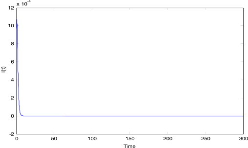
The dynamic response of $i\left(t\right)$ trajectory under a controlled system.

From Fig. 9b, we can see easily that the infectious trajectory of system (3.1) tracks an ideal state $i_d\left(t\right)=0$ via designing a tracking controller and it is shown that the disease will gradually disappear.

Case II. The parameters of system (3.8) are supposed as follows:

$$b=0.02\text{,}\alpha =35.84\text{,}\gamma =100\text{,}{\beta }_0=180\text{.}$$

By calculating, we get ${\beta }_0^{\ast }=100.0758$. Making a different isolation rate $\eta$, the response of $i\left(t\right)$ is shown in Fig. 10 .

Fig. 10.

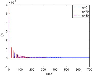
The response of $i\left(t\right)$ of system (3.9) for a different isolation rate $\eta$ at initial value (0.579, 0.02, 0.001, 0.4).

From Fig. 10, we can see that the larger the isolation rate $\eta$ is, the better the effect of control is, and the smaller the infection is. When $\eta =70<{\beta }_0-{\beta }_0^{\ast }$, the controlled system is stable at the endemic equilibrium. It shows that the endemic disease forms. When $\eta =80>{\beta }_0-{\beta }_0^{\ast }$, number of the infectives gradually becomes zero with time, i.e. , when ${\beta }_0-\eta \to {\beta }_0^{\ast }$, the disease is eliminated ultimately. To avoid forming an endemic disease at certain region, isolation control is an effective measure. This is also a common method.

4. Conclusions

Bifurcation or chaos dynamical behavior exists in many epidemic models. These dynamical behaviors are generally deleterious for biologic systems, and often lead to a disease spreading gradually or breaking out suddenly in certain regions. In other words, many people in the region would be infected by disease and some of them could even lose their lives. Therefore, it is important to effectively control bifurcation or chaotic dynamical behavior of epidemic models.

In this paper, we study an SEIR epidemic model which is a differential and algebraic system with seasonal forcing in transmission rate. We consider three cases: only one varying parameter, two varying parameters and three varying parameters. For the case of only one varying parameter, we analyze the dynamics of the system by using the bifurcation diagrams, Lyapunov exponent spectrum diagram and Poincare section. For the cases of two and three varying parameters, a Lapunov diagram is applied in the analysis of dynamical behaviors. Furthermore, for the hyperchaotic dynamical behavior of the system, we design a tracking controller such that the disease gradually disappears. In particular, we discuss the stability and the transcritical bifurcation for the degree of seasonality ${\beta }_1=0$. The disease is eliminated by taking isolation control which is an effective measure. Finally, numerical simulations are given to illuminate the proposed control methods.

References

- 1.Fan M., Michael Y.L., Wang K. Global stability of an SEIS epidemic model with recruitment and a varying total population size. Mathematical Biosciences. 2001;170:199–208. doi: 10.1016/s0025-5564(00)00067-5. [DOI] [PubMed] [Google Scholar]
- 2.Chen L.S., Chen J. Science Press; Beijing: 1993. Nonlinear Biologic Dynamic Systems. [Google Scholar]
- 3.Li X.Z., Gupur G., Zhu G.T. Threshold and stability results for an age-structured SEIR epidemic model. Computers & Mathematics with Applications. 2001;42:883–907. [Google Scholar]
- 4.May R.M., Oster G.F. Bifurcation and dynamic complexity in simple ecological models. American Naturalist. 1976;110:573–599. [Google Scholar]
- 5.Zeng G.Z., Chen L.S., Sun L.H. Complexity of an SIRS epidemic dynamics model with impulsive vaccination control. Chaos Solitons & Fractals. 2005;26:495–505. [Google Scholar]
- 6.Lu Z.H., Liu X.N., Chen L.S. Hopf bifurcation of nonlinear incidence rates SIR epidemiological models with stage structure. Communications in Nonlinear Science & Numerical Simulation. 2001;6:205–209. [Google Scholar]
- 7.Ghoshal G., Sander L.M., Sokolov I.M. SIS epidemics with household structure: the self-consistent field method. Mathematical Biosciences. 2004;190:71–85. doi: 10.1016/j.mbs.2004.02.006. [DOI] [PubMed] [Google Scholar]
- 8.Hilker F.M., Michel L., Petrovskii S.V., Malchow H. A diffusive SI model with Allee effect and application to FIV. Mathematical Biosciences. 2007;206:61–80. doi: 10.1016/j.mbs.2005.10.003. [DOI] [PubMed] [Google Scholar]
- 9.Greenhalgh D., Khan Q.J.A., Lewis F.I. Hopf bifurcation in two SIRS density dependent epidemic models. Mathematical and Computer Modelling. 2004;39:1261–1283. [Google Scholar]
- 10.Glendinning P., Perry L.P. Melnikov analysis of chaos in a simple epidemiological model. Journal of Mathematical Biology. 1997;35:359–373. doi: 10.1007/s002850050056. [DOI] [PubMed] [Google Scholar]
- 11.Michael Y.L., Graef J.R., Wang L.C., Karsai J. Global dynamics of an SEIR model with varying total population size. Mathematical Biosciences. 1999;160:191–213. doi: 10.1016/s0025-5564(99)00030-9. [DOI] [PubMed] [Google Scholar]
- 12.Kuznetsov Y.A., Piccardi C. Bifurcation analysis of periodic SEIR and SIR epidemic models. Mathematical Biosciences. 1994;32:109–121. doi: 10.1007/BF00163027. [DOI] [PubMed] [Google Scholar]
- 13.Olsen L.F., Schaffer W.M. Chaos versus periodicity: alternative hypotheses for childhood epidemics. Science. 1990;249:499–504. doi: 10.1126/science.2382131. [DOI] [PubMed] [Google Scholar]
- 14.Sun C.J., Lin Y.P., Tang S.P. Global stability for an special SEIR epidemic model with nonlinear incidence rates. Chaos Solitons & Fractals. 2007;33:290–297. [Google Scholar]
- 15.Xu W.B., Liu H.L., Yu J.Y., Zhu G.T. Stability results for an age-structured Seir Epidemic model. Journal of Systems Science and Information. 2005;3:635–642. [Google Scholar]
- 16.Liu W.M., Hethcote H.W., Levin S.A. Dynamical behavior of epidemiological models with nonlinear incidence rates. Journal of Mathematical Biology. 1987;25:359–380. doi: 10.1007/BF00277162. [DOI] [PubMed] [Google Scholar]
- 17.Greenhalgh D. Hopf bifurcation in epidemic models with a latent period and non-permanent immunity. Mathematical and Computer Modelling. 1997;25:85–107. [Google Scholar]
- 18.Cooke K.L., Driessche P.V. Analysis of an SEIRS epidemic model with two delays. Journal of Mathematical Biology. 1996;35:240–260. doi: 10.1007/s002850050051. [DOI] [PubMed] [Google Scholar]
- 19.Venkatasubramanian V., Schattler H., Zaborszky J. Analysis of local bifurcation mechanisms in large differential-algebraic systems such as the power system. Proceedings of the 32nd Conference on Decision and Control. 1993;4:3727–3733. [Google Scholar]
- 20.Rosehart W.D., Canizares C.A. Bifurcation analysis of various power system models. Electrical Power and Energy Systems. 1999;21:171–182. [Google Scholar]
- 21.Zhang J.S. Qing Hua University press; Beijing: 1990. Economy Cybernetics of Singular Systems. [Google Scholar]
- 22.Dai L. Springer-Verlag; Heidelberg: 1998. Singular Control Systems. New York. [Google Scholar]
- 23.Kermack W.O., McKendrick A.G. A contribution to the mathematical theory of epidemics. Proceedings of the Royal Society of London A. 1927;115:700–721. [Google Scholar]
- 24.Kamo M., Sasaki A. The effect of cross-immunity and seasonal forcing in a multi-strain epidemic model. Physica D. 2002;165:228–241. [Google Scholar]
- 25.Broer H., Naudot V., Roussarie R., Saleh K. Dynamics of a predator–prey model with non- monotonic response function. Discrete and Continuous Dynamical Systems-Series A. 2007;18:221–251. [Google Scholar]
- 26.Zhang Y., Zhang Q.L, Zhao L.C., Liu P.Y. Tracking control of chaos in singular biological economy systems. Journal of Northeasten University. 2007;28:157–164. [Google Scholar]
- 27.Zhang Y., Zhang Q.L. Chaotic control based on descriptor bioeconomic systems. Control and Decision. 2007;22:445–452. [Google Scholar]
- 28.Jyi M., Chen C.L., Chen C.K. Sliding mode control of hyperchaos in Rossler systems. Chaos Solitons & Fractals. 2002;14:1465–1476. [Google Scholar]
- 29.Jia Q. Hyperchaos generated from the Lorenz chaotic system and its control. Physics Letters A. 2007;366:217–222. [Google Scholar]
- 30.Yan Z.Y., Yu D. Hyperchaos synchronization and control on a new hyperchaotic attractor. Chaos Solitons & Fractals. 2008;35:333–345. [Google Scholar]
- 31.Yau H.T., Yan J.J. Robust controlling hyperchaos of the Rossler system subject to input nonlinearities by using sliding mode control. Chaos Solitons & Fractals. 2007;33:1767–1776. [Google Scholar]
- 32.Jang M.J., Chen C.L., Chen C.K. Sliding mode control of hyperchaos in Rossler systems. Chaos, Solitons & Fractals. 2002;14:1465–1476. [Google Scholar]
- 33.Rafikov M., Balthazar J.M. On control and synchronization in chaotic and hyperchaotic systems via linear feedback control. Communications in Nonlinear Science and Numerical Simulation. 2008;13:1246–1255. [Google Scholar]
- 34.Zhou X.B., Wu Y., Li Y., Xue H.Q. Adaptive control and synchronization of a novel hyperchaotic system with uncertain parameters. Applied Mathematics and Computation. 2008;203:80–85. [Google Scholar]
- 35.Zhang H., Ma X.K., Li M., Zou J.L. Controlling and tracking hyperchaotic Rossler system via active backstepping design. Chaos, Solitons & Fractals. 2005;26:353–361. [Google Scholar]
- 36.Wang J., Chen C. Nonlinear control of differential algebraic model in power systems. Proceedings of the CSEE. 2001;21:15–18. [Google Scholar]
- 37.Broer H., Simo C., Vitolo R. Hopf saddle-node bifurcation for fixed points of 3D-diffeomorphisms: Analysis of a resonance ‘bubble’. Physica D. 2008;237:1773–1799. [Google Scholar]
- 38.Broer H., Simo C., Vitolo R. The Hopf-Saddle-Node bifurcation for fixed points of 3D- diffeomorphisms: The Arnol’d resonance web. The Bulletin of The Belgian Mathematical Society-Simon Stevin. 2008;15:769–787. [Google Scholar]
- 39.Isidori A. Springer-Verlag; Heidelberg: 1985. Nonlinear Control System. Berlin. [Google Scholar]
- 40.Guckenheimer J., Holmes P. Springer-Verlag; New York: 1983. Nonlinear oscillations, dynamical systems and bifurcations of vector fields. [Google Scholar]