Stochastic persistence and stationary distribution in an SIS epidemic model with media coverage

Abstract

This paper aims to study an SIS epidemic model with media coverage from a general deterministic model to a stochastic differential equation with environment fluctuation. Mathematically, we use the Markov semigroup theory to prove that the basic reproduction number ${\mathcal{R}}_0^s$ can be used to control the dynamics of stochastic system. Epidemiologically, we show that environment fluctuation can inhibit the occurrence of the disease, namely, in the case of disease persistence for the deterministic model, the disease still dies out with probability one for the stochastic model. So to a great extent the stochastic perturbation under media coverage affects the outbreak of the disease.

Highlights

• •A stochastic epidemic model with media coverage is developed.
• •The global dynamics of the deterministic model is shown.
• •The stochastic dynamics of the SDE model is given.
• •The existence of a unique stationary distribution of the SDE model is displayed.

1. Introduction

When an infectious disease appears and spreads in one place, all possible effective ways to prevent the disease will be taken by the departments for disease control and prevention. A rapid and timely measure is through the media coverage to tell people how to prevent the spread of the disease [[1], [2], [3]]. Media education plays a vital role in controlling the spread of the disease. As we know, one big characteristic of the infectious disease is the infectiousness, namely the pathogens of infectious disease, can spread from an infected person to a susceptible person through a certain way. The spread ways of the infectious disease are not the same, and its communication process is influenced by natural factors and social factors [[4], [5]]. When an infectious disease appears, if we can timely find its route of transmission, and encourage people to learn relevant publicity and education of the disease, thus can effectively control the outbreak of the disease. Media coverage may reduce the contact rate of people, which has been found during the spreading of severe acute respiratory syndrome (SARS) in 2003 [[6], [7], [8]].

Assume that the total population $N$ is divided into two groups, susceptible (uninfected) $S$ and infected $I$, i.e., $N=S+I$. Then the dynamics of the disease transmission can be governed by the classical SIS epidemic model with mass action incidence rate as follows:

$$\left\{\begin{array}{c}\frac{dS}{dt}=\Lambda -\mu S-\beta SI+\gamma I,\hfill \\ \frac{dI}{dt}=\beta SI-(\mu +\gamma )I,\hfill \end{array}\right)$$ (1)

where parameters $\Lambda ,\mu ,\gamma$ and $\beta$ are all positive constants. $\Lambda$ is the recruitment rate of the population, $\mu$ the natural death rate of the population, $\gamma$ the recovery rate of infective individuals, $\beta$ the contact transmission coefficient. The infectious force $\beta SI$ in (1) plays a key role in determining the transmission of the disease.

In fact, $\beta$ depends on the number as well as the pattern of the contact between the susceptible and infected individuals. When the media coverage is intervened, the contact rate may reduce if people know about the transmission way from media and then protect themselves. Generally, from the practical significance we know that the contact rate of susceptible and infectious individuals is a decreasing function. Motivated by Cui et al. [1], we adopt the contact transmission coefficient $\beta$ as

$$\beta ={\beta }_1-{\beta }_{2}f\left(I\right),$$

where ${\beta }_1$ is the usual contact rate without taking the infected individuals into account, and ${\beta }_2$ is the maximum reduced contact rate due to the presence of the infected individuals. However, we know that anyone cannot avoid contact with others, so we assume that ${\beta }_1>{\beta }_2$. The function $f\left(I\right)$ satisfies

(H1) $f\left(0\right)=0$, $f^{\prime }\left(I\right)\ge 0$ and ${lim}_{I\to \infty }f\left(I\right)=1$.

Then model (1) can be rewritten as follows:

$$\left\{\begin{array}{c}\frac{dS}{dt}=\Lambda -\mu S-({\beta }_1-{\beta }_{2}f\left(I\right))SI+\gamma I,\hfill \\ \frac{dI}{dt}=({\beta }_1-{\beta }_{2}f\left(I\right))SI-(\mu +\gamma )I,\hfill \end{array}\right)$$ (2)

whose state space is the first quadrant $\mathbb{X}=\{(S,I)\in {\mathbb{R}}_{+}^2:S>0,I\ge 0\}$.

On the other hand, many researches have shown that environmental fluctuation has a huge influence on the development of infectious diseases [[9], [10]]. For human disease, the spread and outbreak of the infectious disease is inherently stochastic due to the unpredictability of person-to-person contacts [11] and population suffer from a continuous spectrum of perturbations [12]. Therefore, the variability and randomness of the environment are fed through to the state of the epidemic [13]. A more realistic way of modeling infectious diseases is stochastic differential equation (SDE) models in many cases [[2], [11], [12], [13], [14], [15], [16], [17], [18], [19]].

To incorporate the effect of environmental fluctuations, we formulate a stochastic differential equation (SDE) model by introducing the term multiplicative noise into the growth equations of both the susceptible and the infected populations [20] and assume that the natural death rate $\mu$ will fluctuate around some average value due to continuous environment fluctuation. And we introduce randomness into the deterministic model (2) by perturbing $\mu$ with $\mu -\sigma \zeta \left(t\right)$:

$$\left\{\begin{array}{c}\frac{dS}{dt}=\Lambda -(\mu -\sigma \zeta \left(t\right))-({\beta }_1-{\beta }_{2}f\left(I\right))SI+\gamma I,\hfill \\ \frac{dI}{dt}=({\beta }_1-{\beta }_{2}f\left(I\right))SI-(\mu -\sigma \zeta \left(t\right)+\gamma )I,\hfill \end{array}\right)$$ (3)

where $\zeta \left(t\right)$ is a Gaussian white noise and characterized by:

$$〈\zeta \left(t\right)〉=0,〈\zeta \left(t\right)\zeta \left(t^{\prime }\right)〉=\delta (t-t^{\prime }),$$

where $〈\cdot 〉$ denotes ensemble average and $\delta (\cdot )$ is the Dirac-$\delta$ function. $\sigma$ is a real constant which measures the intensity of environmental fluctuations. And we can rewrite model (3) into the form of stochastic differential equations as follows:

$$\left\{\begin{array}{c}d{S}_t=[\Lambda -\mu S_t-({\beta }_1-{\beta }_{2}f\left(I\right))S_t{I}_t+\gamma I_t]dt+\sigma S_{t}d{B}_t,\hfill \\ d{I}_t=[({\beta }_1-{\beta }_{2}f\left(I\right))S_t{I}_t-(\mu +\gamma )I_t]dt+\sigma I_{t}d{B}_t.\hfill \end{array}\right)$$ (4)

where $B_t$ is the standard one-dimensional independent Wiener process defined over the complete probability space $\left(\Omega ,\mathcal{F},{\left\{{\mathcal{F}}_t\right\}}_{t\ge 0},\mathrm{Prob}\right)$, and the relations between the white noise terms and Wiener process are defined by $d{B}_t=\zeta \left(t\right)dt$. And the state space of the SDE model (4) is $\mathbb{X}$, too.

The structure of this article is as follows: In Section 2, we give the analysis of the global disease dynamics of deterministic model (2). In Section 3, we analyze the disease dynamics of stochastic model (4). Numerical investigation and simulations supporting our analytical findings are presented in Section 4. In Section 5, we discuss our new findings in the view of epidemiological implications.

2. Global disease dynamics of deterministic model (2)

One of our purposes in this paper is to investigate the disease dynamics of deterministic model (2). The reproduction number of model (2) can be denoted as

$$R_0=\frac{\Lambda {\beta }_1}{\mu (\mu +\gamma )},$$

which is a critical parameter to govern the disease dynamics of SIS model (2). Define a bounded set $\Gamma$ as follows

$$\Gamma =\left\{(S,I)\in \mathbb{X}:0<S+I\le \frac{\Lambda }{\mu }\right\}\subset \mathbb{X}.$$

Easy to know that model (2) has two equilibria: one is disease-free equilibrium $E_0=(\frac{\Lambda }{\mu },0)$ which always exists, and the other is the endemic equilibrium $E^{\ast }=(S^{\ast },I^{\ast })$ which is a positive solution of the following equation

$$\left\{\begin{array}{c}\Lambda -\mu S^{\ast }-({\beta }_1-{\beta }_{2}f\left(I^{\ast }\right))S^{\ast }{I}^{\ast }+\gamma I^{\ast }=0,\hfill \\ ({\beta }_1-{\beta }_{2}f\left(I^{\ast }\right))S^{\ast }{I}^{\ast }-(\mu +\gamma )I^{\ast }=0,\hfill \end{array}\right)$$ (5)

and $S^{\ast }$, $I^{\ast }$ satisfy

$$S^{\ast }=\frac{\mu +\gamma }{{\beta }_1-{\beta }_{2}f\left(I^{\ast }\right)},$$

and

$$\Lambda -\mu \frac{\mu +\gamma }{{\beta }_1-{\beta }_{2}f\left(I^{\ast }\right)}-({\beta }_1-{\beta }_{2}f\left(I^{\ast }\right))\frac{\mu +\gamma }{{\beta }_1-{\beta }_{2}f\left(I^{\ast }\right)}{I}^{\ast }+\gamma I^{\ast }=0.$$

Set

$$F\left(I\right)≔\Lambda -\mu \frac{\mu +\gamma }{{\beta }_1-{\beta }_{2}f\left(I\right)}-\mu I,$$

easy to know that $F\left(I\right)$ is a decreasing function. Since

$$\begin{array}{c}\hfill F\left(0\right)=\Lambda -\frac{\mu (\mu +\gamma )}{{\beta }_1}=\frac{\Lambda {\beta }_1-\mu (\mu +\gamma )}{{\beta }_1}=\frac{\mu (\mu +\gamma )}{{\beta }_1}\left[\frac{\Lambda {\beta }_1}{\mu (\mu +\gamma )}-1\right]=\frac{\mu (\mu +\gamma )}{{\beta }_1}(R_0-1),\end{array}$$

if $R_0>1$, $F\left(I\right)=0$ has a unique positive solution $I^{\ast }$, hence model (2) has a unique endemic equilibrium $E^{\ast }=(S^{\ast },I^{\ast })$.

Based on the discussions above, we can give the global dynamics of model (2) as follows:

Theorem 2.1

(i) If $R_0\le 1$ , the disease-free equilibrium $E_0=(\frac{\Lambda }{\mu },0)$ of model (2) is globally asymptotically stable;

(ii) If $R_0>1$ , model (2) has a unique endemic equilibrium $E^{\ast }=(S^{\ast },I^{\ast })$ which is globally asymptotically stable, and $E_0$ is unstable.

Proof

(i) Define the Lyapunov function

$$V(S,I)=\frac{1}{2}{(S-\frac{\Lambda }{\mu })}^2+\theta I,$$

where $\theta =\frac{\Lambda }{\mu }$ . Then,

$$\begin{array}{cc}\hfill \frac{dV}{dt}& =(S-\frac{\Lambda }{\mu })(\Lambda -\mu S-({\beta }_1-{\beta }_{2}f\left(I\right))+\gamma I)+\theta ({\beta }_1-{\beta }_{2}f\left(I\right))SI-(\mu +\gamma )I\hfill \\ \hfill & =(S-\frac{\Lambda }{\mu })(\Lambda -\mu S)-(S-\frac{\Lambda }{\mu })({\beta }_1-{\beta }_{2}f\left(I\right))SI+(S-\frac{\Lambda }{\mu })\gamma I+\theta ({\beta }_1-{\beta }_{2}f\left(I\right))SI-\theta (\mu +\gamma )I.\hfill \end{array}$$

Set

$$({\beta }_1-{\beta }_{2}f\left(I\right))SI=({\beta }_1-{\beta }_{2}f\left(I\right))(S-\frac{\Lambda }{\mu })I+\frac{\Lambda }{\mu }({\beta }_1-{\beta }_{2}f\left(I\right))I.$$

Then

$$\begin{array}{cc}\hfill \frac{dV}{dt}& =-\mu {(S-\frac{\Lambda }{\mu })}^2-{(S-\frac{\Lambda }{\mu })}^2({\beta }_1-{\beta }_{2}f\left(I\right))I-(S-\frac{\Lambda }{\mu })\theta \left(({\beta }_1-{\beta }_{2}f\left(I\right))\right)I\hfill \\ \hfill & +(S-\frac{\Lambda }{\mu })\gamma I+\theta \left(({\beta }_1-{\beta }_{2}f\left(I\right))\right)SI-\theta (\mu +\gamma )I\hfill \\ \hfill & =-\mu {(S-\frac{\Lambda }{\mu })}^2-{(S-\frac{\Lambda }{\mu })}^2({\beta }_1-{\beta }_{2}f\left(I\right))I-S\theta \left(({\beta }_1-{\beta }_{2}f\left(I\right))\right)I+\frac{\Lambda }{\mu }\theta \left(({\beta }_1-{\beta }_{2}f\left(I\right))\right)I\hfill \\ \hfill & +(S-\frac{\Lambda }{\mu })\gamma I+\theta \left(({\beta }_1-{\beta }_{2}f\left(I\right))\right)SI-\theta (\mu +\gamma )I\hfill \\ \hfill & =-(\mu +({\beta }_1-{\beta }_{2}f\left(I\right))I){(S-\frac{\Lambda }{\mu })}^2+\frac{\Lambda ({\beta }_1-{\beta }_{2}f\left(I\right))-\mu (\mu +\gamma )}{\mu }\theta I+(S-\frac{\Lambda }{\mu })\gamma I.\hfill \end{array}$$

Now we consider the term $\Lambda ({\beta }_1-{\beta }_{2}f\left(I\right))-\mu (\mu +\gamma )$. It follows from Taylor expansion $f\left(I\right)=f\left(0\right)+f^{\prime }\left(0\right)I+o\left(I\right)$ that

$$\begin{array}{cc}\hfill & \Lambda ({\beta }_1-{\beta }_{2}f\left(I\right))-\mu (\mu +\gamma )\hfill \\ \hfill & =\Lambda {\beta }_1-\Lambda {\beta }_2(f\left(0\right)+f^{\prime }\left(0\right)I+o\left(I\right))-\mu (\mu +\gamma )=\Lambda {\beta }_1-\Lambda {\beta }_2{f}^{\prime }\left(0\right)I-\Lambda {\beta }_{2}o\left(I\right)-\mu (\mu +\gamma )\hfill \\ \hfill & \le \Lambda {\beta }_1-\mu (\mu +\gamma )-\Lambda {\beta }_2{f}^{\prime }\left(0\right)I=\mu (\mu +\gamma )(\frac{\Lambda {\beta }_1}{\mu (\mu +\gamma )}-1)-\Lambda {\beta }_2{f}^{\prime }\left(0\right)I.\hfill \end{array}$$

Hence,

$$\begin{array}{cc}\hfill \frac{dV}{dt}& \le -\left(\mu +({\beta }_1-{\beta }_{2}f\left(I\right))I\right){\left(S-\frac{\Lambda }{\mu }\right)}^2+(\mu +\gamma )(R_0-1)\theta I-\frac{\Lambda {\beta }_2{f}^{\prime }\left(0\right)\theta }{\mu }{I}^2+\left(S-\frac{\Lambda }{\mu }\right)\gamma I.\hfill \end{array}$$ (6)

If $R_0<1$, since that $S,I$ are nonnegative, all terms of the right in (6) are nonpositive, i.e.,$\frac{dV}{dt}\le 0$, and $\frac{dV}{dt}=0$ if and only if $S=\frac{\Lambda }{\mu },I=0$. Therefore, the maximal invariant set in $\{(S,I):\frac{dV}{dt}=0\}$ is a singleton $\left\{E_0\right\}$.

If $R_0=1$, we can get

$$\frac{dV}{dt}\le -\left(\mu +({\beta }_1-{\beta }_{2}f\left(I\right))I\right){\left(S-\frac{\Lambda }{\mu }\right)}^2-\frac{\Lambda {\beta }_2{f}^{\prime }\left(0\right)\theta }{\mu }{I}^2\le 0$$

and $\frac{dV}{dt}=0$ if and only if $S=\frac{\Lambda }{\mu },I=0$. By LaSalle’s invariance principle [[21], [22]], any solution of model (2) tends to $B$, where $B\subset \{(S,I):S=\frac{\Lambda }{\mu },I=0\}$ is the largest invariant subset of model (2). By the expression of model (2), $B=\left\{E_0\right\}$ is a singleton set. So $E_0$ is globally asymptotically stable on the set $\Gamma$ if $R_0\le 1$.

When $R_0>1$, the Jacobian matrix of model (2) is

$$J=\left[\begin{array}{cc}\hfill -\mu -({\beta }_1-{\beta }_{2}f\left(I\right))I\hfill & \hfill {\beta }_2{f}^{\prime }\left(I\right)SI-({\beta }_1-{\beta }_{2}f\left(I\right))S+\gamma \hfill \\ \hfill ({\beta }_1-{\beta }_{2}f\left(I\right))I\hfill & \hfill -{\beta }_2{f}^{\prime }\left(I\right)SI+({\beta }_1-{\beta }_{2}f\left(I\right))S-(\mu +\gamma )\hfill \end{array}\right],$$

and

$$J\left(E_0\right)=\left[\begin{array}{cc}\hfill -\mu \hfill & \hfill -{\beta }_1\frac{\Lambda }{\mu }+\gamma \hfill \\ \hfill 0\hfill & \hfill {\beta }_1\frac{\Lambda }{\mu }-(\mu +\gamma )\hfill \end{array}\right]$$

which has two eigenvalues: one is $-\mu <0$, the other is ${\beta }_1\frac{\Lambda }{\mu }-(\mu +\gamma )=\frac{{\beta }_1\Lambda -\mu (\mu +\gamma )}{\mu }=(\mu +\gamma )(\frac{{\beta }_1\Lambda }{\mu (\mu +\gamma )}-1)=(\mu +\gamma )(R_0-1)>0.$ Thus the disease-free equilibrium $E_0$ is unstable whenever $R_0>1$. This ends the proof of (i).

(ii) The Jacobian matrix model (2) evaluated at $E^{\ast }$ is

$$J\left(E^{\ast }\right)=\left[\begin{array}{cc}\hfill -\mu -({\beta }_1-{\beta }_{2}f\left(I^{\ast }\right))I^{\ast }\hfill & \hfill \frac{{\beta }_2{f}^{\prime }\left(I^{\ast }\right)(\mu +\gamma )I^{\ast }-\mu ({\beta }_1-{\beta }_{2}f\left(I^{\ast }\right))}{{\beta }_1-{\beta }_{2}f\left(I^{\ast }\right)}\hfill \\ \hfill ({\beta }_1-{\beta }_{2}f\left(I^{\ast }\right))I^{\ast }\hfill & \hfill -\frac{{\beta }_2{f}^{\prime }\left(I^{\ast }\right)(\mu +\gamma )I^{\ast }}{{\beta }_1-{\beta }_{2}f\left(I^{\ast }\right)}\hfill \end{array}\right].$$

The characteristic polynomial of $J\left(E^{\ast }\right)$ is

$${\lambda }^2+b_1\lambda +b_2=0,$$

where

$$\begin{array}{c}{b}_1=\mu +({\beta }_1-{\beta }_{2}f\left(I^{\ast }\right))I^{\ast }+\frac{{\beta }_2{f}^{\prime }\left(I^{\ast }\right)(\mu +\gamma )I^{\ast }}{{\beta }_1-{\beta }_{2}f\left(I^{\ast }\right)}>0,\hfill \\ b_2=\frac{\mu [{\beta }_2{f}^{\prime }\left(I^{\ast }\right)(\mu +\gamma )I^{\ast }+({\beta }_1-{\beta }_{2}f{\left(I^{\ast }\right)}^2)I^{\ast }]}{{\beta }_1-{\beta }_{2}f\left(I^{\ast }\right)}>0.\hfill \end{array}$$

By Routh–Hurwitz criterion, we can conclude that $E^{\ast }$ is locally asymptotically stable.

Let $N^{\ast }=S^{\ast }+I^{\ast }$, it follows from (5) that

$$\Lambda =\mu N^{\ast },\mu +\gamma =({\beta }_1-{\beta }_{2}f\left(I^{\ast }\right))(N^{\ast }-I^{\ast }).$$

Consider the Lyapunov function

$$V=\frac{1}{2}{(S-S^{\ast }+I-I^{\ast })}^2+k(I-I^{\ast }-I^{\ast }log\frac{I}{I^{\ast }}),$$

where $k$ is a positive constant which will be determined later. Then

$$\begin{array}{cc}\hfill \frac{dV}{dt}& =(S-S^{\ast }+I-I^{\ast })\frac{dN}{dt}+k\frac{I-I^{\ast }}{I}\frac{dI}{dt}\hfill \\ \hfill & =(S-S^{\ast }+I-I^{\ast })(\Lambda -\mu N)+k\frac{I-I^{\ast }}{I}(({\beta }_1-{\beta }_{2}f\left(I\right))I(N-I)-(\mu +\gamma )I)\hfill \\ \hfill & =(S-S^{\ast }+I-I^{\ast })(\mu S^{\ast }-\mu S+\mu I^{\ast }-\mu I)+k(I-I^{\ast })[({\beta }_1-{\beta }_{2}f\left(I\right))(N-I)\hfill \\ \hfill & -({\beta }_1-{\beta }_{2}f\left(I^{\ast }\right))(N^{\ast }-I^{\ast })]\hfill \\ \hfill & =-\mu {(S-S^{\ast })}^2-2\mu (S-S^{\ast })(I-I^{\ast })-\mu {(I-I^{\ast })}^2\hfill \\ \hfill & +k(I-I^{\ast })[({\beta }_1-{\beta }_{2}f\left(I\right))(N-I)-({\beta }_1-{\beta }_{2}f\left(I^{\ast }\right))(N-I)\hfill \\ \hfill & +({\beta }_1-{\beta }_{2}f\left(I^{\ast }\right))(N-I)-({\beta }_1-{\beta }_{2}f\left(I^{\ast }\right))(N^{\ast }-I^{\ast })]\hfill \\ \hfill & =-\mu {(S-S^{\ast })}^2-2\mu (S-S^{\ast })(I-I^{\ast })-\mu {(I-I^{\ast })}^2-k{\beta }_2(I-I^{\ast })(N-I)(f\left(I\right)-f\left(I^{\ast }\right))\hfill \\ \hfill & +k({\beta }_1-{\beta }_{2}f\left(I^{\ast }\right))(I-I^{\ast })(N-N^{\ast })-k({\beta }_1-{\beta }_{2}f\left(I^{\ast }\right)){(I-I^{\ast })}^2.\hfill \end{array}$$

Since $f\left(I\right)$ is an increasing function, and $N>I$,

$$-k{\beta }_2(I-I^{\ast })(N-I)(f\left(I\right)-f\left(I^{\ast }\right))<0,N-N^{\ast }=S-S^{\ast }+I-I^{\ast }.$$

Thus,

$$\frac{dV}{dt}\le -\mu {(S-S^{\ast })}^2-\mu {(I-I^{\ast })}^2+(k({\beta }_1-{\beta }_{2}f\left(I^{\ast }\right))-2\mu )(S-S^{\ast })(I-I^{\ast }).$$

Choose $k=\frac{2\mu }{{\beta }_1-{\beta }_{2}f\left(I^{\ast }\right)}$, then $k({\beta }_1-{\beta }_{2}f\left(I^{\ast }\right))-2\mu =0$, thus,

$$\frac{dV}{dt}\le -\mu {(S-S^{\ast })}^2-\mu {(I-I^{\ast })}^2\le 0.$$

By applying the LaSalle’s asymptotic stability theorem [[21], [22]], we can obtain the endemic equilibrium $E^{\ast }$ is globally asymptotically stable.  □

Remark 2.2

It is should be noted that, the difference between our model (2) with Cui’s model (2.3) in [1] is that, the incidence rate in (2) is bilinear, while in Cui’s model, the standard incidence rate.

Remark 2.3

In [1], after giving the basic reproduction number ${\overline{R}}_0≔\frac{{\mu }_1}{d+\nu +\gamma }$, the authors proved that: if ${\overline{R}}_0<1$, the disease-free equilibrium $E_0$ is globally asymptotically stable by using Lyapunov function (Theorem 3.3 in [1]); if ${\overline{R}}_0>1$, the unique endemic equilibrium $E^{\ast }$ is globally asymptotically stable by using Dulac function (Theorem 3.4 in [1]). Unfortunately, they had not given any information about the case ${\overline{R}}_0=1$. And in Theorem 2.1, we show that $R_0$ can govern the disease dynamics: if $R_0\le 1$, $E_0$ is globally asymptotically stable; if $R_0>1$, $E^{\ast }$ is globally asymptotically stable. And the proving method is not Dulac function, but Lyapunov function.

3. Stochastic dynamics of SDE model (4)

3.1. Preliminaries

In this section, some definitions and results of Markov semigroup and asymptotic properties are provided to prove the main results of Theorem 3.7.

3.1.1. Markov semigroup [[14], [23], [24], [25], [26], [27]]

Let $\Sigma =ℬ\left(\mathbb{X}\right)$ be the $\sigma$-algebra of Borel subset of $\mathbb{X}$, and $m$ the Lebesgue measure on $(\mathbb{X},\Sigma )$. $\mathbb{D}=\mathbb{D}(\mathbb{X},\Sigma ,m)$ denote the subset of the space $L^1=L^1(\mathbb{X},\Sigma ,m)$ which contains all densities, i.e. 

$$\mathbb{D}=\{g\in L^1:g\ge 1,\Vert g\Vert =1\},$$

where $\Vert \cdot \Vert$ represents the norm in $L^1$. A linear mapping $P:L^1\to L^1$ is called a Markov operator if $P\left(\mathbb{D}\right)\subset \mathbb{D}$.

Assume that $k:\mathbb{X}\times \mathbb{X}\to [0,+\infty )$ is a measurable function such that

$${\int }_{\mathbb{X}}k(\mathbf{x},\mathbf{y})m\left(d\mathbf{x}\right)=1,$$

for almost all $\mathbf{y}\in \mathbb{X}$, and

$$Pg\left(\mathbf{x}\right)={\int }_{\mathbb{X}}k(\mathbf{x},\mathbf{y})g\left(\mathbf{y}\right)m\left(d\mathbf{y}\right)$$

is an integral Markov operator. The function $k$ is called a kernel of the Markov operator $P$.

A family ${\left\{P\left(t\right)\right\}}_{t\ge 0}$ of Markov operator is called a Markov semigroup, if ${\left\{P\left(t\right)\right\}}_{t\ge 0}$ satisfies

• (a) $P\left(0\right)=Id$;
• (b) $P(t+s)=P\left(t\right)P\left(s\right)$ for $s,t\ge 0$;
• (c)The function $t\mapsto P\left(t\right)g$ is continuous for every $g\in L^1$.

A Markov semigroup ${\left\{P\left(t\right)\right\}}_{t\ge 0}$ is called integral, if for every $t>0$, the operator $P\left(t\right)$ is an integral Markov operator, i.e., there is a measurable function $k:(0,\infty )\times \mathbb{X}\times \mathbb{X}\to [0,\infty )$ such that

$$P\left(t\right)g\left(\mathbf{x}\right)={\int }_{\mathbb{X}}k(t,\mathbf{x},\mathbf{y})g\left(\mathbf{y}\right)m\left(d\mathbf{y}\right)$$

for each density $g$.

Now we present the definition concerning the asymptotic behavior of Markov semigroup. For a Markov semigroup ${\left\{P\left(t\right)\right\}}_{t\ge 0}$, a density $g_{\ast }$ is called invariant, if $P\left(t\right)g_{\ast }=g_{\ast }$ for $t>0$. The Markov semigroup is asymptotically stable if there exists an invariant density $g_{\ast }$ such that

$$\underset{t\to \infty }{lim}\Vert P\left(t\right)g-g_{\ast }\Vert =0\text{ for }g\in \mathbb{D}.$$

If the Markov semigroup ${\left\{P\left(t\right)\right\}}_{t\ge 0}$ is formed by a differential equation (e.g., model (4)), the asymptotic stability of Markov semigroup implies that all the solutions of the equation start from a density converge to the invariant density.

If for every $g\in \mathbb{D}$ and a set $A\in \Sigma$,

$$\underset{t\to \infty }{lim}{\int }_{A}P\left(t\right)g\left(\mathbf{x}\right)m\left(d\mathbf{x}\right)=0,$$

then the Markov semigroup ${\left\{P\left(t\right)\right\}}_{t\ge 0}$ is called sweeping with respect to $A$.

The following Lemma summarizes some results of asymptotic stability and sweeping.

Lemma 3.1 [[14], [15]] —

Let ${\left\{P\left(t\right)\right\}}_{t\ge 0}$ be an integral Markov semigroup with a continuous kernel $k(t,\mathbf{x},\mathbf{y})$ for $t>0$ , and it satisfies ${\int }_{\mathbb{X}}k(\mathbf{x},\mathbf{y})m\left(d\mathbf{x}\right)=1$ for any $\mathbf{y}\in \mathbb{X}$ . If for every $g\in \mathbb{D}$ we have

$${\int }_0^{\infty }P\left(t\right)g\left(\mathbf{x}\right)dt>0,$$

then the semigroup ${\left\{P\left(t\right)\right\}}_{t\ge 0}$ is asymptotically stable or is sweeping with respect to compact sets.

3.1.2. Fokker–Planck equation

For any $A\in \Sigma$, the transition probability function is denoted by $P(t,x_0,y_0,.)$ for the diffusion process $(S_t,I_t)$, i.e., 

$$P(t,x_0,y_0,.)=\text{Prob}\{(S_t,I_t)\in A\}$$

with the initial value $(S_0,I_0)=(x,y)$. Let $(S_t,I_t)$ be a solution of (4) such that the distribution of $(S_0,I_0)$ is absolutely continuous and has the density $v(x,y)$. Then $(S_t,I_t)$ has also the density $U(t,x,y)$, where $U(0,x,y)=v(x,y)$, and $U$ satisfies the following Fokker–Planck equation (See [23] and pp.133–137 in [28])

$$\frac{\partial U}{\partial t}=\frac{1}{2}{\sigma }^2\left(\frac{{\partial }^2\left(\phi U\right)}{\partial x^2}-2\frac{{\partial }^2\left(\phi U\right)}{\partial x\partial y}+\frac{{\partial }^2\left(\phi U\right)}{\partial y^2}\right)-\frac{\partial \left(F_{1}U\right)}{\partial x}-\frac{\partial \left(F_{2}U\right)}{\partial y},$$ (7)

where $\phi (x,y)=xy$ and

$$\begin{array}{cc}\hfill F_1(x,y)& =-(\mu +\frac{1}{2}{\sigma }^2)+\Lambda e^{-x}-({\beta }_1-{\beta }_{2}f\left(e^y\right))e^y+\gamma e^{-x+y},\hfill \\ \hfill F_2(x,y)& =-(\mu +\gamma +\frac{1}{2}{\sigma }^2)+({\beta }_1-{\beta }_{2}f\left(e^y\right))e^x.\hfill \end{array}$$

Now we introduce a Markov semigroup associated with (7). Let $P\left(t\right)V(x,y)=U(x,y,t)$ for $V\in \mathbb{D}$. Since the operator $P\left(t\right)$ is a contraction on $\mathbb{D}$, it can be extended to a contraction on $L^1$. Hence, the operator ${\left\{P\left(t\right)\right\}}_{t\ge 0}$ generates a Markov semigroup. Denote $\mathcal{A}$ the infinitesimal generator of semigroup ${\left\{P\left(t\right)\right\}}_{t\ge 0}$, i.e., 

$$\mathcal{A}V=\frac{1}{2}{\sigma }^2\left(\frac{{\partial }^2\left(\phi V\right)}{\partial x^2}-2\frac{{\partial }^2\left(\phi V\right)}{\partial x\partial y}+\frac{{\partial }^2\left(\phi V\right)}{\partial y^2}\right)-\frac{\partial \left(F_{1}V\right)}{\partial x}-\frac{\partial \left(F_{2}V\right)}{\partial y}.$$

The adjoint operator of $\mathcal{A}$ is as follows

$${\mathcal{A}}^{\ast }V=\frac{1}{2}{\sigma }^2\phi \left(\frac{{\partial }^{2}V}{\partial x^2}-2\frac{{\partial }^{2}V}{\partial x\partial y}+\frac{{\partial }^{2}V}{\partial y^2}\right)+\frac{\partial \left(F_{1}V\right)}{\partial x}+\frac{\partial \left(F_{2}V\right)}{\partial y}.$$

3.2. Existence and boundedness of the global positive solution

Another purpose in this paper is to investigate the disease dynamics of stochastic model (4). We first illustrate the existence of unique positive global solution of model (4).

Theorem 3.2

There exists a unique positive solution $(S_t,I_t)$ of model (4) on $t\ge 0$ with any given initial value $(S_0,I_0)\in \mathbb{X}$ , and will remain in $\mathbb{X}$ with probability one.

The proof of this Theorem 3.2 is rather standard and hence is omitted.

Lemma 3.3

Let $N_t=S_t+I_t$ be the total population size in system (4) for an initial value $(S_0,I_0)\in \mathbb{X}$ . Then we have

$$\underset{t\to \infty }{lim}\frac{1}{t}{\int }_0^{t}N\left(u\right)du=\frac{\Lambda }{\mu }\text{ a.s.}.$$ (8)

The proof of Lemma 3.3 is similar to Theorem 4 in [16]. So we omit it.

3.3. Stochastic extinction

Denote

$${\mathcal{R}}_0^s=R_0-\frac{{\sigma }^2}{2(\mu +\gamma )},$$

which can be seen as a threshold of the stochastic extinction (i.e., disease-free) or persistence (i.e., endemic) of disease for SDE model (4). And we now give the stochastic extinction of the SDE model (4) as follows:

Theorem 3.4

Let $(S_t,I_t)$ be a solution of SDE model (4) for any given initial value $(S_0,I_0)\in \Gamma$ . If

$${\mathcal{R}}_0^s<1,$$ (9)

then $(S_t,I_t)$ has the following property:

$$\begin{array}{cc}\hfill & lim\underset{t\to \infty }{sup}\frac{log{I}_t}{t}\le -c<0\text{a.s.}\hfill \\ \hfill & \underset{t\to \infty }{lim}\frac{1}{t}{\int }_0^t{S}_{s}ds=\frac{\Lambda }{\mu }\text{a.s.}\hfill \end{array}$$ (10)

where $c≔(\mu +\gamma )(1-{\mathcal{R}}_0^s)>0$ .

Proof

By Itô formula, we have

$$\begin{array}{cc}\hfill dlog{I}_t& =(({\beta }_1-{\beta }_{2}f\left(I\right))S-(\mu +\gamma )-\frac{{\sigma }^2}{2})dt+\sigma d{B}_t\hfill \\ \hfill & \le ({\beta }_{1}S-(\mu +\gamma )-\frac{{\sigma }^2}{2})dt+\sigma d{B}_t.\hfill \end{array}$$

Hence,

$$\frac{log{I}_t}{t}\le \frac{log{I}_0}{t}+\frac{{\beta }_1}{t}{\int }_0^{t}S\left(u\right)du-(\mu +\gamma )-\frac{{\sigma }^2}{2}-\sigma \frac{B_t}{t}.$$ (11)

From Lemma 3.3, we have

$$\underset{t\to \infty }{lim}sup\frac{1}{t}{\int }_0^{t}S\left(u\right)du\le \underset{t\to \infty }{lim}sup\frac{1}{t}{\int }_0^{t}N\left(u\right)du=\frac{\Lambda }{\mu }a.s.$$ (12)

By the strong law of large numbers, we have

$$\underset{t\to \infty }{lim}\frac{B_t}{t}=0a.s.$$ (13)

Then combining (11), (12), (13), we get

$$\begin{array}{cc}\hfill \underset{t\to \infty }{lim}sup\frac{log{I}_t}{t}& \le {\beta }_1\frac{\Lambda }{\mu }-(\mu +\gamma )-\frac{{\sigma }^2}{2}\hfill \\ \hfill & =(\mu +\gamma )\left(\frac{{\beta }_1\Lambda }{\mu (\mu +\gamma )}-\frac{{\sigma }^2}{2(\mu +\gamma )}-1\right)=(\mu +\gamma )({\mathcal{R}}_0^s-1)≔-c.\hfill \end{array}$$

If ${\mathcal{R}}_0^s<1$, ${lim}_{t\to \infty }sup\frac{log{I}_t}{t}<-c<0$ a.s. Thus for any sufficiently small $ϵ>0(ϵ<c)$, there exists $T=T\left(\omega \right)$ such that

$$\frac{log{I}_t\left(\omega \right)}{t}<-c+ϵ,\forall t\ge T,$$

that is,

$$I_t\left(\omega \right)\le e^{(-c+ϵ)t},\forall t\ge T.$$

By integration,

$$\begin{array}{c}\hfill 0\le \frac{1}{t}{\int }_0^t{I}_s\left(\omega \right)ds\le \frac{1}{t}{\int }_0^t{e}^{(-c+ϵ)s}ds=\frac{1}{t(-c+ϵ)}(e^{(-c+ϵ)t}-1)\to 0,(t\to \infty )\end{array}$$ (14)

Considering (8), we have

$$\underset{t\to \infty }{lim}\frac{1}{t}{\int }_0^t{N}_{s}ds=\underset{t\to \infty }{lim}\frac{1}{t}{\int }_0^t(S_s+I_s)ds=\frac{\Lambda }{\mu }.$$ (15)

It follows from (14), (15) that

$$\underset{t\to \infty }{lim}\frac{1}{t}{\int }_0^t{S}_{s}ds=\frac{\Lambda }{\mu }a.s.$$

This completes the proof.  □

3.4. Stochastically asymptotic stability and stationary distribution

Before showing the main results of this section, we firstly give some useful lemmas.

Lemma 3.5

For every point $(x_0,y_0)\in \mathbb{X}$ and $t>0$ , the transition probability function $P(t,x_0,y_0,.)$ has a continuous density $k(t,x,y;x_0,y_0)\in C^{\infty }({\mathbb{R}}_{+},\mathbb{X},\mathbb{X})$ .

Proof

Set $X\left(t\right)=ln{S}_t,Y\left(t\right)=ln{I}_t$. By Itô formula, $X\left(t\right)$ and $Y\left(t\right)$ can satisfy the stochastic system

$$\left\{\begin{array}{c}dX\left(t\right)=F_1(X\left(t\right),Y\left(t\right))dt+\sigma d{B}_t,\hfill \\ dY\left(t\right)=F_2(X\left(t\right),Y\left(t\right))dt+\sigma d{B}_t,\hfill \end{array}\right)$$

where

$$\begin{array}{cc}\hfill F_1(x,y)& =-(\mu +\frac{1}{2}{\sigma }^2)+\Lambda e^{-x}-({\beta }_1-{\beta }_{2}f\left(e^y\right))e^y+\gamma e^{-x+y},\hfill \\ \hfill F_2(x,y)& =-(\mu +\gamma +\frac{1}{2}{\sigma }^2)+({\beta }_1-{\beta }_{2}f\left(e^y\right))e^x.\hfill \end{array}$$

Set

$$a(x,y)=\left[\begin{array}{c}\hfill F_1(x,y)\hfill \\ \hfill F_2(x,y)\hfill \end{array}\right],\text{ and }b(x,y)=\left[\begin{array}{c}\hfill \sigma \hfill \\ \hfill \sigma \hfill \end{array}\right].$$

The Lie bracket $[a,b]$ can be calculated as follows:

$$[a,b]=-\sigma \left[\begin{array}{c}\hfill -\Lambda e^{-x}+{\beta }_2{f}^{\prime }\left(e^y\right)e^y-({\beta }_1-{\beta }_{2}f\left(e^y\right))e^y\hfill \\ \hfill ({\beta }_1-{\beta }_{2}f\left(e^y\right))e^x-{\beta }_2{f}^{\prime }\left(e^y\right)e^{x+y}\hfill \end{array}\right].$$

Hence, for any $(x,y)\in \mathbb{X}$, $[a,b](x,y)$ and $b(x,y)$ are linearly independent, so vector $[a,b]$ and $b$ span the space $\mathbb{X}$. Based on Hörmander theorem (See Theorem 8 in [23]), the transition probability function $P(t,x_0,y_0,.)$ has a continuous density $k(t,x,y;x_0,y_0)\in C^{\infty }({\mathbb{R}}_{+},\mathbb{X},\mathbb{X})$.  □

In order to check the positivity of $k$, we show a method based on support theorems (see, [[29], [30]]). Fix a point $(x_0,y_0)\in \mathbb{X}$ and a function $\phi \in C([0,T],\mathbb{R})$, consider the following integral equations system

$$\left\{\begin{array}{c}{\dot{x}}_{\phi }\left(t\right)=-\sigma \phi \left(t\right)+F_1(x_{\phi }\left(t\right),y_{\phi }\left(t\right)),\hfill \\ {\dot{y}}_{\phi }\left(t\right)=-\sigma \phi \left(t\right)+F_2(x_{\phi }\left(t\right),y_{\phi }\left(t\right)),\hfill \end{array}\right)$$ (16)

with the initial value $x_{\phi }\left(0\right)=x_0$, $y_{\phi }\left(0\right)=y_0$ and denote $D_{x_0,y_0,\phi }$ the derivative of the function $h\to \left[\begin{array}{c}\hfill x_{\phi +h}\left(T\right)\hfill \\ \hfill y_{\phi +h}\left(T\right)\hfill \end{array}\right]$ from $C([0,T];\mathbb{R})$ to ${\mathbb{R}}^2$. If the rank of $D_{x_0,y_0,\phi }$ is 2 for some $\phi \in C([0,T];\mathbb{R})$, then $k(t,x,y;x_0,y_0)>0$ for $x=x_{\phi }\left(T\right)$ and $y=y_{\phi }\left(T\right)$. Let $E\left(t\right)={\mathbf{f}}^{\prime }(x_{\phi }\left(t\right),y_{\phi }\left(t\right))$, where ${\mathbf{f}}^{\prime }$ is the Jacobian matrix of $\mathbf{f}=\left[\begin{array}{c}\hfill F_1\hfill \\ \hfill F_2\hfill \end{array}\right]$ . For all $0\le t_0\le t\le T$, set $Q(t,t_0)$ is the matrix function such that $Q(t_0,t_0)=I$, $\frac{\partial Q(t,t_0)}{\partial t}=E\left(t\right)Q(t,t_0)$, $\mathbf{v}=\left[\begin{array}{c}\hfill \sigma \hfill \\ \hfill \sigma \hfill \end{array}\right]$, then,

$$D_{x_o,y_0,\phi }h={\int }_0^{T}Q(T,s)\mathbf{v}h\left(s\right)ds.$$ (17)

Lemma 3.6

For each $(x_0,y_0)\in \mathbb{X}$ , and for every $(x,y)\in \mathbb{X}$ , there exists $T>0$ such that $k(t,x,y;x_0,y_0)>0$ .

Proof

Step 1: We first verify that $D_{x_o,y_0,\phi }$ has rank 2. Let $ϵ\in (0,T)$, and $h={\mathbf{1}}_{[T-ϵ,T]}$. Since $Q(T,s)=I-E\left(T\right)(T-s)+o(T-s)$, from (17) we have

$$D_{x_o,y_0,\phi }h=ϵ\mathbf{v}-\frac{1}{2}{ϵ}^{2}E\left(t\right)\mathbf{v}+o\left({ϵ}^2\right),$$

where

$$E\left(t\right)\mathbf{v}=\sigma \left[\begin{array}{c}\hfill -\Lambda e^{-x}+{\beta }_2{f}^{\prime }\left(e^y\right)e^y-({\beta }_1-{\beta }_{2}f\left(e^y\right))e^y\hfill \\ \hfill ({\beta }_1-{\beta }_{2}f\left(e^y\right))e^x-{\beta }_2{f}^{\prime }\left(e^y\right)e^{x+y}\hfill \end{array}\right].$$

Hence, $E\left(t\right)\mathbf{v}$ and $\mathbf{v}$ are linearly independent. So $D_{x_o,y_0,\phi }$ has rank 2.

Next we show that for any two points $(x_0,y_0)\in \mathbb{X}$ and $(x,y)\in \mathbb{X}$, there exist a control function $\phi$ and $T>0$ such that the solution of system (16) satisfies $x_{\phi }\left(0\right)=x_0,y_{\phi }\left(0\right)=y_0,x_{\phi }\left(T\right)=x,y_{\phi }\left(T\right)=y$. Set $z_{\phi }=y_{\phi }-x_{\phi }$, and system (16) becomes

$$\left\{\begin{array}{c}{\dot{x}}_{\phi }\left(t\right)=-\sigma \phi \left(t\right)+g_1(x_{\phi }\left(t\right),z_{\phi }\left(t\right)),\hfill \\ {\dot{z}}_{\phi }\left(t\right)=g_2(x_{\phi }\left(t\right),z_{\phi }\left(t\right)),\hfill \end{array}\right)$$ (18)

where

$$\begin{array}{cc}\hfill g_1(x,z)& =-(\mu +\frac{1}{2}{\sigma }^2)+\Lambda e^{-x}-({\beta }_1-{\beta }_{2}f\left(e^z\right))e^z+\gamma e^{-x+z},\hfill \\ \hfill g_2(x,z)& =-\gamma +({\beta }_1-{\beta }_{2}f\left(e^z\right))e^x-\Lambda e^{-x}+({\beta }_1-{\beta }_{2}f\left(e^z\right))e^z-\gamma e^{-x+z}.\hfill \end{array}$$

Step 2: Now we check that for any $(z_0,z)\in {\mathbb{R}}^2$ such that $z_0\ne z$ there exists a $\hat{x}$ sufficiently large, a control function$\phi$, $T>0$ and a solution $(x_{\phi }\left(t\right),z_{\phi }\left(t\right))$ of system (18) with the value as follows

$$z_{\phi }\left(0\right)=z_0,z_{\phi }\left(t\right)=z,x_{\phi }\left(t\right)=\hat{x}.$$

Case 2–1: Since ${lim}_{x\to \infty }f\left(x\right)=1$ , then ${\beta }_1-{\beta }_{2}f\left(e^z\right)\ge {\beta }_1-{\beta }_2$. If $z_0<z$, let $\hat{x}$ large enough such that

$$-\gamma +({\beta }_1-{\beta }_2)e^{\hat{x}}-\Lambda e^{-\hat{x}}-\gamma e^{-x+z}>0.$$

Let $z\left(t\right)$ of the initial problem

$$\left\{\begin{array}{c}\dot{z}\left(t\right)=g_2(\hat{x},z\left(t\right)),\hfill \\ z\left(0\right)=z\left(0\right),\hfill \end{array}\right)$$

in the maximal interval $[0,\tau )$. We choose the control function $\phi \left(t\right)=\frac{1}{\sigma }{g}_1(\hat{x},z\left(t\right))$, $(x_{\phi }\left(t\right),z_{\phi }\left(t\right))=(\hat{x},z\left(t\right))$ is the solution of system (18), and there exists ${\tau }_1>0$ such that $z\left({\tau }_1\right)⁄\in [z_0,z]$. If not, $z\left(t\right)$ will be bounded. Hence, $\tau =\infty$. On the other hand, for all $t\ge 0$, we obtain

$$\dot{z}\left(t\right)=g_2(\hat{x},z\left(t\right))\ge -\gamma +({\beta }_1-{\beta }_2)e^{\hat{x}}-\Lambda e^{-\hat{x}}-\gamma e^{-x+z}>0.$$

Hence $z\left(t\right)\to \infty (t\to \infty )$. But this contradict the assumption that $z\left(t\right)$ is bounded. Then we discuss our true assertion as follows:

• $•$If $z\left(0\right)=z_0<z<z\left({\tau }_1\right)$, we can find a $T\in (0,{\tau }_1)$ such that $z_{\phi }\left(T\right)=z$.
• $•$
  If $z\left({\tau }_1\right)<z_0<z$, by the mean value theorem, there exists ${\tau }_2\in (0,{\tau }_1)$ such that

  $$\dot{z}\left({\tau }_2\right)=\frac{z\left({\tau }_1\right)-z_0}{{\tau }_1}<0.$$ (19)

  Then $z<z\left({\tau }_2\right)$, if not, $z\left({\tau }_2\right)\le z$. Since

  $$\begin{array}{cc}\hfill \dot{z}\left(t\right)=g_2(\hat{x},z\left(t\right))& \ge -\gamma +({\beta }_1-{\beta }_2)e^{\hat{x}}-\Lambda e^{-\hat{x}}-\gamma e^{-x+z\left({\tau }_2\right)}\hfill \\ \hfill & \ge -\gamma +({\beta }_1-{\beta }_2)e^{\hat{x}}-\Lambda e^{-\hat{x}}-\gamma e^{-x+z}>0,\hfill \end{array}$$

  which contradict (19). Then $z\left(0\right)=z_0<z<z\left({\tau }_2\right)$ and there exists $T\in (0,{\tau }_2)$ such that $z_{\phi }\left(T\right)=z$.

Case 2–2: If $z<z_0$, let $\hat{x}$ sufficiently small such that

$$-\gamma +{\beta }_1{e}^{\hat{x}}-\Lambda e^{-\hat{x}}+{\beta }_1{e}^z<0.$$

By an analogical argument applied above, we obtain the conclusion of case $1$.

Step 3: In this step we check that for any $(x_0,x)\in {\mathbb{R}}^2$ such that $x_0\ne x$ and for all $z_0\in \mathbb{R}$, there exists a $\widehat{z_0}\in (z_0-ϵ,z_0+ϵ)$, a control function $\phi$, $T>0$ and a solution $(x_{\phi }\left(t\right),z_{\phi }\left(t\right))$ of system (18) where

$$x_{\phi }\left(0\right)=x_0,x_{\phi }\left(T\right)=x,z_{\phi }\left(0\right)=z_0,z_{\phi }\left(T\right)={\hat{z}}_0.$$

Case 3–1: If $x_0<x$, we choose $l>0$ sufficiently large such that $x<x_0+\frac{1}{2}l$. Let

$$m=max\{\left|g_1(x,z)\right|+\left|g_2(x,z)\right|:(x,z)\in [x_0-l,x_0+l]\times [z_0-l,z_0+l]\}.$$

Let $ϵ>0$ sufficiently small such that $ϵ<\frac{1}{2}l$ and ${\tau }_0>0$ such that ${\tau }_0<\frac{ϵ}{m}$. Then we choose a constant such that the control function satisfies

$$-\frac{l}{{\tau }_0}+m\le \sigma \phi \le -\frac{l}{2{\tau }_0}-m.$$

Note the condition ${\tau }_0<\frac{l}{4m}$, and the control function $\phi$ surely exists. Since $(x_{\phi }\left(t\right),z_{\phi }\left(t\right))$ is the solution of the following initial problem:

$$\left\{\begin{array}{c}{\dot{x}}_{\phi }\left(t\right)=-\sigma \phi \left(t\right)+g_1(x_{\phi }\left(t\right),z_{\phi }\left(t\right)),x_{\phi }\left(0\right)=x_0,\hfill \\ {\dot{z}}_{\phi }\left(t\right)=g_2(x_{\phi }\left(t\right),z_{\phi }\left(t\right)),z_{\phi }\left(0\right)=z_0,\hfill \end{array}\right)$$

then for all $t\le {\tau }_0$ and $ϵ$ we have

$$\begin{array}{cc}\hfill |x_{\phi }\left(t\right)-x_0|& =|-\sigma \phi t+{\int }_0^t{g}_1(x_{\phi }\left(u\right),z_{\phi }\left(u\right))du|\le \sigma \left|\phi \right|{\tau }_0+{\int }_0^t\left|g_1(x_{\phi }\left(u\right),z_{\phi }\left(u\right))\right|du\hfill \\ \hfill & \le (\sigma \left|\phi \right|+m){\tau }_0\le l,\hfill \end{array}$$

and

$$|z_{\phi }\left(t\right)-z_0|=\left|{\int }_0^t{g}_2(x_{\phi }\left(u\right),z_{\phi }\left(u\right))du\right|\le m{\tau }_0\le ϵ.$$ (20)

Furthermore,

$$\begin{array}{cc}\hfill x_{\phi }\left({\tau }_0\right)& =x_0-\sigma \phi {\tau }_0+{\int }_0^{{\tau }_0}{g}_1(x_{\phi }\left(u\right),z_{\phi }\left(u\right))du\ge x_0-\sigma \phi {\tau }_0-m{\tau }_0\ge x_0+\frac{1}{2}l.\hfill \end{array}$$

Therefore, $x\left(0\right)=x_0<x<x_0+\frac{1}{2}l\le x_{\phi }\left({\tau }_0\right)$ and there exists $T\in (0,{\tau }_0)$ such that $x_{\phi }\left(T\right)=x$. In addition, from (20) we exclude the existence of ${\hat{z}}_0\in (z_0-ϵ,z_0+ϵ)$ such that $z_{\phi }\left(t\right)={\hat{z}}_0$.

Case 3–2: If $x<x_0$, we choose $l>0$ sufficiently large such that $\frac{1}{2}l<x<x_0$. We define $m$ and ${\tau }_0$ as in case 1, then we choose a constant such that the control function satisfies

$$\frac{l}{2{\tau }_0}+m\le \sigma \phi \le \frac{l}{{\tau }_0}-m.$$

By an analogical argument applied in Case 3–1, we have

$$x_{\phi }\left({\tau }_0\right)\le x_0-\frac{1}{2}l<x<x_0=x_{\phi }\left(0\right),$$

and we can get the same conclusion in Case 3–1.

Step 4: Now we check that for any $(x_0,x)\in {\mathbb{R}}^2$ such that $x_0\ne x$ and for all $z_0\in \mathbb{R}$, there exists a ${\hat{z}}_0\in (z_0-ϵ,z_0+ϵ)$ , a control function$\phi$, $T>0$ and a solution $(x_{\phi }\left(t\right),z_{\phi }\left(t\right))$ of system (18) where

$$x_{\phi }\left(0\right)=x_0,x_{\phi }\left(T\right)=x,z_{\phi }\left(0\right)={\hat{z}}_0,z_{\phi }\left(T\right)=z_0.$$ (21)

From Step 2, we know that there exists a constant control function $\phi$, $T>0$ and ${\hat{z}}_0\in (z_0-ϵ,z_0+ϵ)$ such that the solution of the system

$$\left\{\begin{array}{c}{\dot{\tilde{x}}}_{\phi }\left(t\right)=\sigma \phi \left(t\right)-g_1({\tilde{x}}_{\phi }\left(t\right),{\tilde{z}}_{\phi }\left(t\right)),\hfill \\ {\dot{\tilde{z}}}_{\phi }\left(t\right)=-g_2({\tilde{x}}_{\phi }\left(t\right),{\tilde{z}}_{\phi }\left(t\right))\hfill \end{array}\right)$$

verifies

$${\tilde{x}}_{\phi }\left(0\right)=x,{\tilde{x}}_{\phi }\left(T\right)=x_0,{\tilde{z}}_{\phi }\left(0\right)=z_0,{\tilde{z}}_{\phi }\left(T\right)={\hat{z}}_0.$$

Hence, $(x_{\phi }\left(t\right),z_{\phi }\left(t\right))$ such that $x_{\phi }\left(t\right)={\tilde{x}}_{\phi }(T-t)$ and $z_{\phi }\left(t\right)={\tilde{z}}_{\phi }(T-t)$ is the solution of (18) that satisfies the properties in (21).

Step 5: Let $(x_0,z_0)\in {\mathbb{R}}^2$, $(x,z)\in {\mathbb{R}}^2$ and $ϵ>0$ small enough, and we assume that $z_0<z$.

• $•$
  From Step 2, there exists $\hat{x}\in \mathbb{R}$ sufficiently large, $\hat{x}\ne x_0$ and $\hat{x}\ne x$, a control function ${\phi }_1$, $T_1>0$ such that

  $$z_{{\phi }_1}\left(0\right)=z_0-ϵ,z_{{\phi }_1}\left(T_1\right)=z+ϵ,x_{\phi }\left(t\right)=\hat{x}.$$
• $•$
  From Step 3, there exists ${\hat{z}}_0\in (z_0-\frac{ϵ}{2},z_0+\frac{ϵ}{2})$, a control function ${\phi }_2$, $T_2>0$ such that

  $$x_{{\phi }_2}\left(0\right)=x_0,x_{\phi }\left(T_2\right)=\hat{x},z_{{\phi }_2}\left(0\right)=z_0,z_{{\phi }_2}\left(T_2\right)={\hat{z}}_0.$$

  Since ${\hat{z}}_0\in (z_0-\frac{ϵ}{2},z_0+\frac{ϵ}{2})\subset (z_{{\phi }_1}\left(0\right),z_{{\phi }_1}\left(T_1\right))$, there exists $t_1\in (0,T_1)$ such that ${\hat{z}}_0=z_{{\phi }_1}\left(t_1\right)$.
• $•$
  From Step 4, there exists $\hat{z}\in (z-\frac{ϵ}{2},z+\frac{ϵ}{2})$, a control function ${\phi }_3$, $T_3>0$ such that

  $$x_{{\phi }_3}\left(0\right)=\hat{x},x_{\phi }\left(T_3\right)=x,z_{{\phi }_3}\left(0\right)=\hat{z},z_{{\phi }_3}\left(T_3\right)=z.$$

  Since $\hat{z}\in (z_0-\frac{ϵ}{2},z_0+\frac{ϵ}{2})\subset (z_{{\phi }_1}\left(0\right),z_{{\phi }_1}\left(T_1\right))$, there exists $t_2\in (0,T_1)$ such that $\hat{z}=z_{{\phi }_1}\left(t_2\right)$.

Next we assume that $t_1\le t_2$ without loss of generality, consider the control function $\phi$ defined by

$$\phi \left(t\right)=\left\{\begin{array}{cc}{\phi }_2\left(t\right),\hfill & 0\le t\le T_2\hfill \\ {\phi }_1(t-T_2+t_1),\hfill & T_2<t\le T_2+t_2-t_1\hfill \\ {\phi }_3(t-T_2-t_2+t_1),\hfill & T_2+t_2-t_1<t\le T,\hfill \end{array}\right)$$

where $T=T_2+t_2-t_1+T_3$. Then we have

$$x_{\phi }\left(0\right)=x_0,z_{\phi }\left(0\right)=z_0,x_{\phi }\left(T\right)=x,z_{\phi }\left(T\right)=z.$$

Hence,

$$x_{\phi }\left(0\right)=x_0,y_{\phi }\left(0\right)=y_0,x_{\phi }\left(T\right)=x,y_{\phi }\left(T\right)=y.$$

This claims that $k(t,x,y;x_0,y_0)>0$.  □

Following, we give the main results of this section of the SDE model (4) as follows:

Theorem 3.7

Let $(S_t,I_t)$ be a solution of the SDE model (4) for any given initial value $(S_0,I_0)\in \Gamma$ . If

$${\mathcal{R}}_0^s>1\text{and}{\sigma }^2<2\mu min\{1,A\}$$ (22)

hold, then the semigroup ${\left\{P\left(t\right)\right\}}_{t\ge 0}$ is asymptotically stable, where

$$A=\frac{min\{{S^{\ast }}^2,{I^{\ast }}^2\}}{{S^{\ast }}^2+{I^{\ast }}^2-\frac{2\mu -{\sigma }^2}{2\mu }\lambda I^{\ast }},\lambda =\frac{2\mu }{{\beta }_1-{\beta }_{2}f\left(I^{\ast }\right)}.$$

Proof

According to Lemma 3.5, it follows that ${\left\{P\left(t\right)\right\}}_{t\ge 0}$ is an integral Markov semigroup with a continuous kernel $k(t,x,y,x_0,y_0)$ . Then from Lemma 3.6 for every $f\in \mathbb{D}$, we have

$${\int }_0^{\infty }P\left(t\right)fdt>0a.s.$$

By virtue of Lemma 3.1, it follows that the semigroup ${\left\{P\left(t\right)\right\}}_{t\ge 0}$ is asymptotically stable or sweeping with respect to compact sets. In order to exclude the sweeping case, we shall construct a non-negative $C^2$ -function $V$ and a closed set $O\in \Sigma$ such that

$$\underset{(S,I)\in \mathbb{X}\setminus O}{sup}{\mathcal{A}}^{\ast }V<0.$$

In fact, when ${\mathcal{R}}_0^s>1$, $R_0={\mathcal{R}}_0^s+\frac{{\sigma }^2}{2(\mu +\gamma )}>1$, from (5) we know model (2) has an endemic equilibrium $E^{\ast }$. Then we know

$$\Lambda =\mu S^{\ast }+({\beta }_1-{\beta }_{2}f\left(I^{\ast }\right))S^{\ast }{I}^{\ast }-\gamma I^{\ast },({\beta }_1-{\beta }_{2}f\left(I^{\ast }\right))S^{\ast }{I}^{\ast }=(\mu +\gamma )I^{\ast },$$

then we have

$$\Lambda =\mu S^{\ast }+\mu I^{\ast }.$$

Set

$$V=\frac{1}{2}{(S-S^{\ast }+I-I^{\ast })}^2+\lambda (I-I^{\ast }-I^{\ast }ln\frac{I}{I^{\ast }})≔V_1+\lambda V_2,$$

where $\lambda$ is defined as in Theorem 3.7. Then

$$\begin{array}{cc}\hfill {\mathcal{A}}^{\ast }{V}_1& =(S-S^{\ast }+I-I^{\ast })(\Lambda -\mu S-\mu I)+\frac{1}{2}{\sigma }^2{S}^2+\frac{1}{2}{\sigma }^2{I}^2\hfill \\ \hfill & =-\mu {(S-S^{\ast })}^2-\mu {(I-I^{\ast })}^2-2\mu (S-S^{\ast })(I-I^{\ast })+\frac{1}{2}{\sigma }^2{S}^2+\frac{1}{2}{\sigma }^2{I}^2,\hfill \end{array}$$

$$\begin{array}{cc}\hfill {\mathcal{A}}^{\ast }{V}_2& =(I-I^{\ast })(({\beta }_1-{\beta }_{2}f\left(I\right))S-(\mu +\gamma ))+\frac{1}{2}{\sigma }^2{I}^{\ast }\hfill \\ \hfill & =(I-I^{\ast })(({\beta }_1-{\beta }_{2}f\left(I\right))S-({\beta }_1-{\beta }_{2}f\left(I^{\ast }\right))S+({\beta }_1-{\beta }_{2}f\left(I^{\ast }\right))S-({\beta }_1-{\beta }_{2}f\left(I^{\ast }\right))S^{\ast })+\frac{1}{2}{\sigma }^2{I}^{\ast }\hfill \\ \hfill & =({\beta }_1-{\beta }_{2}f\left(I^{\ast }\right))(S-S^{\ast })(I-I^{\ast })-{\beta }_2(f\left(I\right)-f\left(I^{\ast }\right))(I-I^{\ast })S+\frac{1}{2}{\sigma }^2{I}^{\ast },\hfill \end{array}$$

$$\begin{array}{cc}\hfill {\mathcal{A}}^{\ast }V& ={\mathcal{A}}^{\ast }{V}_1+\lambda {\mathcal{A}}^{\ast }{V}_2\hfill \\ \hfill & \le -\mu {(S-S^{\ast })}^2-\mu {(I-I^{\ast })}^2+(\lambda ({\beta }_1-{\beta }_{2}f\left(I^{\ast }\right))-2\mu )(S-S^{\ast })(I-I^{\ast })\hfill \\ \hfill & +\frac{1}{2}{\sigma }^2{S}^2+\frac{1}{2}{\sigma }^2{I}^2+\frac{\lambda }{2}{\sigma }^2{I}^{\ast }.\hfill \end{array}$$

Set $\lambda ({\beta }_1-{\beta }_{2}f\left(I^{\ast }\right))-2\mu =0$, and $\lambda =\frac{2\mu }{{\beta }_1-{\beta }_{2}f\left(I^{\ast }\right)}$. Then we have

$$\begin{array}{cc}\hfill {\mathcal{A}}^{\ast }V& \le -\mu {(S-S^{\ast })}^2-\mu {(I-I^{\ast })}^2+\frac{1}{2}{\sigma }^2{S}^2+\frac{1}{2}{\sigma }^2{I}^2+\frac{\lambda }{2}{\sigma }^2{I}^{\ast }\hfill \\ \hfill & =-(\mu -\frac{{\sigma }^2}{2}){(S-\frac{2\mu }{2\mu -{\sigma }^2}{S}^{\ast })}^2-(\mu -\frac{{\sigma }^2}{2}){(I-\frac{2\mu }{2\mu -{\sigma }^2}{I}^{\ast })}^2\hfill \\ \hfill & +\frac{\mu {\sigma }^2}{2\mu -{\sigma }^2}({S^{\ast }}^2+{I^{\ast }}^2)+\frac{\lambda }{2}{\sigma }^2{I}^{\ast }\hfill \\ \hfill & ≔-b_1{(S-b_2{S}^{\ast })}^2-b_1{(I-b_2{I}^{\ast })}^2+b_3.\hfill \end{array}$$

Under conditions (22), we can obtain

$$\begin{array}{c}\hfill \frac{\mu {\sigma }^2}{2\mu -{\sigma }^2}({S^{\ast }}^2+{I^{\ast }}^2+\frac{2\mu -{\sigma }^2}{2\mu }\lambda I^{\ast })<\frac{2{\mu }^2}{2\mu -{\sigma }^2}min\{{S^{\ast }}^2,{I^{\ast }}^2\}.\end{array}$$

From what has been discussed above, the ellipsoid

$$-b_1{(S-b_2{S}^{\ast })}^2-b_1{(I-b_2{I}^{\ast })}^2+b_3=0$$

lies entirely in $\mathbb{X}$. Hence there exists a closed set $O\in \Sigma$ which contains the ellipsoid and $c>0$ such that

$$\underset{(S,I)\in \mathbb{X}\setminus O}{sup}{\mathcal{A}}^{\ast }V\le -c<0.$$

The proof is hence completed.  □

Remark 3.8

By virtue of Theorem 3.7, the stochastic process $(S_t,I_t)$ has a unique stationary distribution with density $v(x,y)$.

4. Applications

In this section, we apply the analytical results above to an SIS model.

4.1. An example

As an example, we choose the function $f\left(I\right)$ as

$$f\left(I\right)=\frac{I}{M+I},$$

which was proposed by Cui et al. [1]. And model (2) becomes

$$\left\{\begin{array}{c}\frac{dS}{dt}=\Lambda -\mu S-\left({\beta }_1-\frac{{\beta }_{2}I}{M+I}\right)SI+\gamma I,\hfill \\ \frac{dI}{dt}=\left({\beta }_1-\frac{{\beta }_{2}I}{M+I}\right)SI-(\mu +\gamma )I,\hfill \end{array}\right)$$ (23)

and the stochastic version (4) is

$$\left\{\begin{array}{c}d{S}_t=\left[\Lambda -\mu S_t-({\beta }_1-\frac{{\beta }_2{I}_t}{M+I_t})S_t{I}_t+\gamma I_t\right]dt+\sigma S_{t}d{B}_t,\hfill \\ d{I}_t=\left[({\beta }_1-\frac{{\beta }_2{I}_t}{M+I_t})S_t{I}_t-(\mu +\gamma )I_t\right]dt+\sigma I_{t}d{B}_t.\hfill \end{array}\right)$$ (24)

It is easy to verify that $f\left(I\right)$ satisfy the Assumption $\left(H1\right)$. Then model (23) has a disease-free equilibrium $E_0=(\frac{\Lambda }{\mu },0)$ and an endemic equilibrium $E^{\ast }=(S^{\ast },I^{\ast })$ when $R_0>1$:

$$S^{\ast }=\frac{(\mu +\gamma )(M+I^{\ast })}{{\beta }_1(M+I^{\ast })-{\beta }_2{I}^{\ast }},I^{\ast }=\frac{(M+I^{\ast })(\Lambda {\beta }_1-\mu (\mu +\gamma ))-\Lambda {\beta }_2{I}^{\ast }}{\mu ({\beta }_1(M+I^{\ast })-{\beta }_2{I}^{\ast })}.$$

From Theorem 2.1, Theorem 3.7, we can obtain the following results.

Theorem 4.1

(a) For the deterministic model (23) ,

(a-1) If $R_0\le 1$ , the disease-free equilibrium $E_0=(\frac{\Lambda }{\mu },0)$ is globally asymptotically stable and unstable if $R_0>1$ ;

(a-2) If $R_0>1$ , the endemic equilibrium $E^{\ast }=(S^{\ast },I^{\ast })$ is globally asymptotically stable.

(b) For the stochastic model (24) ,

(b-1) if ${\mathcal{R}}_0^s=R_0-\frac{{\sigma }^2}{2(\mu +\gamma )}<1$ , the disease dies out with probability one;

(b-2) If ${\mathcal{R}}_0^s>1$ and ${\sigma }^2<2\mu min\left\{1,\frac{min\{{S^{\ast }}^2,{I^{\ast }}^2\}}{{S^{\ast }}^2+{I^{\ast }}^2-\frac{2\mu -{\sigma }^2}{2\mu }\frac{2\mu }{{\beta }_1}{I}^{\ast }}\right\}$ hold, the semigroup ${\left\{P\left(t\right)\right\}}_{t\ge 0}$ is asymptotically stable, and the system exhibits stationary distribution.

4.2. Numerical simulations and dynamics comparisons

In this subsection, in order to show different dynamical results of the deterministic model (23) and its stochastic description (24) under the same condition of parameter values, we present some numerical simulations. We use the Milstein’s method [17] to simulate the stochastic model (24). The numerical scheme for stochastic model (24) is given by:

$$\left\{\begin{array}{c}{S}_{k+1}=S_k+[\Lambda -\mu S_k-({\beta }_1-\frac{{\beta }_2{I}_k}{M+I_k})S_k{I}_k+\gamma I_k]\Delta t+\sigma S_k\sqrt{\Delta t}{\xi }_k+\frac{{\sigma }^2}{2}{S}_k({\xi }_k^2-1)\Delta t,\hfill \\ I_{k+1}=I_k+[({\beta }_1-\frac{{\beta }_2{I}_k}{M+I_k})S_k{I}_k-(\mu +\gamma )I_k]\Delta t+\sigma I_k\sqrt{\Delta t}{\xi }_k+\frac{{\sigma }^2}{2}{I}_k({\xi }_k^2-1)\Delta t,\hfill \end{array}\right)$$

where ${\xi }_k(k=1,2,\dots ,n)$ are independent Gaussian random variables $N(0,1)$.

For the deterministic model (23) and its stochastic description (24), the parameter values are taken as in Table 1.

Table 1.

Parameter values of numerical simulations.

Parameters and the epidemiological meaning	Value	References
$\Lambda$: The recruitment rate of the population	0.2	Estimated
$\mu$: The natural death rate	0.05	[2]
${\beta }_1$: The contact rate without infections individuals	0.15	[[1], [2]]
${\beta }_2$: The maximum reduced contact rate	0.1	[2]
$\gamma$: The recovery rate of $I$	0.05	[31]
$M$: A constant such that $f\left(I\right)$ satisfies $\left(H1\right)$	10	[[1], [2]]

Note that ${\mathcal{R}}_0^s=R_0-\frac{{\sigma }^2}{2(\mu +\gamma )}<R_0$, if $R_0<1$, then ${\mathcal{R}}_0^s<1$. We can know that if $I\left(t\right)$ goes to extinction for the deterministic model (23), from Theorem 4.1, for the stochastic (24), $I\left(t\right)$ almost surely tends to zero exponentially with probability one. Therefore, we only consider the case of $R_0>1$.

With the parameters in Table 1, we can obtain that $R_0=\frac{\Lambda {\beta }_1}{\mu (\mu +\gamma )}=6.0>1$, and deterministic model (23) has a unique endemic equilibrium $E^{\ast }=(0.7953,3.2047)$ which is globally stable for any initial values $(S_0,I_0)$ according to Theorem 4.1 (a-2)(see Fig. 2).

Fig. 2.

The paths of $S_t,I_t$ of SDE model (24) with initial $(S_0,I_0)=(5,1)$ under different noise intensities $\sigma =0.03$(a), $\sigma =0.05$(b), and $\sigma =0.07$(c), respectively. Other parameters are given in Table 1.

Fig. 2(a).

(a) $\sigma =0.03,{\mathcal{R}}_0^s=5.9955$.

Fig. 2(b).

(b) $\sigma =0.05,{\mathcal{R}}_0^s=5.9875$.

Fig. 2(c).

(c) $\sigma =0.07,{\mathcal{R}}_0^s=5.9755$.

Next we focus on the role of noise strength in the resulting dynamics for the SDE model (24).

4.2.1. Stochastic endemic dynamics

We first choose the environment fluctuations intensity $\sigma =0.03$, then ${\mathcal{R}}_0^s=5.9955>1$ and ${\sigma }^2=0.0009<0.1\times min\{1,0.0720\}$. Thus from Theorem 4.1 (b-2), we can conclude that the disease is almost surely persistent, and the numerical results are shown in Fig. 2 (a). From Fig. 2 (a), we can see that, after some initial transients the solutions $S_t$ and $I_t$ of the SDE model (24) fluctuate around the deterministic steady state values $S^{\ast }=0.7953$ and $I^{\ast }=3.2047$ of the deterministic model (23), respectively. To see the increased level of non-equilibrium fluctuation in the system dynamics with the increasing noise intensity, we increase $\sigma$ to 0.05, ${\mathcal{R}}_0^s=5.9875>1$, ${\sigma }^2=0.0025<0.1\times min\{1,0.0717\}$; when $\sigma$ increase to 0.07, ${\mathcal{R}}_0^s=5.9755>1$, ${\sigma }^2=0.0049<0.1\times min\{1,0.0713\}$. The similar outcomes of Fig. 2 (a) of the paths of $S_t$ and $I_t$ are presented in Figs. 2 (b) and 2 (c).

For the sake of learning the effects of the noise on the disease dynamics further, we have repeated the simulation 10000 times keeping all parameters fixed and never observing any extinction scenario up to $t=100$. In Fig. 3, by virtue of Theorem 4.1 and Remark 3.8, we show the existence of the unique stationary distributions for $S_t$ and $I_t$ of model (24) at $t=300$, where the smooth curves are the probability density functions of $S_t$ and $I_t$, respectively, and the numerical method for them can be found in Appendix B in [12]. From Fig. 3, one can find that, the solutions $(S_t,I_t)$ to the SDE model (24) for higher $\sigma$ (e.g., ${\sigma }_2=0.07$) that the amplitude of fluctuation is remarkable and the distribution of the solution is skewed, while for lower $\sigma$ (e.g., $\sigma =0.03$), the amplitude of fluctuation is slight and the oscillations are more symmetrically distributed. More precisely, when $\sigma =0.03$, the distribution appears closer to a normal distribution (See Fig. 3 (a)), but as ${\sigma }_2$ increases to 0.5, the distribution is positively skewed (See Fig. 3 (c)). Obviously, in all these three persistent cases, the SDE model (24) has a stationary distribution.

Fig. 3.

Histogram of the probability density function of $S\left(100\right)$ (left column) and $I\left(100\right)$ (right column) population for the stochastic model (24) with three different values of $\sigma$: $\sigma =0.03$ (upper panel), 0.05 (middle panel) and 0.07 (lower panel), the smoothed curves are the probability density functions of $S_t$ and $I_t$, respectively. Other parameters are given in Table 1.

Fig. 3(a).

(a) $\sigma =0.03$.

Fig. 3(b).

(b) $\sigma =0.05$.

Fig. 3(c).

(c) $\sigma =0.07$.

From the figures above we can see, when $\sigma =0.03$, $\sigma =0.05$ or $\sigma =0.07$, as long as the condition of Theorem 4.1 (b-2) is satisfied, the stochastic model (4) has a stationary distribution. The stationary distribution of $(S_t,I_t)$ are showed from 10,000 simulation runs under the three different noise intensities at $t=100$. Numerical simulation reflect that the distribution at $t=100$ remains stable in the future time. From Fig. 3 we know that the smoothed curves are the probability density functions of $S_t$ and $I_t$. The distributions of Fig. 3 reflect the stationary distribution has a big change with the increasing value of $\sigma$. It means the mean values and the skewness of the distribution for $S_t$ and $I_t$ vary as the increasing magnitude of $\sigma$. Namely, when $\sigma =0.03$, the distribution is close to a standard distribution, and when $\sigma =0.07$, the distribution is positively skewed.

4.2.2. Stochastic disease-free dynamics

During the numerical experiments for the SDE model (24), the values of $I_t$ are not equals to zero, and we assume that 10,000 individuals are deemed to be 1 unit susceptible or infected population approximately in this paper. In other words, if the value of $I_t$ is less than 0.0001, the infected population can be regarded as extinction.

As an example, we choose the white noise intensity $\sigma =1.01$, and ${\mathcal{R}}_0^s=0.8995<1$. That is, according to the results of Theorem 4.1 (b-1), the disease exponentially goes to extinction almost surely, i.e. $I_t$ tends to zero exponentially a.s. (see Fig. 4 (a)). In order to understand the effect of the noise intensity $\sigma$, we choose three different values of $\sigma$ as 1.03 (see Fig. 4 (b)), 1.05 (see Fig. 4 (c)) and 1.07 (see Fig. 4 (d)). For $\sigma =1.03$ and 1.05, ${\mathcal{R}}_0^s=0.6955$ and 0.4875, respectively. Furthermore, if we repeat 10,000 numerical simulations with these three different values of $\sigma$, we can know that the average extinction time of $I_t$ is 20.196, 19.3475 and 18.1035, respectively. We may conclude that the average extinction time decreases with the increase of noise intensity $\sigma$.

Fig. 4.

The paths of $I_t$ of SDE model (24) with initial $(S_0,I_0)=(5,1)$ and other parameters are taken as Table 1.

Fig. 4(a).

(a) $\sigma =1.01$.

Fig. 4(b).

(b) $\sigma =1.03$.

Fig. 4(c).

(c) $\sigma =1.05$.

5. Conclusions and remarks

The outbreak of the epidemic diseases has brought great damage and loss to people. Many scholars are devoted to reduce the outbreak of the disease for a long time, and many prevention strategies such as media coverage have been used to control and suppress the outbreak of infectious diseases. However, the effects of environmental fluctuation on the epidemic cannot be ignored. In our present paper, we research the influence of environment noise on the dynamics behavior of the disease. There are two aspects in our research significances:

Mathematically, we study the global dynamics of deterministic epidemic model (2) and its corresponding stochastic version (4). For the deterministic case (2), we introduce the basic reproductive number $R_0$ as a threshold parameter to determine whether there is an endemic: if $R_0\le 1$, the disease-free equilibrium $E_0$ is globally asymptotically stable; while if $R_0>1$, the endemic equilibrium $E^{\ast }$ is globally asymptotically stable. And for the stochastic case (4), by using the Markov semigroup theory, we prove that we can use the corresponding basic reproduction number ${\mathcal{R}}_0^s$ to govern the stochastic dynamics: If ${\mathcal{R}}_0^s\le 1$, almost all solutions of model (4) tend to the absorbing set $E_0$, that is, the disease will go extinct with probability one; while if conditions

$${\mathcal{R}}_0^s>1\text{and}{\sigma }^2<2\mu min\{1,A\}$$

hold, the disease will break out with probability one. It should be noted that the condition above is a sufficient condition for the persistence of disease, not a necessary and sufficient condition.

Epidemiologically, we partially provide the effects of the environment fluctuations on the disease spreading to the SDE model (4). We summarize our main findings as follows:

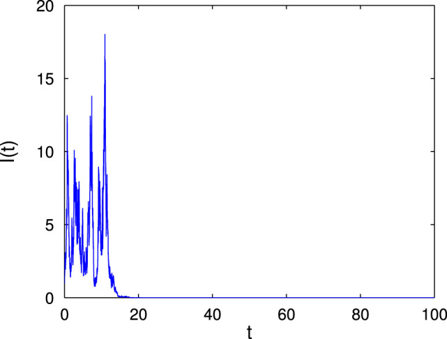
• 1. Large environment fluctuations can suppress the disease outbreak: Theorem 3.4 indicates that the extinction of disease in the stochastic model (4) occurs if the basic reproduction number ${\mathcal{R}}_0^s<1$. Theorem 2.1 shows that the deterministic model (2) admits a unique endemic equilibrium $E^{\ast }$ which is globally asymptotically stable if its basic reproduction number $R_0>1$. Notice that ${\mathcal{R}}_0^s=R_0-\frac{{\sigma }^2}{2(\mu +\gamma )}<R_0$, and hence there may exist a fact that ${\mathcal{R}}_0^s<1<R_0$. This is the case when the deterministic model (2) has an endemic (see Fig. 1) while the stochastic model (4) has disease extinction with probability one (see Fig. 4). This implies that large environment fluctuations under media coverage in $I$-class can suppress the outbreak of disease.
• 2. The stationary distribution exists in the case of ${\mathcal{R}}_0^s>1$: As suggested in Theorem 3.7, Remark 3.8 and Fig. 3, the stochastic model (4) has a stationary distribution if ${\mathcal{R}}_0^s>1$ (c.f., Fig. 3), which leads to the stochastic persistence of the disease.

Fig. 1.

The time-series plots of $S_t,I_t$ for the deterministic model (23) with initial $(S_0,I_0)=(5,1)$, and other parameters are taken as Table 1, $R_0=6.0>1$.

It isshould be pointed out that, although our SDE model (4) is similar to that in [2] (one incidence rate is bilinear, the other is standard [2]), the proving methods for stochastically disease dynamics are very different. In [2], the authors used the method of stochastic stability, and here, we use the Markov semigroup theory to prove stochastically asymptotic stability of model (4). On the other hand, in [2], the authors proved that if ${\mathcal{R}}_0^s<1$, under an extra conditions of $\sigma$, the disease goes to extinct with probability one (Theorem 3.1 in [2]); and in Theorem 3.4, we show that only when ${\mathcal{R}}_0^s<1$, does the disease die out almost surely, regardless of the intensity of environmental fluctuations $\sigma$. This point may show the different effect on the stochastic dynamics between the bilinear incidence rate with the standard incidence rate.

References

- 1.Cui J.A., Tao X., Zhu H. An SIS infection model incorporating media coverage. Rocky MT J. Math. 2008;38(5):1323–1334. [Google Scholar]
- 2.Cai Y., Kang Y., Banerjee M., Wang W.M. A stochastic epidemic model incorporating media coverage. Commun. Math. Sci. 2016;14(4):893–910. [Google Scholar]
- 3.Xiao D., Ruan S. Global analysis of an epidemic model with nonmonotone incidence rate. Math. Biosci. 2007;208(2):419–429. doi: 10.1016/j.mbs.2006.09.025. [DOI] [PMC free article] [PubMed] [Google Scholar]
- 4.Cai Y., Wang W.M. Fish-hook bifurcation branch in a spatial heterogeneous epidemic model with cross-diffusion. Nonlinear Anal. Real World Appl. 2016;30:99–125. [Google Scholar]
- 5.Cai Y., Kang Y., Banerjee M., Wang W.M. Complex dynamics of a host-parasite model with both horizontal and vertical transmissions in a spatial heterogeneous environment. Nonlinear Anal. Real World Appl. 2018;40:444–465. [Google Scholar]
- 6.Wang W.D., Ruan S. Simulating the SARS outbreak in Beijing with limited data. J. Theoret. Biol. 2004;227(3):369–379. doi: 10.1016/j.jtbi.2003.11.014. [DOI] [PMC free article] [PubMed] [Google Scholar]
- 7.Webb G., Blaser M., Zhu H., Ardal S., Wu J. Critical role of nosocomial transmission in the Toronto SARS outbreak. Math. Biosci. Eng. 2004;1(1):1–13. doi: 10.3934/mbe.2004.1.1. [DOI] [PubMed] [Google Scholar]
- 8.Liu R., Wu J., Zhu H. Media/psychological impact on multiple outbreaks of emerging infectious diseases. Comput. Math. Method. Med. 2007;8(3):153–164. [Google Scholar]
- 9.Øksendal B. Stochastic Differential Equations: An Introduction with Applications. sixth ed. Springer–Verlag Berlin Heidelberge; 2005. [Google Scholar]
- 10.Thomas C.G. Introduction to Stochastic Differential Equations. Marcel Dekker Inc.; New York: 1987. [Google Scholar]
- 11.Spencer S. Stochastic Epidemic Models for Emerging Diseases, Ph.D. Thesis. University of Nottingham; 2008. [Google Scholar]
- 12.Cai Y., Kang Y., Banerjee M., Wang W.M. A stochastic SIRS epidemic model with infectious force under intervention strategies. J. Differential Equations. 2015;259(12):7463–7502. [Google Scholar]
- 13.Truscott J.E., Gilligan C.A. Response of a deterministic epidemiological system to a stochastically varying environment. Proc. Natl. Acad. Sci. USA. 2003;100(15):9067–9072. doi: 10.1073/pnas.1436273100. [DOI] [PMC free article] [PubMed] [Google Scholar]
- 14.Rudnicki R. Long-time behaviour of a stochastic prey-predator model. Stochastic Process. Appl. 2003;108(1):93–107. [Google Scholar]
- 15.Wang W.M., Cai Y., Li J., Gui J. Periodic behavior in a FIV model with seasonality as well as environment fluctuations. J. Franklin Inst. B. 2017;354:7410–7418. [Google Scholar]
- 16.Lahrouz A., Settati A., Akharif A. Effects of stochastic perturbation on the SIS epidemic system. J. Math. Biol. 2016;74(1–2):469–498. doi: 10.1007/s00285-016-1033-1. [DOI] [PubMed] [Google Scholar]
- 17.Higham D.J. An algorithmic introduction to numerical simulation of stochastic differential equations. SIAM Rev. 2001;43(3):525–546. [Google Scholar]
- 18.Cai Y., Kang Y., Wang W.M. A stochastic SIRS epidemic model with nonlinear incidence rate. Appl. Math. Comput. 2017;305:221–240. [Google Scholar]
- 19.Wang W.M., Cai Y., Li J., Gui Z. Periodic behavior in a FIV model with seasonality as well as environment fluctuations. J Frank. Inst. 2017;354:7410–7428. [Google Scholar]
- 20.Mao X., Marion G., Renshaw E. Environmental Brownian noise suppresses explosions in population dynamics. Stochastic Process. Appl. 2002;97(1):95–110. [Google Scholar]
- 21.LaSalle J.P. The Stability of Dynamical Systems. Society for Industrial and Applied Mathematics; 1987. [Google Scholar]
- 22.Lyapunov A.M. The general problem of the stability of motion. Inter. J. Control. 1992;55(3):531–534. [Google Scholar]
- 23.Rudnicki R., Pichor K., Tyran-Kaminska M. Markov semigroups and their applications. Lecture Notes Phys. 2002;597:215–238. [Google Scholar]
- 24.Pichór K., Rudnicki R. Continuous Markov semigroups and stability of transport equations. J. Math. Anal. Appl. 2000;249(2):668–685. [Google Scholar]
- 25.Rudnicki R. On asymptotic stability and sweeping for Markov operators. Bull. Pol. Acad. Sci. Math. 1995;43:245–262. [Google Scholar]
- 26.Pichór K., Rudnicki R. Stability of Markov semigroups and applications to parabolic systems. J. Math. Anal. Appl. 1997;215(1):56–74. [Google Scholar]
- 27.Rudnicki R. Chaos — the Interplay Between Stochastic and Deterministic Behaviour. Springer Nature; 1995. Asymptotic properties of the Fokker–Planck equation; pp. 517–521. [Google Scholar]
- 28.Kadanoff L.P. Statistical Physics: Statics, Dynamics, and Renormalization. World Scientific; Singapore and New Jersey: 2000. [Google Scholar]
- 29.Stroock D.W., Varadhan S.R.S. Proceedings of the Sixth Berkeley Symposium on Mathematical Statistics and Probability, vol. 3. The University of California; 1970/1971. On the support of diffusion processes with applications to the strong maximum principle; pp. 333–359. [Google Scholar]
- 30.Ben Arous G., Lándre R. Dćroissance exponentielle du noyau de la chaleur sur la diagonale (II) Probab. Theor. Rel. 1991;90(3):377–402. [Google Scholar]
- 31.Liu Y., Cui J.A. The impact of media coverage on the dynamics of infectious disease. Int. J. Biomath. 2008;01(01):65–74. [Google Scholar]