

Abstract
This paper investigated the microparticle deposition and distribution due to the presence of duct bends by employing the Eulerian approach with Reynolds stress turbulent model and a Lagrangian trajectory method. The air velocity, particle velocity and particle deposition velocity were validated with available experimental data. Several particle deposition ratios were proposed to describe the particle accumulation due to bends. Particle deposition velocities in and behind bends were analyzed numerically. It is found that bend walls with surfaces of higher capture velocity tend to accumulate more contaminant particles as seen with an increased factor of 1.2 times on particle deposition velocity. Particle deposition reaches a maximum value near bend outlet, e.g. 15.2 times deposition ratio for particles of dp = 23 μm, and decay exponentially to a status of fully developed deposition in approximately 10D length. Compared to traditional consideration of sole deposition in bends, a new general concept of total deposition including that in bends and behind bends is proposed to better describe the particle deposition induced by bends since the enhancement deposition ratios behind bends compose 42–99% in the total ratios for particles of dp = 3–23 μm. Furthermore, models of fast power and exponential decay trend are demonstrated to uncover the relationship among enhancement factor of deposition velocity behind bend, dimensionless distance behind bends and particle Stokes number. The present study can contribute to the understanding and controlling of contaminant aerosol flow behavior in ducts, e.g. particle sampling, removal and associated epidemiologic study between particle and human health.
Keywords: Particle, Bend, Deposition ratio, Deposition velocity, Enhancement factor, New decay equation
Highlights
► Particles are easy to accumulation on walls with high capture velocity. ► Particle deposition has a peak value near bend outlet. ► Enhanced deposition behind bends is attributed to bend-induced turbulence. ► Deposition behind bends forms a large portion of the total bend-induced deposition. ► Exponential decay trend behind bends is found.
1. Introduction
Contaminant particles suspending in a room may cause health problems to the occupants [1], [2], [3], [4], [5], for example, robust associations between ambient PM concentrations and human morbidity and mortality [6] and the transmission of severe acute respiratory syndrome (SARS) [7]. Nowadays, to provide a comfortable built environment, central ventilation systems are commonly installed in modern commercial, institutional and public buildings, and therefore the ventilation ducts become one main way to transport particle-laden airflow [8]. In real ventilation ducts, one of the main parts is the bend for flow direction adjustment and pollutant aerosol deposition [9]. Additionally, there are other practical applications of particle flowing through bends, including the removal of particulates from industrial duct bends [10] and extractive sampling of pollutants in gas flow [11], [12].
To construct the ventilation ducts, many kinds of materials can be adopted [13], [14]. Several kinds of steel and aluminum with different coatings are used widely, and materials with special usage such as plastic, glass and masonry could also be found. Construction materials of ducts play significant roles in ventilation systems [13], [15]. In previous research, however, only Sippola and Nazaroff [16] investigated the deposition in 90° ventilation bends related to typical commercial or public mechanical ventilation systems. Peters and Leith [10] studied industrial pipe bends with grease coating which was assumed to capture all particles approaching it. In the reported studies of McFarland et al. [11] and Pui et al. [12], the deposition surface materials were not considered. Few research was conducted to investigate the particle distribution and deposition in 90° bends regarding different wall materials.
In view of the experimental approach, particle distribution and deposition are affected by many factors [17], [18], [19], hence the experimental analysis of the particle behavior throughout duct bends becomes quite challenging. The other method, computational fluid dynamics (CFD), has become an efficient and robust tool to investigate the airflow and particle behavior in ventilation ducts according to previous studies [20], [21], [22], [23]. However, little research adopted the CFD method including a discrete trajectory approach to study particle deposition and distribution throughout bends. In our previous studies [24], [25], the CFD approach together with an improved particle–wall impact model was successfully applied to predict the particle distribution and deposition in 90° bends.
Furthermore, experimental studies of the enhanced particle deposition behind bends have been reported recently [16], [26]. Miguel et al. [26] conducted the study of aerosol deposition and distribution in bifurcating duct system which corresponded to human respiratory system. It was found that particles accumulated mainly around the bend segment. Sippola and Nazaroff [16] investigated the mechanical ventilation system with bends and reported sharp increase of deposition velocity behind a bend about one to two order of magnitude. However, related research about the sole bend effect on the succeeding long straight duct was seldom found.
Therefore, this work aims to further study the particle deposition and distribution caused by bends by initiating the concept of deposition ratio and enhancement factor. The airflow phase and particle phase are solved by the Eulerian method with Reynolds Stress turbulent model and a Lagrangian discrete tracking approach with a particle–wall collision model, respectively. The improved CFD approach is then used to analyze the particle deposition ratio, deposition velocity and associated distributions inside and behind bends. In these perspectives, four demonstrating decaying equations are proposed to describe the enhanced deposition behind bends.
2. Research methods
2.1. Air phase model
The air phase which was governed by Eulerian conservation equations was predicted by employing the generic CFD approach, FLUENT [27]. The Reynolds stress model (RSM) was adopted to solve the airflow turbulence along with two-layer enhanced-wall model. This is attributed to the reason that this RSM model performs reasonably well for two-dimensional flows [28] because it accounts for the effects of curvature, swirl and rotation and can resolve the near-wall flow features. The ability of this model together with two-layer model has been verified clearly to prediction particle deposition in straight ducts accurately [29].
The flow boundary conditions were given as follows. At the flow outlet, Neumann boundary condition was adopted, i.e. mass conservation conditions for velocities and zero gradient boundary conditions for other variables. The duct walls were assumed to be smooth. In order to impose fully developed turbulence profile, the velocity profiles at flow inlet of y direction were defined according to the following 1/7th power law equations,
| (1) |
| (2) |
Where U ave is the averaged velocity in the straight duct before bend, D is the cross dimension accordingly and x D is nearest distance from one of the two inlet duct walls. The turbulent kinetic energy k was given as,
| (3) |
| (4) |
Where ρ a is the air density, the constant C 0 equals 0.09 and f is the fanning friction factor. This inlet condition was integrated into the CFD code by programming a user-defined function (UDF).
With regard to numerical scheme, the finite volume method (FVM) together with SIMPLE algorithm [30] was adopted within the CFD code. The RSM model employed the second-order upwind scheme for all the variables except pressure. The discretization of pressure was based on a staggered PRESTO! scheme [27]. Scaled convergent residuals were less than 10−5 for velocity components, turbulent quantities and Reynolds stress variables.
2.2. Particle phase model
The solid and spherical particle flow was assumed to be diluted enough to ignore the interaction of particle to particle and particle to air. Therefore, all the computational results were obtained by utilizing one-way coupling method. Depending on these assumptions [9], the Lagrangian formulations of particle motion were formed as follows,
| (5) |
Where u pi stands for particle velocity in the ith direction (m/s) and u i is the air velocity. The first term on the right is the drag forces exerted on the particle (per unit particle mass) in the ith direction (m/s2), and the second one is the gravitational force per unit particle mass. The third term means other potential forces. These forces were studied by Zhao et al. [22], and Saffman force was suggested to be important for large particles. Therefore, only this lift force was added into the third term of Eq. (5). Since the particle motion trajectory can be influenced by the instantaneous fluctuating airflow velocity, ‘Eddy lifetime’ model was utilized [31].
2.3. Particle–wall impact model
This particle–wall impact model initiated by Brach and Dunn [15] accounts for the particle–wall interaction including material dissipation, friction and adhesion in a convenient algebraic formula. The coefficient of restitution, e, can be written as follows,
| (6) |
Where, and are particle normal incident and reflected velocities, respectively, R pw for the coefficient of restitution without adhesion, ρ pw as the coefficient of adhesion. If this coefficient satisfies the relation ρ pw = 1, particles will be all trapped on a surface; if R pw equals 0, it means there is no adhesion effect. These two coefficients can be expressed as,
| (7) |
| (8) |
where, the parameters κ, l, a, b, and v c (capture/critical velocity) are determined by experimental method [15].
Due to the limited numbers of experimental surfaces, only three types of experimental surfaces were selected to analyze the material effect on particle deposition and distribution near the wall surfaces. These surface parameters are listed in Table 1 . The capture velocities for the three pairs of copper, mica and molybdenum surfaces are 0.29, 1.10 and 1.47 m/s respectively. It means that the particle motion near copper surface possesses the lowest capture velocity and that near molybdenum hold the highest. The particles are assumed to be captured on a surface if the incident normal velocity falls below the capture velocity. To incorporate the particle–wall impact model into the CFD code, a UDF program in bends was developed.
Table 1.
Condition and information for example particle impacts [15].
| Particle diameter (μm) | Particle material | Surface material | k | l | a | b | νc (m/s) |
|---|---|---|---|---|---|---|---|
| 8.6 [1–30] | Ag-coated glass | Copper | 38.7 | 1.61 | 1.0 | 1.0 | 0.29 |
| 3–7 | Ammonium fluorescein | Mica | 72.5 | 1.333 | 1.0 | 1.0 | 1.10 |
| Ammonium fluorescein | Molybdenum | 55.7 | 0.586 | 1.0 | 1.0 | 1.47 |
Three particle size groups (3, 5 and 7 μm) were studied with three different surface materials to conduct material comparisons considering the available narrow range (3–7 μm) of particle diameter provided by existing experimental data [15]. For copper surface, another four particle sizes (10, 16, 20 and 23 μm) were also investigated to estimate the particle deposition velocity, and to compare the prediction result with available experimental data.
2.4. Particle deposition analysis in bends
This study presented the following two methods for the investigation of the particle deposition results in bends:
-
1)
By demonstrating the particle deposition amount at different reflection angle from θ = 0° to 90°. The deposited particle number N dθ from the bend entrance to a specific angle θ was expressed as,
| (9) |
Where N 0 and N θ are the particle number traveling through bend entrance and reflection angle , respectively.
In order to interpret the deposition amount increase caused by bend, a concept of “bend-induced deposition ratio throughout a bend” (R db) was proposed as follows,
| (10) |
Where N d and N f are the particle number deposited in a bend and those in the straight duct of fully developed flow section with a length D, respectively. In this article, N f is selected as the average deposited particles between the reference sections of 3D–2D and 2D–1D before bend inlet. R b and D are bend radius and the cross dimension of the straight duct before bend, respectively. The symbol α stands for the total reflection angle of the bend, and in this paper it is π/2. In this formula, the deposition in the bend is treated as “equivalent length of straight duct” with fully developed flow. This deposition ratio can show the average deposition amount enhancement due to bend-induce flow turbulence and direction change.
-
1)
By employing the correlation between dimensionless particle deposition velocity and particle relaxation time , which are determined by the following equations,
| (11) |
| (12) |
where, V d means the deposition velocity, u w is the friction velocity, C c is the Cunningham slip correction factor, ρ p stands for the particle density, d p is the particle diameter, μ and ν are dynamic and kinematic viscosity respectively of air. In this proposed Lagrangian tracking approach, the particle deposition velocity onto a bend surface can be generally estimated by calculating the number of deposited trajectories in a time period as below,
| (13) |
where, t b is the flying time scale for particles through a bend; N 0 and N d are the numbers respectively of the particles that enter the entrance of the bend and those deposited within the bend; and, A and V are the area and volume of deposition bend respectively. Similar method to Eq. (13) has been successfully employed before by previous researchers [18], [32] to predict particle deposition in straight duct flow.
2.5. Particle deposition analysis behind bends
To investigate bend-induced particle deposition behind bends, this paper gives two methods as follows:
-
1)
By adopting the relationship between dimensionless particle deposition velocity and dimensionless particle relaxation time , which has been expressed in Eqs. (11), (12). The particle deposition velocity V da behind bends was estimated by the following equation,
| (14) |
Where u b stands for the bulk flow velocity at the domain inlet, N in is the particle number entered into a specific straight duct section, N out is the particle number escaped from the straight duct section, D is the duct cross dimension, L is the length of the straight duct. This approach has been proved before in sole straight duct particle deposition [9], and it is applied here to study the deposition behind bends with developing turbulence [16]. The enhancement factor of deposition velocity behind bends (e da) can be calculated by,
| (15) |
Where V df is the deposition velocity in straight duct between the reference sections of 3D–2D and 2D–1D before bend inlet, where the flow is assumed to be fully developed. This deposition velocity is also estimated by Eq. (14).
-
2)
By introducing a concept of “bend-induced deposition ratio behind a bend” (R da) as follows,
| (16) |
Where N da is the deposited particle number behind a bend at a specific straight duct section. Following this expression, the increased degree and trend of particle deposition can be clearly seen due to the bend-induced turbulence behind the bend.
Combining Eq. (10) and Eq. (16), “total bend-induced deposition ratio per cross dimension D” (R dt) can be expressed as,
| (17) |
Where s is the distance away from bend outlet. This equation reflects the total particle deposition amount increase due to bend.
Furthermore, relatively to the deposition in fully developed flow section, “total bend-induced enhancement deposition ratio per cross dimension D” (R dte) can be determined by subtracting the deposition of fully developed section in the equation above,
| (18) |
This definition shows the total ratio of the additional deposition increase attributed to the existence of bend.
3. Results and discussion
3.1. Numerical domain and mesh
The geometry and mesh of a two-dimensional 90° bend are shown in Fig. 1 . With regard to this bend, the width D, radius R b and curvature ratio R o are 0.1 m, 0.17 m and 3.4, respectively. Four grid systems were tested to check the mesh independence as shown in Table 2 . All the grids were denser near the wall areas to solve boundary flows with the first near-wall grid from 0.0044 to 4.2 for the four grid systems. The mesh numbers in bends were respectively 42 000, 15 400, 9744 and 5850 from grid system 1 to 4 as stated in Table 2. The results in Fig. 2 show similar results are obtained from the different grid systems with 97% agreement. Therefore, a relatively coarser grid system, i.e. system 3, was chosen to benefit the computational efficiency.
Fig. 1.

Two-dimensional 90° bends geometry and mesh.
Table 2.
Characteristics of the four grid systems for mesh independence test.
| Grid system | Total mesh no. | Mesh no. before bend | Mesh no. in bend | Mesh no. behind bend |
|---|---|---|---|---|
| System 1 | 240 000 | 120 × 750 | 120 × 350 | 120 × 900 |
| System 2 | 85 400 | 70 × 460 | 70 × 220 | 70 × 540 |
| System 3 | 57 884 | 58 × 380 | 58 × 168 | 58 × 450 |
| System 4 | 31 500 | 45 × 270 | 45 × 130 | 45 × 300 |
Fig. 2.

Comparison of air velocity profile at bend inlet at four grid systems.
3.2. Numerical validation
Sixty thousand monodisperse spherical particles uniformly distributed at the entrance of the computational domain were released as Lagrangian discrete tracking approach was employed to solve the particle motion equation. The influence of this particle number on particle motion was checked with two hundred thousand particles, and subtle difference was found. In addition, the densities of the particles and the air are 2990 kg/m3 and 1.225 kg/m3, respectively. The air viscosity is 1.7894 × 10⁻⁵ kg/m/s.
Present simulation results are shown together with previous results of laser Doppler velocimetry (LDV) experiment [33] in Fig. 3, Fig. 4 . The air and particle velocities were normalized by the bulk air velocity u b, and these dimensionless velocities were plotted against dimensionless wall distance r∗ for comparison as shown in Fig. 1. The comparisons indicate that the present model achieve more than 95% consistency with experimental data. This result shows that two-dimensional flow is accurate enough and relatively efficient. Since current numerical study focuses on introducing and studying the concept of bend-induced deposition in and behind bends, therefore, the simplified two-dimensional bend is utilized in this article.
Fig. 3.

Comparison of air velocity profile with experimental data in the bend at θ = 0° and 15°.
Fig. 4.

Comparison of particle velocity profile with experimental data in the bend at θ = 0° and 15°.
3.3. Particle deposition distribution with three surface materials in bends
Fig. 5 demonstrates the detailed particle numbers deposited from bend inlet to locations at the four deflection section θ = 0°–90° with three surfaces for d p = 3–7 μm particles. The deposited particles are calculated by Eq. (9). The deposition particle number increases slowly from θ = 0° to 60° and obviously from θ = 60°–90°. When particle diameter d p increase from 3 μm to 7 μm, the particle number at the bend entrance decreases considerably, especially for molybdenum surfaces. With much larger particles in the experimental parameters, this decreased degree would be much higher, especially for large capture velocity surfaces. Take d p = 7 μm for example, the deposited particles in bends are 1.7 times on molybdenum surfaces to those on copper surfaces.
Fig. 5.

Comparison of deposited particle number before locations of θ = 0°–90° with three surfaces: (a) dp = 3 μm; (b) dp = 5 μm; (c) dp = 7 μm.
3.4. Particle deposition velocity with three surface materials in bends
Fig. 6 summarizes previous experimental data and predicted particle deposition velocities against particle relaxation time in 90° bends. The average particle deposition velocities were calculated through control volume method by Eqs. (11), (12), (13) for d p = 3–16 μm particles. To validate and compare the simulated results, three typical experiments [11], [12], [16] in 90° bends were collected in the figure. The experimental data from Liu & Agarwal [34] was also presented to compare the deposition velocities in bends with those in straight ducts.
Fig. 6.

Comparison of average particle deposition velocity with experimental data in 90° bends with copper surface for dp = 3–16 μm particles.
It can be seen that predicted deposition velocities in bends are much larger than those in straight ducts by one or two orders of magnitude. Sippola and Nazaroff [16] also drew a similar conclusion when comparing their experimental data in bends with those in their straight ducts. Among the three experiments in bends, result data also change by about one order of magnitude due to different experimental conditions. Simulated particle deposition velocities from = 1.2 to 32.9 fall within the experimental data [11], [12], [16].
The surface effect on particle deposition velocity can be clearly seen from Fig. 7 . The deposition velocity with copper surface is the lowest. This observation can also be seen in Fig. 5 where deposited particle numbers with different surfaces are presented. The reason of a low deposition velocity with copper surface could be due to the low capture velocity near such surface. Between particle relaxation time , the particle deposition velocity with molybdenum surface is 0.7–1.2 times larger than that of a copper surface. Given more experimental data about particle collision behavior onto different surfaces with a wide particle diameter range, more deposition velocities could be predicted following the proposed method in this work.
Fig. 7.

Comparison of average particle deposition velocity in 90° bends with three surfaces for dp = 3–7 μm particles.
3.5. Particle deposition velocity behind bends
Since a bend in the flow stream can cause the change of flow pattern and lead to flow turbulence behind bends, the particle deposition behind bends would be enhanced due to the bend. To describe the deposition change along the straight duct behind a bend, dimensionless distance (s∗) is expressed as s∗ = (La − x)/D, which is shown in Fig. 8 . In the present work, the dimensionless distance is an integer number. In the equation, La is the total straight duct length behind bends, which equals 1.2 m in this paper, and x is the horizontal coordinate. In addition, the predicted results in the following discussion were simulated based on the wall surfaces of the lowest capture velocity.
Fig. 8.
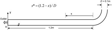
Dimensionless distance behind bend, s∗.
Fig. 9 shows the comparison of average particle deposition velocity behind 90° bends for d p = 3–23 μm particles from s∗ = 1 to 12. Correspondingly, the Stokes numbers of these particles are from 0.016 to 0.89. Each particle deposition velocity at an s∗ value is the average deposition velocity based on the deposition particle numbers from s∗ − 1 to s∗. The calculation method can be found in Eq. (14). As shown in the figure, the magnitude of the dimensionless particle deposition velocity changes from 0.0317 to 1.332, which is much higher than those illustrated in Fig. 6, Fig. 7. This behavior provides quantitative evidence through simulation that the deposition behind the bend is enhanced due to bend-induced turbulence. Along with the increasing of dimensionless particle relaxation time from , the deposition velocity increases sharply by 4.8–10 times. Current results of the enhanced particle deposition behind bends and the changing trend could explain and support previous experimental visualized observations and reports behind bends qualitatively [16], [26].
Fig. 9.
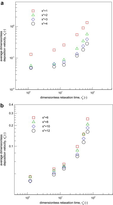
Comparison of average particle deposition velocity behind bends for dp = 3–23 μm particles from s∗ = 1 to 12.
However, when the distance increases away from the bend outlet, i.e. from s∗ = 1 to 12, the particle deposition velocity decrease. The maximum deposition velocity is located at s∗ = 1, which means the areas between bend outlet and one cross dimension distance for particles of specific Stokes number. From s∗ = 1 to 2, the particle deposition velocity reduces tremendously, which reflects the rapidly decreasing influence of bend-induced vortices. The reduction degree from s∗ = 2 to 5 is moderate and from s∗ = 6 to 12 is minor. The decreasing deposition could be probably attributed to the turbulent level reduction when the distance increase behind bends as shown in Fig. 10 . From s∗ = 1 to 5, it can be seen in the figure that large vortices are produced behind the bend, while from s∗ = 6 to 12, turbulent levels are rather low.
Fig. 10.

Turbulent kinetic energy of the airflow in and behind bends.
3.6. Bend-induced deposition ratio
To describe the quantity of particle deposition along the straight duct behind bends, the bend-induced deposition parameter Rda is demonstrated in Fig. 11 . In the presentations of the deposition ratio and the following enhancement factor, Eqs. (1), (2), (3), (4) were adopted at the domain inlet to guarantee the airflow was fully developed in straight duct ahead of bends. The results range from R da = 0.91 to 15.2, which indicate the quantitative increase of particle deposition caused by bend. Particle accumulation is very high near the bend outlet. Deposition ratios increase from 4.61 to 15.2 times for particle diameters increasing from d p = 3–23 μm. The deposition is reduced sharply from areas near the bend outlet to those further away from it. From s∗ = 10 to 12, the deposition ratios are close to unity 1. This phenomena means that the flow disturbance due to bend is weakened to a marginal level at these areas, and the length of increased deposition due to the presence of the bend is 10 times as long as the cross dimension (D) of straight duct. This interpretation is partially supported by the experimental measurements of particle deposition in developing turbulent flow in the studies of Sippola and Nazaroff [16].
Fig. 11.

Bend-induced deposition ratio distribution along the distance behind bend for different particle diameter.
Fig. 12 illustrates the bend-induced enhancement deposition ratio in and behind bends for present simulation domain. The enhancement deposition ratios in bends and behind bends correspond to the first and second term in Eq. (18), respectively. These ratios are calculated based on Eqs. (16), (17), (18). They can be also called as additional deposition caused by bend. For small particles, for example, d p = 3 μm, the enhancement deposition ratio is rather low because the ratio considers the bend as equivalent straight duct and the Stokes number indicates that small particles are easy to follow fluid flow. In other words, smaller particles are hardly to impact onto bend walls. However, the flow pattern change by bends also leads to deposition enhancement behind bends, and the total ratio is mainly composed of the enhancement deposition behind bends, approximately 99% for particles of d p = 3 μm. This behavior is probably due to that eddies behind bends are adaptable to catch smaller particles onto wall surfaces as demonstrated in Fig. 12. For larger particles, the major composition of the total ratio is reversed, i.e. in bends. However, the deposition behind bends are still of a great portion, approximately 42% for particles of d p = 23 μm. Therefore, when describing the particle deposition induced by bends, the general concept of total deposition including that in bends and behind bends is much better than sole particle accumulation in bends.
Fig. 12.

Bend-induced enhancement deposition ratio for six particle diameters.
3.7. Changing trend of bend-induced deposition ratio
It is interesting to find that the decay trend of particle deposition ratio behind bend in Fig. 11. This decay trend satisfies two conditions: (1) it peaks at s∗ = 1; (2) when s∗ ≥ ∞, the deposition ratio asymptotically approaches unity 1. The second condition means the particle deposition is in a fully developed flow. Therefore, subtracting the deposition in a fully developed flow, the “enhancement deposition ratio behind a bend” (R dae) would be infinitely small at s∗ ≥ ∞. Take the particles of d p = 20 μm for example, as shown in Fig. 13 , the relationship between the enhancement deposition ratio (R dae) and dimensionless distance (s∗) can be built as follows,
| (19) |
Fig. 13.

Bend-induced enhancement deposition ratio behind bend for dp = 20 μm particles.
The R 2 value is as high as 0.982, which shows a well-fitting between the simulation data and the proposed equation. In addition, this fitting can also transformed as exponential correlation between the two variables. For other particle diameters, similar fittings can be obtained through this method.
3.8. Changing trend of enhancement deposition ratio
Enhancement factor of deposition velocity behind a bend (e da) varies with dimensionless distance (s∗) and particle diameter or Stokes number (St), as shown in Fig. 11. A three-dimensional surface fitting code (TableCurve 3D, Jandel Scientific, San Rafael, CA) was adopted to develop least square fits of the current simulation data [11]. Therefore, a non-linear fitting of R 2 = 0.994 could be expressed as follows,
| (20) |
Where x s∗ is the lognormal distribution function with s∗ and stands for the Gaussian distribution function with St, as shown in Fig. 14 . The enhancement deposition ratio has exponential decreasing relationship only with dimensionless distance and particle Stokes number. This relationship is valid for s∗ = 1–12 and St = 0.016–0.89.
Fig. 14.

Enhancement factor of particle deposition velocity behind bend for dp = 3–23 μm particles.
3.9. Changing trend of dimensionless deposition velocity behind bend
Combining Eq. (15) and Eq. (20), the dimensionless deposition velocity behind bend is deducted as,
| (21) |
Which means the dimensionless deposition velocity in the developing turbulent flow behind bend can be associated with the reference dimensionless deposition velocity by the enhancement factor. Substituting the dimensionless parameter St with , the function y St becomes,
| (22) |
This equation reveals that the dimensionless deposition velocity behind bend () is related to dimensionless particle relaxation time as shown in Fig. 9.
Furthermore, the curves of s∗ = 6–12 shown in Fig. 9 exhibit similarity to develop a more universal relationship than that in Eq. (21). By averaging seven dimensionless deposition velocities at each dimensionless relaxation time, Fig. 15 is obtained together with the standard deviation of the averaged values. Using a polynomial fitting of R 2 = 0.999, the relationship is expressed as,
| (23) |
Fig. 15.

Fitting curve of dimensionless deposition velocity averaged from s∗ = 6 to 12 behind bends for dp = 3–23 μm particles.
Under current simulation conditions, this relationship reveals that dimensionless deposition velocity depends only on dimensionless relaxation time for s∗ = 6–12 as demonstrated in Fig. 15. Therefore, Eq. (23) is easy to use in the applications.
4. Conclusions
This paper investigated the microparticle deposition in and behind 90° bends. Particle deposition distribution and deposition velocity in 90° ventilation bends with different surface materials were analyzed numerically, and the simulation results were also validated with experimental data. Bend-induced deposition ratio and deposition velocity were also discussed and fitted quantitatively. To summarize, the following conclusions can be drawn:
-
a)
Predicted particle deposition velocities in bends are much higher than those in straight ducts by one to two orders of magnitude. Between the predicted particle relaxation time 1.2 and 6.4, the particle deposition velocities with surfaces of highest capture velocity can be 1.2 times larger than those of lowest capture velocity. This behavior indicates that the duct bend wall with surfaces of high capture velocity is easy to accumulate contaminant particles.
-
b)
Current simulation provided quantitative evidence that the deposition behind a bend is sharply enhanced due to bend-induced turbulence. Particle deposition had a peak value near bend outlet. Along the straight duct behind bends, the depositions decreased exponentially toward a deposition pattern of fully developed turbulent flow since the bend-induced eddies are weakened.
-
c)
It is much better to adopt the general concept of total deposition including that in bends and behind bends to describe the particle deposition induced by bends. Deposition behind bends forms a large portion of the total bend-induced deposition, especially for smaller particles.
-
d)
Power decay trend was obtained between the enhancement deposition ratio (R dae) and dimensionless distance (s∗). Non-linear exponential decay trend was also given among enhancement factor of deposition velocity behind a bend (e da), dimensionless distance (s∗) and particle Stokes number (St). These fitting equations are valid according to the current simulation condition for the ranges of s∗ = 1–12 and St = 0.016–0.89. Finally, two fitting equations of dimensionless deposition velocity behind bend were developed to model the deposition trend easily and universally.
This work proposed new concepts of bend-induced deposition which includes the deposition both in bends and behind bends. Quantitative discussion was given to evaluate the two location depositions. The decaying correlations were proposed based on current results. This paper contributes to the understanding of pollutant particle deposition and distribution in and behind ventilation duct bends, which can be applied on contaminant particle sampling, removal and associated epidemiologic study between particle and human health through ventilation system.
Acknowledgment
This work was financially supported by the Hong Kong Polytechnic University through research grants A-PJ61 and A-PJ12.
Nomenclature
- A
area of deposition, m2
- C0
constant in Eq. (3)
- Cc
Cunningham slip correction factor
- dp
particle diameter, m
- D
bend width or cross dimension of straight duct, m
- e
kinematic restitution coefficient
- eda
enhancement factor of deposition velocity behind a bend
- f
fanning factor
- gi
gravity acceleration, ms−2
- l,a,b
- L
length of the straight duct behind a bend, m
- La
total length of the straight duct behind a bend, m
- k
turbulent kinetic energy, kg ms−1
- N0
number of particles flew across bend entrance
- Nd
number of particles deposited on bend wall surface
- Nda
number of particles deposited behind a bend at a specific straight duct section
- Nf
number of particles deposited on straight duct of fully developed flow section ahead of a bend
- Nin
number of particles entered into a specific straight duct section behind a bend
- Nout
number of particles escaped from a specific straight duct section behind a bend
- Nθ
number of particles flew across bend reflection angle
- r1, r2
radius of the inner and outer wall of the bend, respectively, m
- r∗
dimensionless wall distance
- Ro
bend curvature ratio
- Rb
bend radius, m
- Rda
bend-induced deposition ratio behind a bend
- Rdae
bend-induced enhancement deposition ratio behind a bend
- Rdb
bend-induced deposition ratio throughout a bend
- Rdt
total bend-induced deposition ratio per cross dimension D
- Rdte
total bend-induced enhancement deposition ratio per cross dimension D
- Rpw
coefficient of restitution in the absence of adhesion
- t
time, s
- s
distance behind bend outlet, m
- s∗
dimensionless distance behind bend outlet, integer in this paper
- St
Stokes number
- tb
flying time scale for particles through a bend, s
- ub
air bulk velocity, ms−1
- ua,U
air velocity, ms−1
- up, upi
particle velocity, ms−1
- uw
friction velocity, ms−1
- vc
capture velocity, ms−1
- ,
particle normal incident and reflected velocity, respectively, ms−1
- V
volume of the domain, m3
- Vd
deposition velocity, ms−1
- Vda
deposition velocity in straight duct behind a bend, ms−1
- Vdf
deposition velocity in straight duct of fully developed flow section ahead of a bend, ms−1
dimensionless deposition velocity
- xD
horizontal coordinate, m
- xs∗
lognormal distribution function with s∗
- y
vertical coordinate, m
- ySt
Gaussian distribution function with St
Greek symbols
- α
total reflection angle of the bend, i.e. here π/2
- k
empirical constant in Eq. (7)
- μ
dynamic viscosity of air, Pa s
- ν
kinematic viscosity of air, m2 s−1
- ρa
air density, kg m−3
- ρp
particle density, kg m−3
- ρpw
adhesion coefficient
- θ
deflection angle
dimensionless particle relaxation time
References
- 1.WHO . World Health Organization; Geneva, Switzerland: 2006. Air quality guidelines for particulate matter, ozone, nitrogen, dioxide and sulfur dioxide. Global Update 2005, Summary of Risk Assessment. [PubMed] [Google Scholar]
- 2.Jin H.H., Fan J.R., Zeng M.J., Cen K.F. Large eddy simulation of inhaled particle deposition within the human upper respiratory tract. Aerosol Sci. 2007;38:257–268. [Google Scholar]
- 3.Gao N.P., Niu J.L. Modeling particle dispersion and deposition in indoor environments. Atmos Environ. 2007;41:3862–3876. doi: 10.1016/j.atmosenv.2007.01.016. [DOI] [PMC free article] [PubMed] [Google Scholar]
- 4.Chao C.Y.H., Wan M.P., Morawska L., Johnson G.R., Ristovski Z.D., Hargreaves M. Characterization of expiration air jets and droplet size distributions immediately at the mouth opening. Aerosol Sci. 2009;40:122–133. doi: 10.1016/j.jaerosci.2008.10.003. [DOI] [PMC free article] [PubMed] [Google Scholar]
- 5.Yu M.Z., Lin J.Z. Nanoparticle-laden flows via moment method: a review. Int J Multiph Flow. 2010;36:144–151. [Google Scholar]
- 6.Pope C.A., Dockery D.W. Epidemiology of particle effects. In: Holgate S.T., Samet J.M., Koren H.S., Maynard R.L., editors. Air pollution and health. Academic Press; London: 1999. pp. 673–705. [Google Scholar]
- 7.Knight J. Researchers get to grips with cause of pneumonia epidemic. Nature. 2003;422:547–548. doi: 10.1038/422547a. [DOI] [PMC free article] [PubMed] [Google Scholar]
- 8.Li Y., Leung G.M., Tang J.W., Yang X., Chao C.Y.H., Lin J.Z. Role of ventilation in airborne transmission of infectious agents in the built environment – a multidisciplinary systematic review. Indoor Air. 2007;17:2–18. doi: 10.1111/j.1600-0668.2006.00445.x. [DOI] [PubMed] [Google Scholar]
- 9.Zhang J.P., Li A.G., Li D.S. Modeling deposition of particles in typical horizontal ventilation duct flows. Energ Convers Manage. 2008;49:3672–3683. [Google Scholar]
- 10.Peters T.M., Leith D. Particle deposition in industrial duct bends. Ann Occup Hyg. 2004;48:483–490. doi: 10.1093/annhyg/meh031. [DOI] [PubMed] [Google Scholar]
- 11.McFarland A.R., Gong H., Muyshondt A., Wente W.B., Anand N.K. Aerosol deposition in bends with turbulent flow. Environ Sci Technol. 1997;31:3371–3377. [Google Scholar]
- 12.Pui D.Y.H., Romaynovas F., Liu B.Y.H. Experimental study of particle deposition in bends of circular cross-section. Aerosol Sci Technol. 1987;7:301–315. [Google Scholar]
- 13.ASHRAE Inc . American Society of Heating, Refrigerating and Air-Conditioning Engineers, Inc.; 2008. ASHRAE handbook – heating, ventilating, and air-conditioning systems and equipment (I-P Edition) [Google Scholar]
- 14.Sippola M.R. University of California; Berkeley, California: 2002. Particle deposition in ventilation ducts. [Google Scholar]
- 15.Brach R.M., Dunn P.F. Models of rebound and capture for oblique microparticle impacts. Aerosol Sci Technol. 1998;29:379–388. [Google Scholar]
- 16.Sippola M.R., Nazaroff W.W. Particle deposition in ventilation ducts: connectors, bends and developing turbulent flow. Aerosol Sci Technol. 2005;39:139–150. [Google Scholar]
- 17.Lin J.Z., Lin P.F., Chen H.J. Research on the transport and deposition of nanoparticles in a rotating curved pipe. Phys Fluids. 2009:21. [Google Scholar]
- 18.Zhang Z., Chen Q. Prediction of particle deposition onto indoor surfaces by CFD with a modified Lagrangian method. Atmos Environ. 2009;43:319–328. [Google Scholar]
- 19.Zhao B., Wu J. Particle deposition in indoor environments: analysis of influencing factors. J Hazard Mater. 2007;147:439–448. doi: 10.1016/j.jhazmat.2007.01.032. [DOI] [PubMed] [Google Scholar]
- 20.Chen Q. Comparison of different k-epsilon models for indoor air-flow computations. Numer Heat Tr B Fund. 1995;28:353–369. [Google Scholar]
- 21.Lai A.C.K., Chen F.Z. Modeling particle deposition and distribution in a chamber with a two-equation Reynolds-averaged Navier–Stokes model. Aerosol Sci. 2006;37:1770–1780. [Google Scholar]
- 22.Zhao B., Zhang Y., Li X.T., Yang X.D., Huang D.T. Comparison of indoor aerosol particle concentration and deposition in different ventilated rooms by numerical method. Build Environ. 2004;39:1–8. [Google Scholar]
- 23.Tu J.Y., Yeoh G.H., Morsi Y.S., Yang W. A study of particle rebounding characteristics of a gas-particle flow over a curved wall surface. Aerosol Sci Technol. 2004;38:739–755. [Google Scholar]
- 24.Sun K., Lu L., Jiang H. A computational investigation of particle distribution and deposition in a 90° bend incorporating a particle–wall model. Build Environ. 2011;46:1251–1262. [Google Scholar]
- 25.Jiang H., Lu L., Sun K. Experimental study and numerical investigation of particle penetration and deposition in 90 degrees bent ventilation ducts. Build Environ. 2011;46:2195–2202. [Google Scholar]
- 26.Miguel A.F., Reis A.H., Aydin M. Aerosol particle deposition and distribution in bifurcating ventilation ducts. J Hazard Mater. 2004;116:249–255. doi: 10.1016/j.jhazmat.2004.09.013. [DOI] [PubMed] [Google Scholar]
- 27.ANSYS Inc . 2010. ANSYS FLUENT 12.0 users guide. Lebanon, NH. [Google Scholar]
- 28.Zhang Z., Zhai Z.Q., Zhang W., Chen Q.Y. Evaluation of various turbulence models in predicting airflow and turbulence in enclosed environments by CFD: part 2-comparison with experimental data from literature. HVAC&R Res. 2007;13:871–886. [Google Scholar]
- 29.Tian L., Ahmadi G. Particle deposition in turbulent duct flows – comparisons of different model predictions. Aerosol Sci. 2007;38:377–397. [Google Scholar]
- 30.Partankar S.V. Hemisphere; Washington, DC: 1980. Numerical heat transfer and fluid flow. [Google Scholar]
- 31.Graham D.I., James P.W. Turbulent dispersion of particles using eddy interaction models. Int J Multiph Flow. 1996;22:157–175. [Google Scholar]
- 32.Zhang H.F., Ahmadi G. Aerosol particle transport and deposition in vertical and horizontal turbulent duct flows. J Fluid Mech. 2000;406:55–80. [Google Scholar]
- 33.Kliafas Y., Holt M. LDV measurements of a turbulent air-solid 2-phase flow in a 90-degree bend. Exp Fluids. 1987;5:73–85. [Google Scholar]
- 34.Liu B.Y.H., Agarwal J.K. Experimental observation of aerosol deposition in turbulent flow. Aerosol Sci. 1974;5:145–148. IN1–IN2, 9-55. [Google Scholar]