The daily computed weighted averaging basic reproduction number $R_{0,k,\omega }^n$ for MERS-CoV in South Korea

Abstract

In this paper, we propose the daily computed weighted averaging basic reproduction number $R_{0,k,\omega }^n$ for Middle East respiratory syndrome coronavirus (MERS-CoV) outbreak in South Korea, May to July 2015. We use an SIR model with piecewise constant parameters $\beta$ (contact rate) and $\gamma$ (removed rate). We use the explicit Euler’s method for the solution of the SIR model and a nonlinear least-square fitting procedure for finding the best parameters. In $R_{0,k,\omega }^n$, the parameters $n$, $k$, and $w$ denote days from a reference date, the number of days in averaging, and a weighting factor, respectively. We perform a series of numerical experiments and compare the results with the real-world data. In particular, using the predicted reproduction number based on the previous two consecutive reproduction numbers, we can predict the future behavior of the reproduction number.

1. Introduction

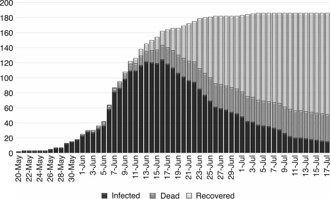
Middle East respiratory syndrome coronavirus (MERS-CoV), first identified in Saudi Arabia in June 2012, is a viral respiratory disease caused by a novel coronavirus  [1]. South Korea experienced the largest outbreak of MERS-CoV infections outside the Arabian peninsula  [2]. There have been 186 confirmed infective cases in South Korea within two months after the first infective person who returned from a trip to the Arabian peninsula was diagnosed on 11 May, 2015, and 38 people died and more than 16,000 people were quarantined due to the spread of the disease. Fig. 1 represents the epidemic curve of MERS-CoV, South Korea, 20 May–17 July 2015  [3], [4].

Fig. 1.

Epidemic curve of MERS-CoV, South Korea, 20 May–17 July 2015.

In order to implement appropriate surveillance and control measures, it is very important to predict the future trend of the epidemic. Therefore, it is the purpose of the present paper to show daily computed reproduction numbers for epidemics, in particular, MERS-CoV, so that we can predict the future behavior of the reproduction number day-by-day.

In the mathematical modeling of the spread of an epidemic disease, it is crucial to estimate the parameters (e.g., contact rate and recovery rate in an SIR model), but it is difficult to do so due to the lack of data available for the estimation. In case of the MERS-CoV spread in South Korea, there are almost complete daily data of the spread of the disease, and we choose the MERS-CoV spread case in South Korea as an epidemic model to verify the validity and accuracy of the method proposed in this paper. To the authors’ knowledge, there have been no previous works that present computational methods for estimation of the values of the epidemic parameters based on actual daily epidemic data.

The rest of the paper is organized as follows. In Section  2, we describe the mathematical model. In Section  3, we provide a numerical algorithm for the estimation of the parameters. We perform several numerical experiments in Section  4. In Section  5, we provide a summary and present our conclusions.

2. The mathematical model

In this paper, we consider the SIR model that was introduced in 1927 by A.G. McKendrick and W.O. Kermack  [5]. The model is simple and has been widely used so far, for instance, in multigroup epidemic modeling  [6], online social network dynamics  [7], the model adopting the delay term  [8], stochastic model  [6], [9], [10], vaccination strategy  [11], [12]. In this model, the population is divided into susceptible $S\left(t\right)$, infected $I\left(t\right)$, and removed $R\left(t\right)$ individuals at time $t$. The governing ordinary differential equations for the SIR model are as follows:

$$\frac{dS\left(t\right)}{dt}=-\beta S\left(t\right)I\left(t\right)\text{,}$$ (1)

$$\frac{dI\left(t\right)}{dt}=\beta S\left(t\right)I\left(t\right)-\gamma I\left(t\right)\text{,}$$ (2)

$$\frac{dR\left(t\right)}{dt}=\gamma I\left(t\right)$$ (3)

with initial condition $S\left(0\right)=S^0$, $I\left(0\right)=I^0$, and $R\left(0\right)=R^0$. Here, the parameters $\beta$ and $\gamma$ denote the contact (susceptibility to disease) and removed (either dead or recovered) rates from disease, respectively  [13]. We assume that a removed individual can never be infected again. Let $N$ be the constant total population size. Therefore, it is sufficient to solve only two Eqs. (1), (2), i.e., $R\left(t\right)=N-S\left(t\right)-I\left(t\right)$. By assuming that $\beta$ and $\gamma$ are time-dependent parameters, we generalize Eqs. (1), (2), (3) as follows:

$$\frac{dS\left(t\right)}{dt}=-\beta \left(t\right)S\left(t\right)I\left(t\right)\text{,}$$ (4)

$$\frac{dI\left(t\right)}{dt}=\beta \left(t\right)S\left(t\right)I\left(t\right)-\gamma \left(t\right)I\left(t\right)\text{,}$$ (5)

$$\frac{dR\left(t\right)}{dt}=\gamma \left(t\right)I\left(t\right)\text{.}$$ (6)

For example, the transmission of the vector-borne diseases such as Dengue fever and Malaria has strong seasonal patterns and thus the parameters are estimated as the time-dependent functions  [14], [15]. Another example is a seasonal SIR model for the spread of the whooping cough in which the contact rate $\beta$ is given as a time-dependent periodic function which accounts seasonal changes  [16].

3. The numerical method

Let us assume that we have daily statistics about $S$, $I$, and $R$. Let $t_n=t_{\mathrm{ref}}+n$ be time, where $t_{\mathrm{ref}}$ is a reference time. Let $D{S}^n$, $D{I}^n$, and $D{R}^n$ be observed susceptible, infected, and removed data at time $t=t_n$, respectively. Let $S^n$, $I^n$, and $R^n$ be numerical approximations of $S\left(t_n\right)$, $I\left(t_n\right)$, and $R\left(t_n\right)$, respectively. In this paper, we propose a computation of $\beta \left(t\right)$ and $\gamma \left(t\right)$ on a daily basis, which fit best to the real data. To be more specific, for given data $(D{S}^n,D{I}^n,D{R}^n)$ and $(D{S}^{n+1},D{I}^{n+1},D{R}^{n+1})$, we want to find piecewise constant parameters ${\beta }^{n+1}$ and ${\gamma }^{n+1}$ which minimize the following

$$\underset{{\beta }^{n+1},{\gamma }^{n+1}}{min}[{(S^{n+1}-D{S}^{n+1})}^2+{(I^{n+1}-D{I}^{n+1})}^2+{(R^{n+1}-D{R}^{n+1})}^2]\text{,}$$ (7)

where $S^{n+1}$, $I^{n+1}$, and $R^{n+1}$ are the numerical solutions of Eqs. (4), (5), (6) with initial condition $(S^n,I^n,R^n)=(D{S}^n,D{I}^n,D{R}^n)$. We divide one day between $t_n$ and $t_{n+1}$ into $m$ subintervals, then $\Delta t=1/m$ is the time step size. Let $S^{n+1,1}=S^n$ and $I^{n+1,1}=I^n$, then by applying the explicit Euler’s method to Eqs. (4), (5), we have

$$S^{n+1,k+1}=S^{n+1,k}-{\beta }^{n+1}{S}^{n+1,k}{I}^{n+1,k}\Delta t\text{,}$$ (8)

$$I^{n+1,k+1}=I^{n+1,k}+({\beta }^{n+1}{S}^{n+1,k}{I}^{n+1,k}-{\gamma }^{n+1}{I}^{n+1,k})\Delta t\text{,}$$ (9)

$$R^{n+1,k+1}=N-S^{n+1,k+1}-I^{n+1,k+1}\text{,}\text{for }k=1,\dots ,m\text{,}$$ (10)

where we have used the condition $R\left(t\right)=N-S\left(t\right)-I\left(t\right)$. Unless otherwise stated, we use $\Delta t=1/100$ in all numerical tests. If the solutions of Eqs. (8), (9), (10) are obtained for all $k$, then we define $S^{n+1}=S^{n+1,m+1}$, $I^{n+1}=I^{n+1,m+1}$, and $R^{n+1}=R^{n+1,m+1}$. Note that while we can use higher-order numerical methods such as Runge–Kutta schemes to solve Eqs. (4), (5), we use the explicit Euler’s method for the sake of simplicity. Next, to find the best ${\beta }^{n+1}$ and ${\gamma }^{n+1}$, we use a MATLAB routine called lsqcurvefit, based on the least-squares sense, which finds coefficients ${\beta }^{n+1}$ and ${\gamma }^{n+1}$ that solve the problem (7). We use ${\beta }^{n+1}=1.0e-6$ and ${\gamma }^{n+1}=1.0e-1$ as an initial guess in all numerical simulations. The MATLAB code is given inAppendix for the interested readers.

4. Numerical simulations

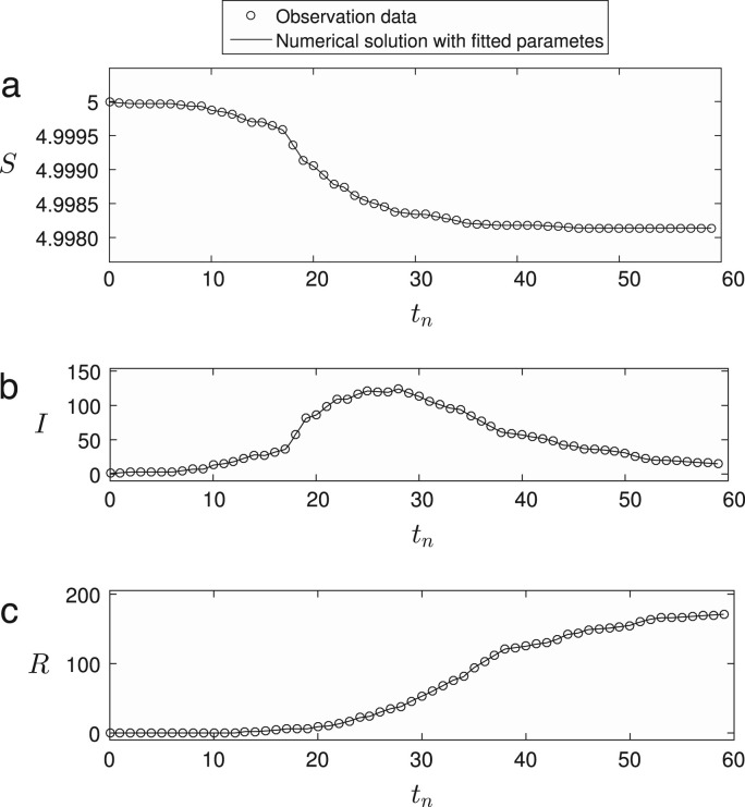
In all computations, the initial conditions are taken to be $N=500\text{,}000$, $S^0=N-1$, $I^0=1$, and $R^0=0$ with $t_{\mathrm{ref}}=20$ May 2015. Fig. 2 shows the time series of observed MERS-CoV epidemiological data and numerical solutions $S$, $I$, and $R$, respectively.

Fig. 2.

Time series of observed MERS-CoV epidemiological data and numerical solutions of (a) $S$, (b) $I$, and (c) $R$, respectively. Here, $N=500\text{,}000$ is used.

The basic reproduction number $R_0$ is the average number of secondary infections caused by one infectious individual in a completely susceptible population. It is an important measurement in that one can determine the stability of the disease-free equilibrium by computing the value of $R_0$; $R_0<1$ implies that the disease-free equilibrium is locally asymptotically stable  [17], and if $R_0>1$, it is unstable  [18], [19]. Finding basic reduction number $R_0$ can be done through the next generation matrix  [20], [21] whose spectral radius is defined as $R_0$. In the SIR model, the basic reproduction number is computed as $R_0=\beta N/\gamma$   [22], [23], which will be used for our method in the next section.

4.1. Weighted averaging basic reproduction number $R_{0,k,\omega }^n$

In this section, we propose the weighted average values for infected and removed rates, and then define weighted averaging basic reproduction number. Let ${\beta }_{1,1}^n={\beta }^n$ for $n=1,\dots ,m$. We define $k$-days ($k\ge 2$) weighted average ${\beta }_{k,\omega }^n$ as

$${\beta }_{k,\omega }^n=\{\begin{array}{c}\sum _{i=1}^k\left({\omega }^{i-1}{\beta }^{n-i+1}\right)/\sum _{i=1}^k{\omega }^{i-1}\text{if }n\ge k\text{,}\\ \sum _{i=1}^n\left({\omega }^{i-1}{\beta }^{n-i+1}\right)/\sum _{i=1}^n{\omega }^{i-1}\text{if }n<k\text{,}\end{array}$$ (11)

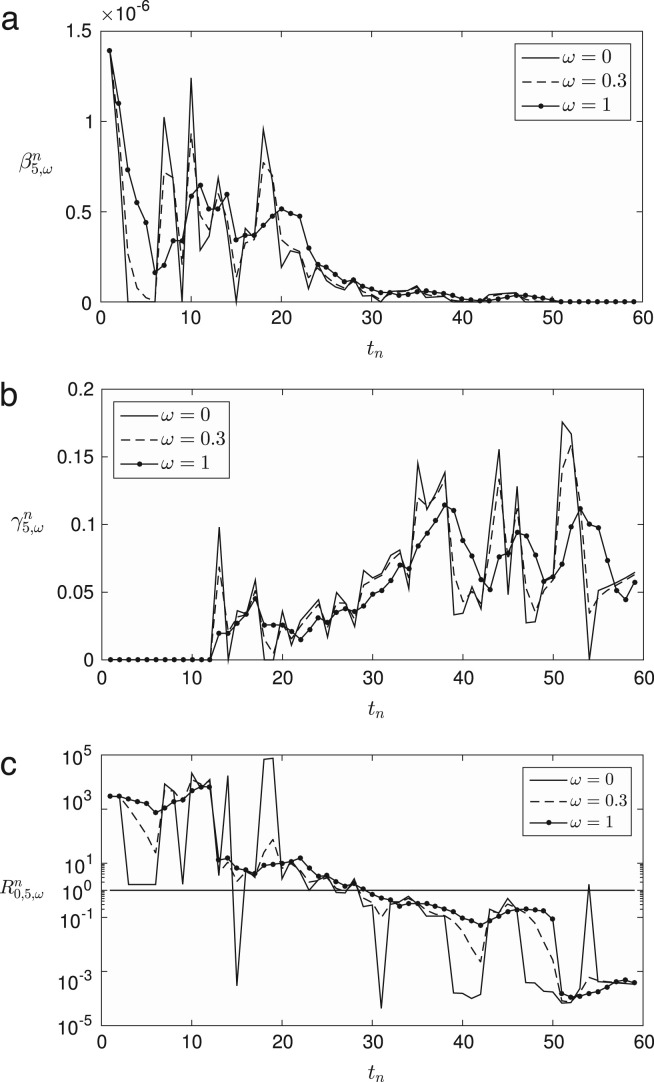
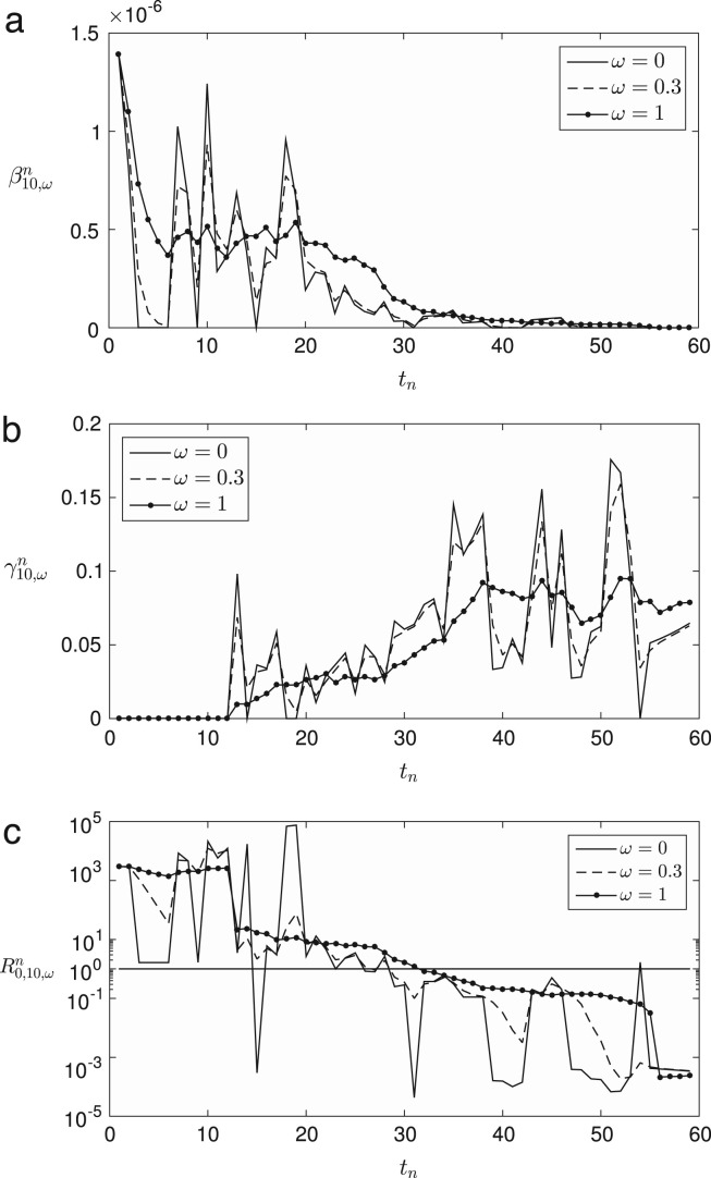
where $0<\omega \le 1$ and the superscript $i-1$ for ${\omega }^{i-1}$ represents an exponent. Also, ${\gamma }_{k,\omega }^n$ is defined similarly as Eq. (11). Finally, we define the daily computed weighted averaging basic reproduction number as $R_{0,k,\omega }^n={\beta }_{k,\omega }^{n}N/{\gamma }_{k,\omega }^n$. Fig. 3 (a)–(c) represent ${\beta }_{k,\omega }^n$, ${\gamma }_{k,\omega }^n$, and $R_{0,k,\omega }^n$ for $k=5$, respectively, with $w=0$, 0.3, and 1. Fig. 4 shows the results of the parameters for $k=10$. Note that when $\omega =0$, we have $R_{0,k,0}^n=R_{0,1,0}^n$ for all $k$. If $k$ is large, then we have more smooth profile and the transition point ($R_{0,k,\omega }^n=1$) moves to the right. If $\omega$ is close to zero, then we have a similar profile to $R_{0,1,0}^n$. Note that we have extraordinarily large values of $R_{0,k,\omega }^n$ from $n=1$ to approximately $n=20$ since the recovered individuals were almost zero (${\gamma }_{k,\omega }^n\approx 0$) in early times and the infected ones increased rapidly.

Fig. 3.

Weighted averaging ${\beta }_{k,\omega }^n$, ${\gamma }_{k,\omega }^n$, and $R_{0,k,\omega }^n$ for $k=5$. In each case, we compare the values with $\omega =0$, 0.3, and 1.

Fig. 4.

Weighted averaging ${\beta }_{k,\omega }^n$, ${\gamma }_{k,\omega }^n$, and $R_{0,k,\omega }^n$ for $k=10$. In each case, we compare the values with $\omega =0$, 0.3, and 1.

4.2. Predictability of a linear extrapolation, $R_{\mathrm{linear}}^n$

In this section, we investigate the predictability of a linear extrapolation of $R_{0,1,0}^n$. Let us define the linear extrapolation

$$R_{\mathrm{linear}}^n=2R_{0,1,0}^{n-1}-R_{0,1,0}^{n-2}\text{,}\text{for }3\le n\le m\text{,}$$ (12)

where $R_{\mathrm{linear}}^n$ means the predicted reproduction number based on the previous two consecutive reproduction numbers and the error is defined as

$$E^n=R_{\mathrm{linear}}^n-R_{0,1,0}^n\text{,}\text{for }3\le n\le m\text{.}$$ (13)

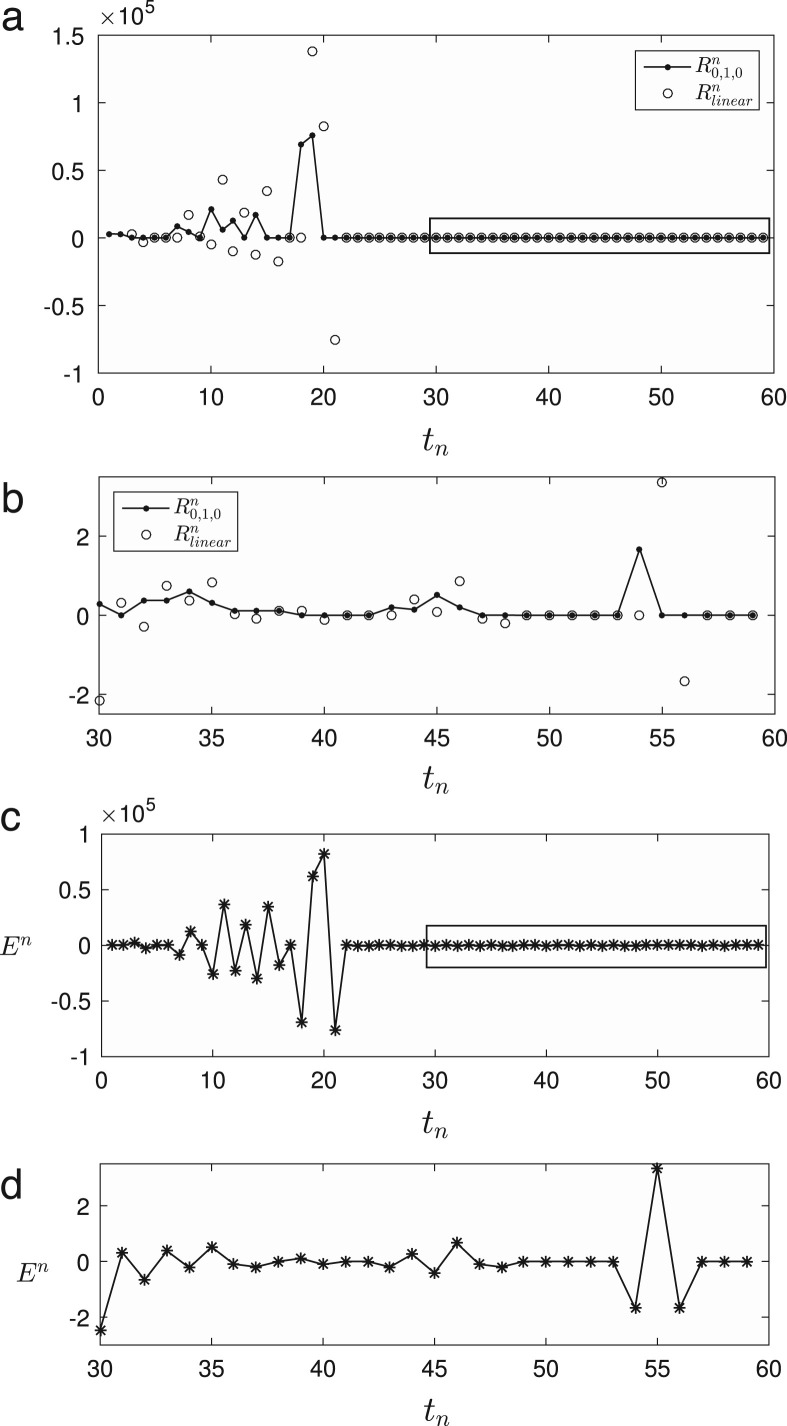
Fig. 5(a) shows $R_{\mathrm{linear}}^n$ and $R_{0,1,0}^n$. Up to about three weeks, there are large differences between two reproduction numbers. However, we can observe a good agreement interval from $n=30$ to $n=59$, see Fig. 5(b). Fig. 5(c) and (d) are corresponding errors $E^n$ of (a) and (b). The errors $E^n$ from $n=30$ to $n=59$ are listed in Table 1 . Except some days, the absolute errors $\left|E^n\right|$ are less than one. We note that we have a spike in Fig. 5(b) and (d). That is due to no population data changes for two days, i.e., 11 July and 12 July as shown in Fig. 1.

Fig. 5.

(a) Comparison of the $R_{0,1,0}^n$ with $R_{\mathrm{linear}}^n$ which are denoted by the symbols ($\cdot$) and ($\circ$), respectively. (b) A magnified view of a rectangular box in (a). (c) Error for $R_{0,1,0}^n$ from 20 May 2015 to 17 July 2015. (d) A magnified view of a rectangular box in (c) from 18 June 2015 to 17 July 2015.

Table 1.

Error which is expressed by $E^n=R_{\mathrm{linear}}^n-R_{0,1,0}^n$ from 18 June, 2015 to 17 July, 2015, i.e., $n=30,\dots ,59$.

$n$	$E^n$	$n$	$E^n$	$n$	$E^n$
30	−2.4532	40	−0.1110	50	−0.0002
31	+0.3215	41	+0.0000	51	+0.0001
32	−0.6608	42	−0.0001	52	−0.0001
33	+0.3751	43	−0.1999	53	−0.0002
34	−0.2251	44	+0.2571	54	−1.6766
35	+0.5175	45	−0.4144	55	+3.3534
36	−0.0958	46	+0.6574	56	−1.6766
37	−0.1967	47	−0.1004	57	−0.0000
38	−0.0000	48	−0.1997	58	+0.0009
39	+0.1110	49	+0.0002	59	−0.0000

4.3. The SIR model with disease-related death

In this section, we consider the modified SIR model with disease-related death. Let the total population $N$ be divided into susceptible $S\left(t\right)$, infected $I\left(t\right)$, recovered $R\left(t\right)$, and dead $D\left(t\right)$ individuals at time $t$, then the SIR model with fatality rate is given by

$$\frac{dS\left(t\right)}{dt}=-\beta \left(t\right)S\left(t\right)I\left(t\right)\text{,}$$ (14)

$$\frac{dI\left(t\right)}{dt}=\beta \left(t\right)S\left(t\right)I\left(t\right)-\gamma \left(t\right)I\left(t\right)-d\left(t\right)I\left(t\right)\text{,}$$ (15)

$$\frac{dR\left(t\right)}{dt}=\gamma \left(t\right)I\left(t\right)\text{,}$$ (16)

$$\frac{dD\left(t\right)}{dt}=d\left(t\right)I\left(t\right)$$ (17)

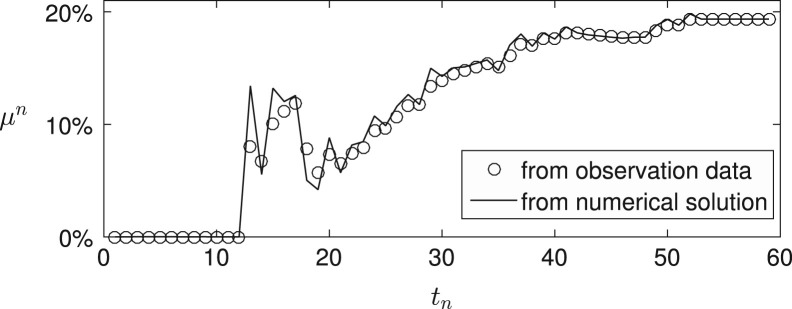
with initial condition $S\left(0\right)=S^0$, $I\left(0\right)=I^0$, $R\left(0\right)=R^0$, and $D\left(0\right)=D^0$. Here, the time-dependent parameters $\beta \left(t\right)$, $\gamma \left(t\right)$, and $d\left(t\right)$ denote the contact, recovered, and dead rates from disease, respectively  [22]. Now, by using the proposed method, we evaluate the numerical solution of the modified SIR model (14), (15), (16), (17). We take the same initial conditions: $N=500\text{,}000$, $S^0=N-1$, $I^0=1$, $R^0=0$, and $D^0=0$. The initial guesses for finding coefficients $\beta$, $\gamma$, and $d$ are 1.0e−6, 1.0e−1, and 1.0e−1, respectively. Using this model, we can predict the ratio of individuals who died by disease to the infected population at a given time. To investigate the ratio, we introduce the fatality percentage rate ${\mu }^n$ which is defined as

$${\mu }^n=\frac{D^n}{I^n+R^n+D^n}\times 100\left(\%\right)\text{.}$$

In Fig. 6 , we show the fatality percentage rate ${\mu }^n$ from the real observation data and the numerical approximations. Here, the fatality percentage rate ${\mu }^n$ from the numerical approximation is obtained by the numerical solutions $S^n$, $I^n$, $R^n$, and $D^n$. The numerical solutions $S^n$, $I^n$, $R^n$, and $D^n$ are evaluated by using the best-fitting parameters ${\beta }^{n-1}$, ${\gamma }^{n-1}$, and $d^{n-1}$ at time $t_{n-1}$. As shown in Fig. 6, the both results are in good agreement in later times.

Fig. 6.

Fatality percentage rate ${\mu }^n$ by the observation data (circle marker) and the numerical approximations (solid line).

5. Conclusion

We have proposed the daily computed weighted averaging basic reproduction number $R_{0,k,\omega }^n$ for MERS-CoV outbreak in South Korea, May to July 2015. The linearly extrapolated reproduction number, $R_{\mathrm{linear}}^n$, has important implications for the future prediction of the trend of the reproduction numbers. We showed that the results computed by our method match very well with the actual data of the MERS-CoV spread in South Korea. Using the method proposed in this paper, one can predict the progress of the spread of infections on the use of real-time epidemic data, so that proper control policies can be performed in an appropriate time for reducing the spread of the infections. As future research, the methodology introduced in this paper can be applied to various diseases with other epidemic spreading models.

Appendix.

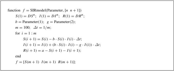
In this section, we present the parameter fitting algorithm using the MATLAB function lsqcurvefit, which finds the optimal parameters in the least-squares sense. The following command returns the optimal parameters.

In this routine, ${\beta }^0$ and ${\gamma }^0$ are an initial guess, $[nn+1]$ is a time interval, and $\text{SIRdata}=\left[D{S}^{n+1}D{I}^{n+1}D{R}^{n+1}\right]$. Also, $\left[00\right]$ and $\left[11\right]$ represent the lower and upper bounds for the fitting parameters ${\beta }^{n+1}$ and ${\gamma }^{n+1}$. Here, the function SIRmodel is given as follows.

References

- 1.Zhang X., Ge B., Wang Q., Jiang J., You H., Chen Y. Epidemic spreading characteristics and immunity measures based on complex network with contact strength and community structure. Math. Probl. Eng. 2015;2015:12. Article ID 316092. [Google Scholar]
- 2.Cowling B.J., Park M., Fang V.J., Wu P., Leung G.M., Wu J.T. Preliminary epidemiologic assessment of MERS-CoV outbreak in South Korea, May–June 2015. Euro Surveill. 2015;20 doi: 10.2807/1560-7917.es2015.20.25.21163. [DOI] [PMC free article] [PubMed] [Google Scholar]
- 3.Korea Ministry of Health and Welfare (KMOHW) and Korean Centers for Disease Control and Prevention (KCDC). MERS portal (Daily report), http://www.mers.go.kr.
- 4.Korea Ministry of Health and Welfare (KMOHW) and Korean Centers for Disease Control and Prevention (KCDC). Daily report for number of infected, recovered, and dead people. http://www.mw.go.kr/, http://cdc.go.kr/CDC/.
- 5.Kermack W.O., McKendrick A.G. A contribution to the mathematical theory of epidemics. Proc. R. Soc. Lond. Ser. A: Math. Phys. Eng. Sci. 1927;115:700–721. [Google Scholar]
- 6.Ji C., Jiang D., Shi N. Multigroup SIR epidemic model with stochastic perturbation. Physica A. 2011;390:1747–1762. [Google Scholar]
- 7.Tanaka M., Sakumoto Y., Aida M., Kawashima K. 2015 10th Asia-Pacific Symposium on Inform. Telecommun. Technol. (APSITT) IEEE; 2015. Study on the growth and decline of SNSs by using the infectious recovery SIR model. [Google Scholar]
- 8.Gomes M.F.C., Goncalves S. SIR model with general distribution function in the infectious period. Physica A. 2009;388:3133–3142. [Google Scholar]
- 9.Tornatore E., Buccellato S.M., Vetro P. Stability of a stochastic SIR system. Physica A. 2005;354:111–126. [Google Scholar]
- 10.Ji C., Jiang D., Shi N. The behavior of an SIR epidemic model with stochastic perturbation. Stoch. Anal. Appl. 2012;30:755–773. [Google Scholar]
- 11.Shulgin B., Stone L., Agur Z. Pulse vaccination strategy in the SIR epidemic model. Bull. Math. Biol. 1998;60:1123–1148. doi: 10.1006/S0092-8240(98)90005-2. [DOI] [PubMed] [Google Scholar]
- 12.Stone L., Shulgin B., Agur Z. Theoretical examination of the pulse vaccination policy in the SIR epidemic model. Math. Comput. Modelling. 2000;31:207–215. [Google Scholar]
- 13.Fu L., Song W., Lv W., Lo S. Simulation of emotional contagion using modified SIR model: A cellular automaton approach. Physica A. 2014;405:380–391. [Google Scholar]
- 14.Mandal S., Sarkar R.P., Sinha S. Mathematical models of malaria-a review. Malar. J. 2011;10:1–19. doi: 10.1186/1475-2875-10-202. [DOI] [PMC free article] [PubMed] [Google Scholar]
- 15.S. Polwiang, The seasonal reproduction number of dengue fever impacts of climate on transmission, PeerJ PrePrints e1142 2015. 10.7287/peerj.preprints.756v2. [DOI] [PMC free article] [PubMed] [Retracted]
- 16.Duncan C.J., Duncan S.R., Scott S. Whooping cough epidemics in London, 1701-1812: infection dynamics, seasonal forcing and the effects of malnutrition. Proc. R. Soc. Lond. B: Biol. Sci. 1996;263:445–450. doi: 10.1098/rspb.1996.0067. [DOI] [PubMed] [Google Scholar]
- 17.Wang Y., Cao J., Alofi A., Abdullah A.M., Elaiw A. Revisiting node-based SIR models in complex networks with degree correlations. Physica A. 2015;437:75–88. [Google Scholar]
- 18.Driessche V.D., Watmough J. Reproduction numbers and sub-threshold endemic equilibria for compartmental models of disease transmission. Math. Biosci. 2002;180:29–48. doi: 10.1016/s0025-5564(02)00108-6. [DOI] [PubMed] [Google Scholar]
- 19.Chowell G., Abdirizak F., Lee S., Lee J., Jung E., Nishiura H., Viboud C. Transmission characteristics of MERS and SARS in the healthcare setting: a comparative study. BMC Med. 2015;13:210–221. doi: 10.1186/s12916-015-0450-0. [DOI] [PMC free article] [PubMed] [Google Scholar]
- 20.Diekmann O., Heesterbeek H. Wiley; New York: 2002. Mathematical Epidemiology of Infectious Diseases: Model Building, Analysis and Interpretation. [Google Scholar]
- 21.Heesterbeek J.A.P. A brief history of and a recipe for its calculation. Acta Biotheor. 2002;50:189–204. doi: 10.1023/a:1016599411804. [DOI] [PubMed] [Google Scholar]
- 22.Britton N. Springer Science & Business Media; 2012. Essential Mathematical Biology. [Google Scholar]
- 23.Chowell G., Blumberg S., Simonsen L., Miller M.A., Viboud C. Synthesizing data and models for the spread of MERS-CoV, 2013: Key role of index cases and hospital transmission. Epidemics. 2014;9:40–51. doi: 10.1016/j.epidem.2014.09.011. [DOI] [PMC free article] [PubMed] [Google Scholar]