Optimal control for SIRC epidemic outbreak

Abstract

In this paper the mathematical SIRC epidemic model is considered. It efficiently describes diseases in which a cross immune class (C) is present, along with the susceptible (S), the infected (I) and the removed (R) ones. Controlling epidemic diseases corresponds to the introduction of vaccination, quarantine and treatment strategies; generally only one of these actions is considered. In this paper the possibility of optimal controls both over the susceptible and the infected subjects is assumed, taking into account also limitations of resources. A suitable cost index is introduced and via the Pontryagin's Minimum Principle the optimal control strategy is determined and the existence of the optimal solution is assessed. Numerical results are developed analyzing the effects of different control strategies.

1. Introduction

Mathematical models have become important instruments in the analysis and control of infectious diseases. Several models corresponding to epidemic with different characteristics have been proposed and discussed in literature. The fundamental assumption in epidemic models is that the population can be divided into distinct groups; the most common are: the susceptible (S) that are the subjects that may catch the disease; the infected (I) that are the subjects that are already infected and can spread the disease to susceptible individuals; the removed (R) that are the subject that are immune for life. Therefore these models are referred to as SIR models. Other descriptions may include the presence of subjects in the quarantine state (Q) and in this situation SIRQ models are analyzed [1]. Recently in [2] the class of cross-immune individuals (C) in the population has been introduced: it is an intermediate state between the fully susceptible state (S) and the fully protected one (R). Therefore the obtained SIRC model takes into account temporary partial immunity and may well describe, for example, influenza A.

The study of mathematical models for epidemics allows the evaluation of the effects of different control strategies: the scheduling of a proper vaccination campaign [3], [4], the screening and educational campaigns [5], isolation policy [6], the resource allocation [5], [7]. An encouraging approach lies in the framework of the optimal control theory; interesting reviews can be found in [8]. Analytical results on the optimal control problems for epidemics were extensively described in [9], where models with control by vaccination, quarantine, screening or health campaigns were studied with a rather general choice for the interaction function.

Different kind of infectious disease calls for different models and strategies. In [10] the severe acute respiratory syndrome (SARS) disease was considered to find the strategy of tracing and quarantining contacts of identified cases; it was shown that this can be very successful in reducing transmission. In [11] it was proved that a maximum quarantine/isolation measures for the exposed and the infectious class would reduce the SARS epidemics; a bang–bang switching control was obtained. In the last decade great attention has been devoted to the modeling and control of the human immunodeficiency virus (HIV) infection; in [12] an output feedback scheme based in CD4 T-cell and viral load measurements has been introduced. For the control in Dengue epidemics optimal and sub-optimal strategies were considered in [13]; the effects of educational campaigns organized to motivate the population to break the reproduction cycle of the mosquitoes by avoiding the accumulation of still water in open-air recipients were modeled and the assumed cost index reflected a compromise between actual financial spending and population health. Optimal and suboptimal solutions were introduced also in [14] with reference to quarantine and isolation control in SARS epidemics, demonstrating that the maximal applications of the control strategies in the early stage of the epidemic were of very significant impact in both the considered control cases.

In this paper the SIRC model is considered aiming at the control of the epidemic spreading, taking into account the limitations of the resources. Among the cause of death related with influenza, pneumonia, heart and circulatory are the most significant; moreover most of these deaths are in individuals in the age group over 65 years whereas younger children are at significant risk of influenza hospitalization. These considerations lead to recommendation of vaccination for subjects above 64 years (59 in some countries) and for young children (above 6 months). Characteristic of influenza is its seasonality; the peaks of the influenza are related with the weather condition, and social patterns, for example schools holidays.

In this paper, in the framework of multiple optimal controls [15], [16], [17], the controls both in the susceptible and in the infected class are introduced and the existence of the optimal solution is assessed in the SIRC epidemic model. Note that a similar approach was presented in [18] with reference to vector-borne diseases and not considering the cross-immune class.

The paper is organized as follows; in Section 2 the SIRC model is described and an optimal control strategy is introduced; the proposed control action is analyzed and existence results are assessed. In Section 3 numerical results are presented and discussed.

2. Materials and methods

2.1. The SIRC model and the introduction of control strategy

The SIRC model introduced by [2] considered the presence of susceptible, infectious, removed and cross immune subjects:

$$\begin{array}{l}\dot{S}(t)=\mu (1-S(t))-\beta S(t)I(t)+\gamma C(t)\hfill \\ \dot{I}(t)=\beta S(t)I(t)+\sigma \beta C(t)I(t)-(\mu +\alpha )I(t)\hfill \\ \dot{R}(t)=(1-\sigma )\beta C(t)I(t)+\alpha I(t)-(\mu +\delta )R(t)\hfill \\ \dot{C}(t)=\delta R(t)-\beta C(t)I(t)-(\mu +\gamma )C(t)\hfill \end{array}$$ (1)

with initial conditions:

$$S(0)=S_0,I(0)=I_0,R(0)=R_0,C(0)=C_0$$ (2)

and positive real parameters: α, β, δ, γ, μ, σ. In Fig. 1 the scheme of the SIRC model is represented. The parameters α, δ and γ are the inverses of the average time spent by the subjects in the compartments I, R and C respectively. The parameter μ represents the mortality rate in every compartment and, following the suggestion in [2], is assumed equal to the rate of newborn in the population; the parameter σ may be interpreted as the average reinfection probability of a cross-immune subject, whereas the parameter β is the contact rate. There are some relations among the model parameters: $\beta =\overline{R}(\mu +\alpha )$ and σ  =  r(1/δ  + 1/γ), with $2\le \overline{R}\le 10$ and r  ≈ 0.026 (year)⁻¹; in particular, $\overline{R}$ represents the reproduction number [19] whereas r represents the rate of infection [20].

Fig. 1.

Block diagram of the adopted SIRC model.

The novelty of this model is that it takes into account the presence of cross-immune (C) subjects, i.e. subjects that are temporarily immune. It efficiently describes the mechanism for influenza A viruses.

In this paper the effects of control strategies over both susceptible subjects (i.e. vaccination) and infected ones (treatment and quarantine) are studied. To this aim additive terms must be suitable introduced in the differential equation relative to susceptible, to immune and to removed subjects:

$$\begin{array}{l}\dot{S}(t)=\mu (1-S(t))-\beta S(t)I(t)+\gamma C(t)-g(S(t),u(t))\hfill \\ \dot{I}(t)=\beta S(t)I(t)+\sigma \beta C(t)I(t)-(\mu +\alpha )I(t)-h(I(t),v(t))\hfill \\ \dot{R}(t)=(1-\sigma )\beta C(t)I(t)+\alpha I(t)-(\mu +\delta )R(t)+g(S(t),u(t))+h(I(t),v(t))\hfill \\ \dot{C}(t)=\delta R(t)-\beta C(t)I(t)-(\mu +\gamma )C(t)\hfill \end{array}$$ (3)

with initial conditions equal to (2) and with the bounds:

$$u_{\min }\le u(t)\le u_{\max }{v}_{\min }\le v(t)\le v_{\max }$$ (4)

The functions g(S(·), u(·)) and $h(I(\cdot ),v(\cdot ))$ represent the actions of the control effort; the former models the control over the susceptible, for example a vaccination action, whereas the latter represents the treatment and/or quarantine action. Different mathematical descriptions for these strategies could be adopted; the expression proposed in [21] has been assumed (note that in the cited paper only the control by vaccination was introduced):

$$g(S(t),u(t))={\rho }_{1}S(t)u(t)$$ (5)

$$h(I(t),v(t))={\rho }_{2}I(t)v(t)$$ (6)

with ρ ₁,ρ ₂  > 0.

2.2. Existence of the solution of the control system

To discuss the existence of the solution of control system (3) with the above conditions (5), (6), the classical arguments applied in [21] may be followed; the system (3) may be rewritten:

$$\frac{dx(t)}{dt}=Ax+F(x)$$ (7)

where $x(t)={(\begin{array}{cccc}\hfill S(t)\hfill & \hfill I(t)\hfill & \hfill R(t)\hfill & \hfill C(t)\hfill \end{array})}^T$ is the vector of the state variables, A and F(x) are defined as follows:

$$A=\left(\begin{array}{cccc}\hfill -\mu -{\rho }_{1}u\hfill & \hfill 0\hfill & \hfill 0\hfill & \hfill \gamma \hfill \\ \hfill 0\hfill & \hfill -(\mu +\alpha )-{\rho }_{2}v\hfill & \hfill 0\hfill & \hfill 0\hfill \\ \hfill {\rho }_{1}u\hfill & \hfill {\rho }_{2}v+\alpha \hfill & \hfill -(\mu +\delta )\hfill & \hfill 0\hfill \\ \hfill 0\hfill & \hfill 0\hfill & \hfill \delta \hfill & \hfill -(\mu +\gamma )\hfill \end{array}\right)$$ (8)

$$F(x)=\left(\begin{array}{c}\hfill -\beta S(t)I(t)+\mu \hfill \\ \hfill \beta S(t)I(t)+\sigma \beta C(t)I(t)\hfill \\ \hfill (1-\sigma )\beta C(t)I(t)\hfill \\ \hfill \beta C(t)I(t)\hfill \end{array}\right)$$ (9)

From the Holder inequality, the second term of the right end side of Eq. (7) satisfies:

$$|F(x_1)-F(x_2)|\le M(|S_1-S_2|+|I_1-I_2|+|C_1-C_2|)$$ (10)

where the positive constant M is independent of the state variables x.

Let set G(x) =  Ax  +  F(x); we get:

$$|G(x_1)-G(x_2)|\le Q|x_1-x_2|$$ (11)

where $Q=\max \left\{M,∥A∥\right\}<\infty$. Therefore the function G is uniformly Lipschitz continuous. The solution of the system (7) exists from (11) and taking into account the constraints on the controls u and v and the restrictions on the non-negativeness of the state variables [22].

2.3. Optimal control strategy

Let us define the following cost index:

$$J(x,u,v)={\int }_{t_i}^{t_f}L(x,u,v)={\int }_{t_i}^{t_f}\left[{\alpha }_{1}S(t)+{\alpha }_{2}I(t)+\frac{1}{2}{\tau }_1{u}^2(t)+\frac{1}{2}{\tau }_2{v}^2(t)\right]dt$$ (12)

with α ₁,α ₂, τ ₁,τ ₂  > 0 representing the weights in the cost index, t _i  ≥ 0 is the fixed initial time and t _f  > 0 is the fixed final time of the control interval. The aim is to minimize the infected and susceptible individuals and to maximize the total number of removed subjects using minimal control efforts. Obviously the adopted cost index takes into account also the more common case in which the objective is to minimize only the infected subjects, and not also the susceptible ones.

Let us consider the following problem.

Problem: Given the model (3) with initial conditions (2), determine the state x° and the controls u and v satisfying the system (3), the conditions (4) and that minimize the cost index (12).

The aim is to determine the best strategy that minimizes the number of susceptible and infected subjects and the control resources in the fixed control interval.

Let's now previously discuss the existence of the optimal control. It is guaranteed by the following arguments [23]:

• 1.The set of controls and state variables is non-empty
• 2.The control space is closed and convex
• 3.The right hand side of the state system is bounded by a linear function in the state and control
• 4.The integrand in the cost index is convex with respect to the controls u and v
• 5.
  There exists a constant η  > 1 and positive numbers β ₁ and β ₂ such that:

  $$J(u(t),v(t))\ge {\beta }_2{(|u(t){|}^2+|v(t){|}^2)}^{\eta /2}-{\beta }_1$$ (13)

Condition 1 is satisfied by the result in [24], theorem 9.2.1; condition 2 is verified by definition. Condition 3 follows from the arguments in the previous Subsection. The integrand is obviously convex with respect to the controls u and v. Condition 5 and disequation (13) follow taking into account that the state variables are bounded.

Now we will solve the optimal control problem and we denote by U  = (u   v) the collection of the admissible controls that are the two controls satisfying the constraints (4). Let us define the Hamiltonian:

$$H(x(t),U(t),{\lambda }_0,\lambda (t))={\lambda }_{0}L(x(t),u(t),v(t))+{\lambda }^T(t)f(x(t),u(t),v(t))={\lambda }_0\left[{\alpha }_{1}S(t)+{\alpha }_{2}I(t)+\frac{1}{2}{\tau }_1{u}^2(t)+\frac{1}{2}{\tau }_2{v}^2(t)\right]+{\lambda }_1(t)[\mu (1-S(t))-\beta S(t)I(t)+\gamma C(t)-{\rho }_{1}u(t)S(t)]+{\lambda }_2(t)[\beta S(t)I(t)+\sigma \beta C(t)I(t)-(\mu +\alpha )I(t)-{\rho }_{2}v(t)I(t)]+{\lambda }_3(t)[(1-\sigma )\beta C(t)I(t)+\alpha I(t)-(\mu +\delta )R(t)+{\rho }_{1}u(t)S(t)+{\rho }_{2}v(t)I(t)]+{\lambda }_4(t)[\delta R(t)-\beta C(t)I(t)-(\mu +\gamma )C(t)]$$ (14)

where λ ₀ and λ are the Lagrange multipliers. From the minimum principle of Pontryagin (for a survey of different formulations of the minimum principle see, for example [25]), the following result holds.

Let (x*U*) satisfies the dynamic control system (3), the initial condition (2) and the constraint (4). It is an optimal solution (global minimum) if there exist a constant λ ₀  ≥ 0, functions ${\lambda }^{*}\in {\overline{C}}^1[t_i,t_f]$ not simultaneous equal to zero such that:

$$\begin{array}{l}{\dot{\lambda }}^{*}=-{\left(\frac{\partial H}{\partial x}\right|}^{*T}\hfill \\ H(x^{*}(t),\omega ,{{\lambda }_0}^{*},{\lambda }^{*}(t))\ge H(x^{*}(t),U^{*}(t),{{\lambda }_0}^{*},{\lambda }^{*}(t))\forall \text{admissible control}\omega \hfill \\ {\left(H\right|}^{*}=0\hfill \\ \lambda (t_f)=0\hfill \end{array}$$ (15)

The notation ${\overline{C}}^1[t_i,t_f]$ denotes all the function piece-wise continuously differentiable. Note that the singular case λ ₀  = 0 is not possible; in fact in this case, taking into account the last condition in (15), the existence and uniqueness theorem for differential equations implies λ ₁  =  λ ₂  =  λ ₃  =  λ ₄  = 0 which is impossible.

Let's particularize the necessary condition of optimality assuming λ ₀  = 1:

$$\begin{array}{l}{\dot{\lambda }}_1^{*}(t)=-{\left(\frac{\partial H(x(t),U(t),\lambda (t))}{\partial S}\right|}^{*T}=-[{\alpha }_1+{\lambda }_1^{*}(t)(-\mu -\beta I(t)-{\rho }_1{u}^{*}(t))+{\lambda }_2^{*}(t)\beta I(t)+{\lambda }_3^{*}(t)({\rho }_1{u}^{*}(t))]\hfill \\ {\dot{\lambda }}_2^{*}(t)=-{\left(\frac{\partial H(x(t),U(t),\lambda (t))}{\partial I}\right|}^{*T}=-[{\alpha }_2-{\lambda }_1^{*}(t)\beta S(t)+{\lambda }_2^{*}(\beta S(t)+\sigma \beta C(t)-(\mu +\alpha )-{\rho }_2{v}^{*}(t))+{\lambda }_3^{*}(t)((1-\sigma )\beta C(t)+\alpha +{\rho }_2{v}^{*}(t))-{\lambda }_4^{*}(t)\beta C(t)]\hfill \\ {\dot{\lambda }}_3^{*}(t)=-{\left(\frac{\partial H(x(t),U(t),\lambda (t))}{\partial R}\right|}^{*T}={\lambda }_3^{*}(t)(\mu +\delta )-{\lambda }_4^{*}(t)\delta \hfill \\ {\dot{\lambda }}_4^{*}(t)=-{\left(\frac{\partial H(x(t),U(t),\lambda (t))}{\partial C}\right|}^{*T}=-{\lambda }_1^{*}(t)\gamma -{\lambda }_2^{*}\sigma \beta I(t)-{\lambda }_3^{*}(t)(1-\sigma )\beta I(t)-{\lambda }_4^{*}(t)(-\beta I(t)-(\mu +\gamma ))\hfill \end{array}$$ (16)

$$\frac{1}{2}{\tau }_{1}u{*}^2(t)+\frac{1}{2}{\tau }_{2}v{*}^2(t)-{\lambda }_1^{*}(t){\rho }_1{u}^{*}(t)S(t)-{\lambda }_2^{*}(t){\rho }_2{v}^{*}(t)I(t)+{\lambda }_3^{*}(t)[{\rho }_1{u}^{*}(t)S(t)+{\rho }_2{v}^{*}(t)I(t)]\le \frac{1}{2}{\tau }_1{\overline{u}}^2(t)+\frac{1}{2}{\tau }_2{\overline{v}}^2(t)-{\lambda }_1^{*}(t){\rho }_1\overline{u}(t)S(t)-{\lambda }_2^{*}(t){\rho }_2\overline{v}(t)I(t)+{\lambda }_3^{*}(t)[{\rho }_1\overline{u}(t)S(t)+{\rho }_2\overline{v}(t)I(t)]\forall (\overline{u}(t),\overline{v}(t))\text{admissible control}$$ (17)

$${\left(H\right|}^{*}=0$$ (18)

$${\lambda }_1(t_f)={\lambda }_2(t_f)={\lambda }_3(t_f)={\lambda }_4(t_f)=0$$ (19)

Exploiting the minimum condition (17) it follows:

$$\begin{array}{l}{\left(\frac{\partial H}{\partial u}\right|}^{*}={\tau }_1{u}^{*}(t)-{\lambda }_1^{*}(t){\rho }_{1}S(t)+{\lambda }_3^{*}(t){\rho }_{1}S(t)=0\Rightarrow u^{*}(t)=\frac{{\rho }_{1}S(t)}{{\tau }_1}({\lambda }_1^{*}(t)-{\lambda }_3^{*}(t))\hfill \\ {\left(\frac{\partial H}{\partial v}\right|}^{*}={\tau }_2{v}^{*}(t)-{\lambda }_2^{*}(t){\rho }_{2}I(t)+{\lambda }_3^{*}(t){\rho }_{2}I(t)=0\Rightarrow v^{*}(t)=\frac{{\rho }_{2}I(t)}{{\tau }_2}({\lambda }_2^{*}(t)-{\lambda }_3^{*}(t))\hfill \end{array}$$ (20)

And therefore, taking into account the box constraints on the controls, we obtain:

$$u^{*}(t)=\left\{\begin{array}{ll}0\hfill & \text{if}\frac{{\rho }_{1}S(t)}{{\tau }_1}({\lambda }_1^{*}(t)-{\lambda }_3^{*}(t))\le 0\hfill \\ \frac{{\rho }_{1}S(t)}{{\tau }_1}({\lambda }_1^{*}(t)-{\lambda }_3^{*}(t))\hfill & \text{if}0<\frac{{\rho }_{1}S(t)}{{\tau }_1}({\lambda }_1^{*}(t)-{\lambda }_3^{*}(t))<0.9\hfill \\ 0.9\hfill & \text{if}\frac{{\rho }_{1}S(t)}{{\tau }_1}({\lambda }_1^{*}(t)-{\lambda }_3^{*}(t))\ge 0.9\hfill \end{array}\right)$$ (21)

and

$$v^{*}(t)=\left\{\begin{array}{ll}0\hfill & \text{if}\frac{{\rho }_{2}I(t)}{{\tau }_2}({\lambda }_2^{*}(t)-{\lambda }_3^{*}(t))\le 0\hfill \\ \frac{{\rho }_{2}I(t)}{{\tau }_2}({\lambda }_2^{*}(t)-{\lambda }_3^{*}(t))\hfill & \text{if}0<\frac{{\rho }_{2}I(t)}{{\tau }_2}({\lambda }_2^{*}(t)-{\lambda }_3^{*}(t))<0.9\hfill \\ 0.9\hfill & \text{if}\frac{{\rho }_{2}I(t)}{{\tau }_2}({\lambda }_2^{*}(t)-{\lambda }_3^{*}(t))\ge 0.9\hfill \end{array}\right)$$ (22)

In the next section we discuss the numerical solution of the optimal control problem.

3. Results and discussion

In this section the necessary conditions (16), (17), (18), (19) are studied, from a numerical point of view; they are solved by using the © Matlab Optimization Toolbox and the function fmincon. It allows the finding of a constrained minimum of a function of several variables; this function uses sequential quadratic programming method [26]. It solves a quadratic programming subproblem [27] at each iteration in which a positive definite quasi-Newton approximation of the Hessian of the Lagrangian function was updated using the Broyden–Fletcher–Goldfarb–Shanno method [28]. Eq. (3) were discretized by using the classical trapezoidal rule dividing the time duration interval into n  − 1 equally spaced subintervals; in the simulation we assumed n  = 500 with ad hoc integration step in order to simulate a control period of one year.

To discuss the effects of the control strategy over the number of susceptible and infectious subjects, the following values for the SIRC model were adopted:$\mu =\frac{1}{75}{(\text{year})}^{-1},\gamma =\frac{1}{2}{(\text{year})}^{-1},\alpha =\frac{365}{5}{(\text{year})}^{-1},\delta =1{(\text{year})}^{-1},\overline{R}=2,\beta =\overline{R}(\mu +\alpha )\approx 146{(\text{year})}^{-1},\sigma =0.026\left(\frac{1}{\delta }+\frac{1}{\gamma }\right)\approx 0.078$

They are taken from the relevant literature; in particular the realistic variations of their minimum and maximum values are discussed in Table 1 of [2]; the assumed values are particularly suited for the influenza A model: their estimation was based on clinical observation and on genetic studies on this kind of influenza. Moreover it was noted that cross-immunity and booster effects were constraints to the maximization of transmissibility and that large values of the contact rate β may imply a delay in the spread of the disease; for the proposed choice of parameters this happens for values of the reproduction number less than 2 that will not be considered in the present paper.

As far as the constraints for the control terms, in [29] it has been noted that vaccination of all the entire susceptible individuals at one time is not possible; therefore they proposed a limitation on the vaccination control that we extended also for the quarantine strategy:

$$0\le u(t)\le 0.90\le v(t)\le 0.9$$

Each control u and v was weighted in Eqs. (5), (6) with the parameter ρ ₁  = 2 and ρ ₂  = 2 respectively. The weights in the cost index were chosen in order to privilege the minimization effect over the infective subjects with respect to the susceptible ones and with respect to the control terms that had been already constrained by the bounding box limits:

$${\alpha }_1={10}^{-3},{\alpha }_2=0.997,{\tau }_1={10}^{-3},{\tau }_2={10}^{-3}$$ (23)

The number of susceptible, infected, removed and cross-immune subjects was assumed normalized with respect to the total population, therefore they were limited between zero and one. Two different situations were considered; in the first one the epidemic was just at the beginning of its diffusion, whereas in the second the number of infected subjects is already significant at the beginning of the control action. The different initial conditions yielded results different in the peak of the epidemic spread and in the control effort, as will be pointed out later.

The first choice for the initial conditions was:

$$S_0=1-I_0,I_0={10}^{-6},R_0=0,C_0=0$$

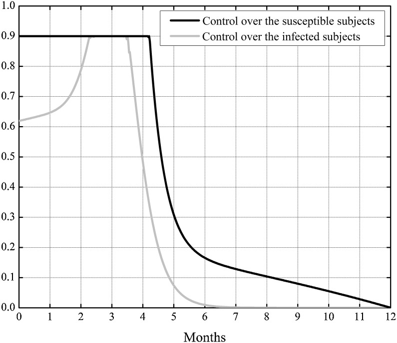
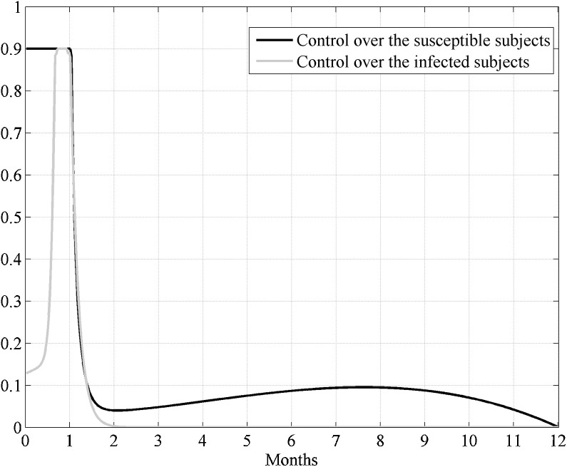
In the following this will be recalled as Case I. In Fig. 2 the two obtained controls are presented. Note that the control u, which acts directly over the susceptible, assumed its maximum value at the beginning of the control period till four months (more precisely, 126 days) and successively decreased monotonically, whereas the control v augmented to its maximum value, that reached after almost two months and a half since the beginning of the treatment, and then it decreased monotonically from the third month and a half. The control over the infected subjects could be reduced almost to zero after about 6 months since the beginning of the treatment.

Fig. 2.

Case I. The optimal controls u(t) and v(t) when the epidemic has not yet widespread.

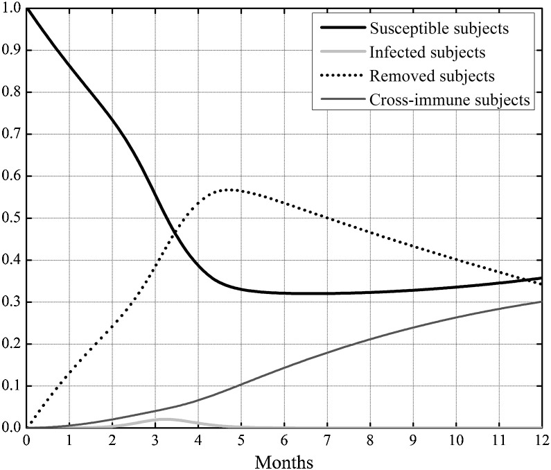
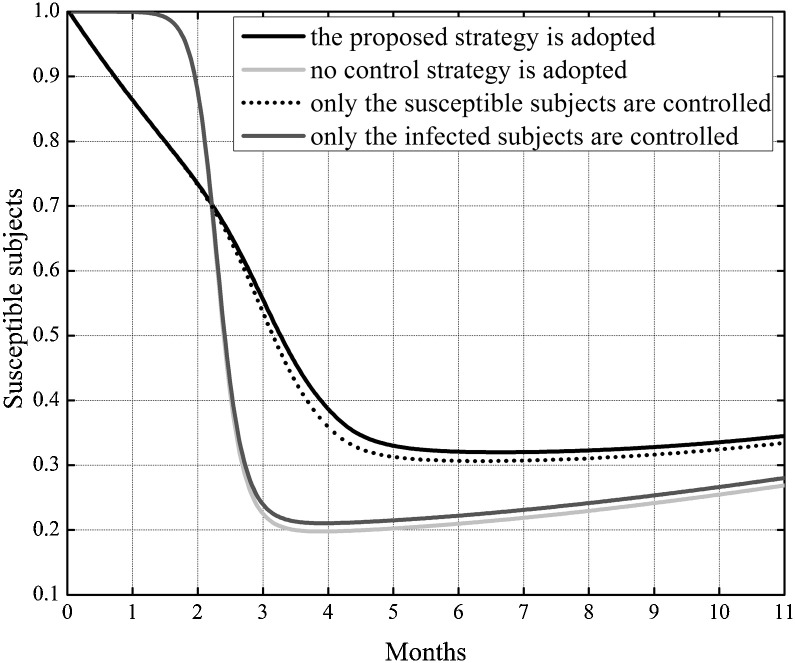
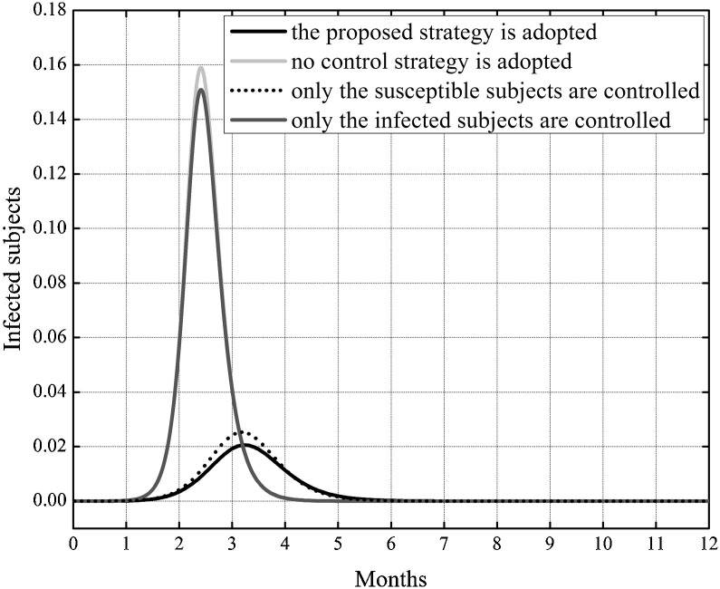
In Fig. 3 the behavior of the susceptible, infected, removed and cross immune subjects when the two optimal controls were active is shown. To check the effects of the control strategy that directly acted both on susceptible and infected subjects, the same simulation of Fig. 3 was repeated also in other three situations: assuming no control, neither on susceptible nor on the infected, assuming the control only on the susceptible and finally considering the control only on the infected. In Fig. 4, Fig. 5 the behavior of the susceptible and the infected subjects in the four analyzed situation are represented in the first eleven and twelve months of the control period, respectively. As far as the number of susceptible is concerned, its reduction with respect to the initial value S ₀ was almost equivalent both when the strategy with double control was adopted and when only the susceptible were controlled, with a value of about 65%. In absence of all control actions or in presence of control only on the infected subjects the reduction with respect to S ₀ was about 71%.

Fig. 3.

Case I. Solutions of the SIRC model using the two optimal controls.

Fig. 4.

Case I. Comparison of the incidence of the susceptible subjects in the four considered situations: assuming no control, neither on susceptible nor on the infected, assuming the control only on the susceptible, considering the control only on the infected, considering the proposed double controls.

Fig. 5.

Case I. Comparison of the incidence of infected subjects in the four considered situations assuming no control, neither on susceptible nor on the infected, assuming the control only on the susceptible, considering the control only on the infected, considering the proposed double controls.

Although the situation seems to be worse adopting the double control strategy, in Fig. 4 one can notice that the number of susceptible subjects strongly decreased at the beginning of the outbreak due to their relocation in the removed class, resulting in an important leak of potential infected people, as can be appreciated in the lower peak of epidemic and in its delay, Fig. 5.

To compare numerically the different strategies over the infected subjects, as reference situation was assumed the absence of control and the following percentage was evaluated:

$$q_I=\frac{\max (I)-\max (\overline{I})}{\max (\overline{I})}\times 100$$

where the superscript $\overline{I}$ represented the infected subjects in the reference situation of no control and I were the infected subjects in one of the considered control situations; it is a measure of the reduction of the peak of influence. The quantity q _I was equal to −87% when the double control strategy was adopted, whereas when controlling only the susceptible or only the infected the same quantity was equal to −84% and −5% respectively.

This result enhanced that the strategy that controlled both the susceptible and the infected yielded a more significant reduction in the number of infected subjects than the other control strategies.

As far as the second situation considered the following choice for the initial values was assumed:

S ₀  = 0.99, I ₀  = 5 × 10⁻³, R ₀  = 3 × 10⁻³, C ₀  = 2 × 10⁻³

In the following this will be recalled as Case II. This means that the control strategy started when the epidemic was already significantly widespread.

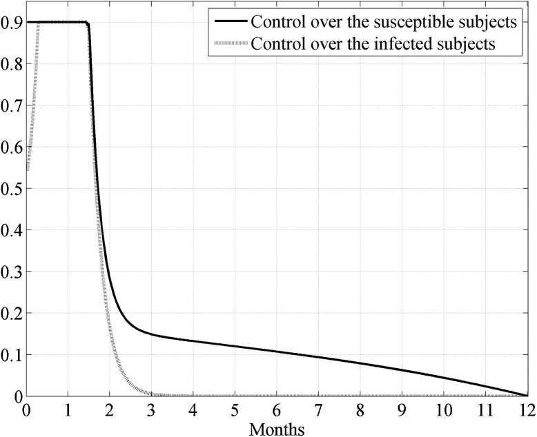
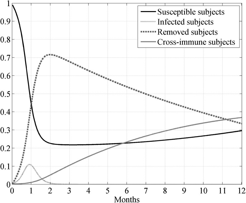
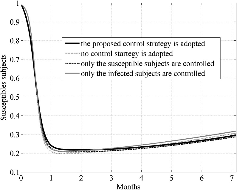
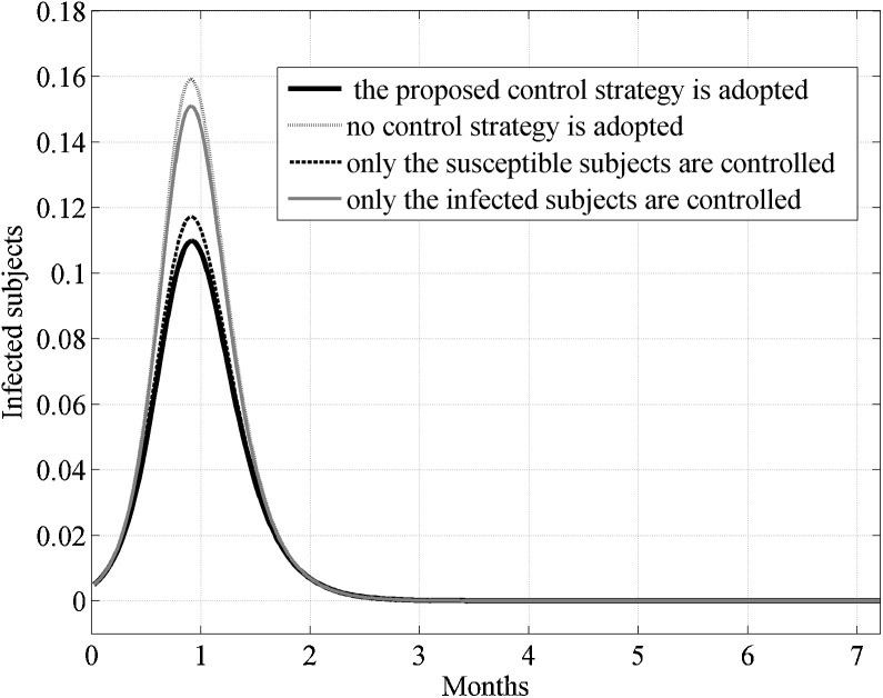
In Fig. 6 the two obtained optimal controls are presented. Note that the control u assumed its maximum value at the beginning of the control period till one month and a half (more precisely, 44 days) and successively it decreased monotonically, whereas the control v augmented to its maximum value, that reached after one week since the beginning of the treatment, and then it decreased monotonically after about one month and a half. The control over the infected subjects should be reduced almost to zero after almost four months (113 days) since the beginning of the treatment. In Fig. 7 the behavior of the susceptible, infected, removed and cross immune subjects when the two optimal controls were active is shown. Also in this situation, to check the effects of the control strategy that directly acted both on susceptible and infected subjects, the same simulation of Fig. 7 was repeated in three situations: assuming no control, assuming the control only on the susceptible and finally considering the control only on the infected. In Fig. 8, Fig. 9 the behavior of the susceptible and the infected subjects in the four analyzed situations are represented in the first seven months of the control period, respectively. As far as the number of susceptible is concerned, its reduction with respect to the initial value S ₀ was almost equivalent both when the strategy with double control was adopted and when only the susceptible were controlled, with a value of about −70%. In absence of all control actions or in presence of control only on the infected subjects the reduction with respect to S ₀ was about 67%. The effects of the control strategies over the number of infected subjects were analyzed by means of the q _I quantity. It was equal to −31% when the double control strategy is adopted, whereas, when controlling only on the susceptible and only on the infected, the same quantity was equal to −26% and −5% respectively. This result enhanced that the strategy that controlled both the susceptible and the infected yielded a more significant reduction in the number of infected subjects than the other control strategies. Moreover, note that in the Case II, the peak of epidemic did not change significantly in time, even if, as already pointed out, changed significantly in its values, depending on the chosen control strategy.

Fig. 6.

Case II. The optimal controls u(t) and v(t) when the epidemic was already significantly widespread.

Fig. 7.

Case II. Solutions of the SIRC model using the two optimal controls.

Fig. 8.

Case II. Comparison of the incidence of the susceptible subjects in the four considered situations: assuming no control, neither on susceptible nor on the infected, assuming the control only on the susceptible, considering the control only on the infected, considering the proposed double controls.

Fig. 9.

Case II. Comparison of the incidence of infected subjects in the four considered situations assuming no control, neither on susceptible nor on the infected, assuming the control only on the susceptible, considering the control only on the infected, considering the proposed double controls.

In both cases it is interesting to study the influence of the reproduction number (and therefore of the transmission parameter β) on the optimal control strategy. Note that this parameter influences not only the contact rate of susceptible subjects, but also the possibility of re-entering in the removed compartment after the cross-immune period. Two new situations were considered: a reproduction number equal to 6 and to 10, i.e. equal to the half and end point of the allowed range. In Case I, for $\overline{R}=6$ it was noted that the control u(t) started from the maximum value allowed and decreased at day 21, whereas the control over the infected reached the maximum value at day 16, decreasing after 2 weeks. Similar results may be observed for $\overline{R}=10$, with the control over the susceptible that began to decrease from the maximum value after 13 days and the control over the infected that assumed the maximum value between the day eleven and twenty-three, and then decreases.

In the case of $\overline{R}=6$, as far as the number of susceptible is concerned, its reduction with respect to the initial value S ₀ was about of 85%; this value, larger that the corresponding one obtained with $\overline{R}=2$, is reasonable since the contact rate is greater. The effects of the control strategies over the number of infected subjects was analyzed by means of the q _I quantity that was equal to −15%, thus enhancing a less evident reduction of the number of infected subjects, than in the previous situation; also the peak location, that came earlier (about after three weeks), reflected the influence of the larger contact rate. The same considerations hold also in the case of $\overline{R}=10$, in which the reduction of the number of susceptible individuals with respect to the initial value S ₀ was almost constant whereas the q _I quantity was equal to −7% and also the peak was located significantly earlier (day 14).

Similar considerations hold also for the Case II of an epidemic already significantly widespread. As far as the control is concerned, for $\overline{R}=6$ the control over the susceptible subjects, starting from the maximum value allowed, began to decrease at day 10, whereas the control over the infected reached the maximum value at day 5 and began to decrease after about 3 weeks (20 days). Again, the optimal solution was a maximum effort at the beginning of the disease, and successively decreased. Similar results could be observed for $\overline{R}=10$, with the control over the susceptible that began to decrease from the maximum value after about a week and the control over the infected that assumed the maximum value between the day four and sixteen, and then decreased. Both for $\overline{R}=6$ and $\overline{R}=10$ the reduction of the number of susceptible subjects with respect to the initial value S ₀ was about of 85%, thus confirming the behavior of Case I. Even more evident was the change in the location of the peak of the epidemic, being at about day 7 and 5 respectively, with a quantity q _I equal to −5.68% and −3.02% for the two choices of the reproduction number, thus denoting the effects of an epidemic with a contact rate really significant and the limit of the control strategy with the chosen control parameters, in the case of an epidemic already widespread and a control action not as effective as it could be in the Case I.

3.1. Control parameters sensitivity analysis

It is interesting to analyze in Case I and Case II, with $\overline{R}=2$, the influence of the weighting parameters α ₁,α ₂, τ ₁,τ ₂  > 0 in the cost index and ρ ₁,ρ ₂  > 0 in the controls. More precisely, assuming as reference case the values (23) for α ₁,α ₂, τ ₁,τ ₂  > 0 and ρ ₁  =  ρ ₂  = 2, the situations summarized in Table 1, Table 2 were considered.

Table 1.

Case I. Control parameters sensitivity analysis.

Case I S0 = 1 − I0, I0 = 10−6, R0 = 0, C0 = 0
	$\frac{S(\text{end})-S_0}{S_0}$	qI	Location of the peak of the epidemic spread (days)
Reference case: α1 = 10−3, α2 = 0.997, τ1 = 10−3, τ2 = 10−3, ρ1 = 2, ρ2 = 2	−64%	−87%	97
α1 = 0.298, α2 = 0.7, τ1 = 10−3, τ2 = 10−3, ρ1 = 2, ρ2 = 2	−89%	−0.8%	72
α1 = 10−3, α2 = 0.997, τ1 = 0.0005 = 1/3τ2, ρ1 = 2, ρ2 = 2	−67%	−86%	96
α1 = 10−3, α2 = 0.997, τ1 = 0.0015 = 3τ2, ρ1 = 2, ρ2 = 2	−62%	−87%	98
α1 = 10−3, α2 = 0.997, τ1 = 10−3, τ2 = 10−3, ρ1 = 10, ρ2 = 1	−85%	−99%	33
α1 = 10−3, α2 = 0.997, τ1 = 10−3, τ2 = 10−3, ρ1 = 1, ρ2 = 10	−60%	−70%	94

Table 2.

Case II. Control parameters sensitivity analysis.

Case II S0 = 0.99, I0 = 5×10−3, R0 = 3×10−3, C0 = 2×10−3
	$\frac{S(\text{end})-S_0}{S_0}$	qI	Location of the peak of the epidemic spread (days)
Reference case: α1 = 10−3, α2 = 0.997, τ1 = 10−3, τ2 = 10−3, ρ1 = 2, ρ2 = 2	−70%	−31%	28
α1 = 0.298, α2 = 0.7, τ1 = 10−3, τ2 = 10−3, ρ1 = 2, ρ2 = 2	−88%	−0.8%	27
α1 = 10−3, α2 = 0.997, τ1 = 0.0005 = 1/3τ2, ρ1 = 2, ρ2 = 2	−72%	−31%	28
α1 = 10−3, α2 = 0.997, τ1 = 0.0015 = 3τ2, ρ1 = 2, ρ2 = 2	−69%	−31%	28
α1 = 10−3, α2 = 0.997, τ1 = 10−3, τ2 = 10−3, ρ1 = 10, ρ2 = 1	−84%	−79%	21
α1 = 10−3, α2 = 0.997, τ1 = 10−3, τ2 = 10−3, ρ1 = 1, ρ2 = 10	−63%	−38%	29

In the case in which the epidemic has not yet widespread if the ratio between the weights α ₁,α ₂, was about 0.40 (and not 0.001 as in the case already examined) the final number of susceptible subjects decreased of a percentage of about 89% with respect to the initial value, but with a control effort in the prevention that should be equal to the maximum value allowed u _max  = 0.9 for almost all the control interval. Moreover the peak of the infected subjects slightly decreased of about 0.8%.

As far as the influence of the weights τ ₁,τ ₂  > 0, two situations were compared to the reference case. In the first one τ ₁, the weight of the control over the susceptible subjects, was assumed equal to 1/3 of the weight τ ₂; this allowed a more significant effort in the prevention showing a decrease of susceptible subjects of about 67%, and a significant decrease of 86% could be appreciated for the peak of the infected ones. In the second situation considered the weight τ ₁ was assumed three times larger than the weight τ ₂; in this case the number of susceptible decreased of about 62% with a decrease of the peak of epidemic of about 87%.

As far as the influence of the parameters ρ ₁,ρ ₂  > 0 is concerned, when ρ ₁  = 10, ρ ₂  = 1 it is interesting to note the reduction of the susceptible subjects of about 85% with respect to the initial value, with a very significant reduction of the peak of epidemic (99%) that was located after about one month (33 days). When ρ ₁  = 1, ρ ₂  = 10 it is worth noting the delay of the peak of influence, about three months (94 days), with a reduction of 70%; the reduction of the susceptible subjects with respect to the initial value was of 60%.

In Case II, the case of control strategies acting only when epidemic has already widespread, when α ₁  = 0.4α ₂ the final number of susceptible subjects decreased of about 88%, with a control effort in the prevention that should be equal to the maximum value allowed for almost all the control interval. Moreover the peak of the infected subjects slightly decreased (about 0.8%), as in the previous case of well-timed control strategy.

As far as the influence of the weights τ ₁,τ ₂  > 0, in the first case considered, τ ₁  = 1/3τ ₂, a more significant effort in the prevention was allowed showing a decrease of susceptible subjects of about 72%, whereas no significant differences could be appreciated for the infected ones. When τ ₁  = 3τ ₂ the number of susceptible decreased of about 69% with a decrease of the peak of epidemic of about 30%.

Note that in all these cases analyzed, when the control effort started only with the epidemic already diffused, the temporal location of the peak of the epidemic spread did not change significantly with respect to the non-control case, whereas if the control effort is well-timed the location of the peak of the epidemic spread is significantly delayed.

As far as the influence of the parameters ρ ₁,ρ ₂  > 0 is concerned, when ρ ₁  = 10, ρ ₂  = 1 it is interesting to note the reduction of the susceptible subjects of about of 84% with respect to the initial value, with a significant reduction of the peak of epidemic (79%) that was temporally located at day 21. When ρ ₁  = 1, ρ ₂  = 10 it is worth noting the delay of the peak of influence (about one month) with a reduction of 38%, whereas the reduction of the susceptible subjects was of 63% with respect to the initial value.

It is worth noting the more evident effectiveness of the optimal control strategy when it was well-timed, with respect to the situation in which the control effort acted on the epidemic already spread out. In the first case the action on susceptible and infected subjects allowed an increase of the number of removed subjects, yielding a delay in the peak of influence that was significantly reduced.

The same analysis of Table 1, Table 2 were performed also in the case of $\overline{R}=6$ and $\overline{R}=10$. As it was to be expected, in Case I for $\overline{R}=6$ the control parameters that yielded the most significant reduction of the peak of influence were α ₁  = 10⁻³, α ₂  = 0.997, τ ₁  = 10⁻³, τ ₂  = 10⁻³, ρ ₁  = 10, ρ ₂  = 1, obtaining a value of q _I equal to −60% and a reduction of the susceptible subjects of 88% with respect to the initial value. For $\overline{R}=10$, using the same set of parameter, a q _I  = −37% and a reduction of the number of susceptible subjects of about 88% can be obtained.

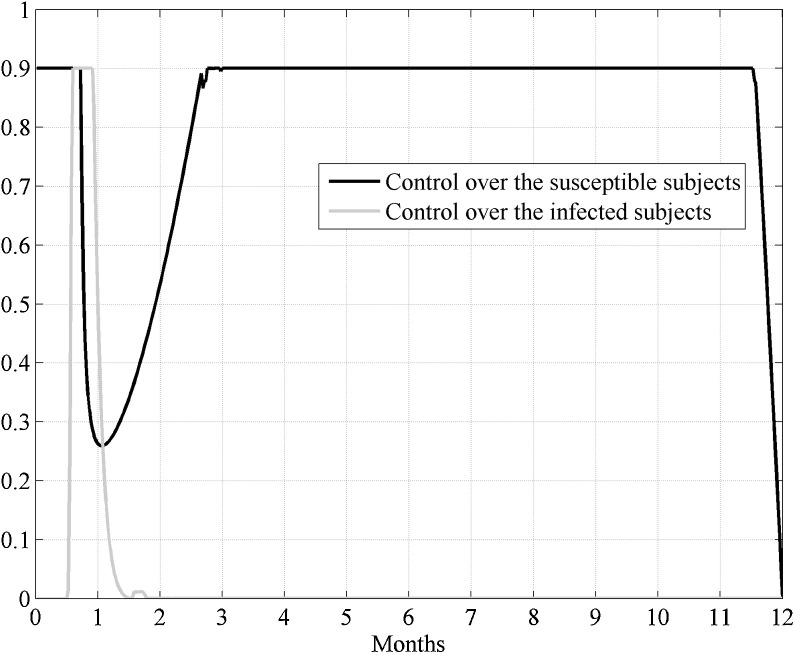
Also in Case II, when the control acted over an epidemic already widespread, for $\overline{R}=6$ the more evident percentage reduction of the peak of influence (q _I) at about day 10 was of 22% when ρ ₁  = 10, ρ ₂  = 1 and the other parameters equal to the reference case (23); for this choice there was also a significant reduction of the susceptible subjects with respect to the initial value (−87%). The same results were obtained also for $\overline{R}=10$, with a q _I equal to −12% and a location of the peak of influence after a week of the beginning of the control period. These results (Case I and II for $\overline{R}=6$ and $\overline{R}=10$) were reasonable, since in the cost index it was privileged the minimization over the number of susceptible subjects. It is particularly interesting the behavior of the control over the susceptible: after a first decreasing period (about 40 days) it increased again, see Fig. 10 as an example of Case I, $\overline{R}=6$. This is due increased contact rate that requested an additional control.

Fig. 10.

Case I. Analysis of the influence of the reproduction number on the control strategy, when $\overline{R}=6$ and ρ₁ = 10, ρ₂ = 1.

Even more evident is the same behavior of the control u in the case in which α ₁  = 0.4α ₂ (and the other parameters equal to the reference case (23)), as already noted in the case $\overline{R}=2$, see Fig. 11 ; this is because the control u needed an extra effort to reduce the number of susceptible subjects, as requested by the cost index. It is worth noting that in these cases (Cases I and II, α ₁  = 0.4α ₂) the reduction of the number of infected subjects was not, obviously, as effective as in the reference case.

Fig. 11.

Case I. Analysis of the influence of the reproduction number on the control strategy, when $\overline{R}=6$ and α₁ = 0.4α₂.

4. Conclusions

In this paper the SIRC model of influenza is considered aiming at the control of the epidemic spreading; controlling an epidemic disease corresponds, for example, to an ad hoc introduction of vaccine or quarantine or medicine treatment strategy. All the possible strategies should face with the limitations of the resource. In this paper the controls both in the susceptible and in the infected classes are introduced, taking into account the constraints in the controls. A suitable cost index is proposed and existence result is assessed. The aim is to minimize the susceptible and infected subjects with as less resources as possible; the analytical expressions of the optimal controls are provided and their numerical implementation is discussed. Numerical results are presented comparing the effects of different control strategies, showing interesting and encouraging results.

References

- 1.Hethcote H., Zhien M., Shengbing L. Effects of quarantine in six endemic models for infectious diseases. Mathematical Biosciences. 2002;180:141–160. doi: 10.1016/s0025-5564(02)00111-6. [DOI] [PubMed] [Google Scholar]
- 2.Casagrandi R., Bolzoni L., Levin S.A., Andreasen V. The SIRC model and influenza A. Mathematical Biosciences. 2006;200:152–169. doi: 10.1016/j.mbs.2005.12.029. [DOI] [PubMed] [Google Scholar]
- 3.Becker N.G., Starczak D.N. Optimal vaccination strategies for a community of household. Mathematical Biosciences. 1997;139:117–132. doi: 10.1016/s0025-5564(96)00139-3. [DOI] [PubMed] [Google Scholar]
- 4.Brandeau M., Zaric G.S., Richter A. Resource allocation for control of infectious diseases in multiple independent populations: beyond cost-effectiveness analysis. Journal of Health Economics. 2003;22:575–598. doi: 10.1016/S0167-6296(03)00043-2. [DOI] [PubMed] [Google Scholar]
- 5.Castilho C. Optimal control of an epidemic through educational campaign. Electronic Journal of Differential Equations. 2006;125:1–11. [Google Scholar]
- 6.Zaric G.S., Brandeau M. Dynamic resource allocation for epidemic control in multiple populations. Journal of Mathematics Applied in Medicine and Biology. 2002;19:235–255. [PubMed] [Google Scholar]
- 7.Verriest E., Delmotte F., Egerstedt M. Control of epidemics by vaccination. Proceedings of the American Control Conference. 2005;2:985–990. [Google Scholar]
- 8.Clancy D., Piunovskiy A.B. An explicit optimal isolation policy for a deterministic epidemic model. Applied Mathematics and Computation. 2005;163:1109–1121. [Google Scholar]
- 9.Behncke H. Optimal control of deterministic epidemics. Optimal Control, Applications and Methods. 2000;21:269–285. [Google Scholar]
- 10.Becker N.G., Glass K., Li Z., Aldis G.K. Controlling infectious diseases like SARS. Mathematical Biosciences. 2005;193:205–221. doi: 10.1016/j.mbs.2004.07.006. [DOI] [PubMed] [Google Scholar]
- 11.Jiang C., Dong M. Optimal measures for SARS epidemics outbreaks. Proc. of the 6th World Congress on Intelligent Control and Automation; Dalian, China; 2006. pp. 9331–9335. [Google Scholar]
- 12.Chang H., Astolfi A. Enhancement of the immune system in HIV dynamics by output feedback. Automatica. 2009;45:1765–1770. [Google Scholar]
- 13.Caetano M.A.L., Yoneyama T. Optimal and sub-optimal control in Dengue epidemics. Optimal Control, Applications and Methods. 2001;22:63–73. [Google Scholar]
- 14.Yan X., Zou Y. Optimal and suboptimal quarantine and isolation control in SARS epidemics. Mathematical and Computer Modelling. 2008;47:235–245. doi: 10.1016/j.mcm.2007.04.003. [DOI] [PMC free article] [PubMed] [Google Scholar]
- 15.Joshi H. Optimal control of an HIV immunology model. Optimal Control, Applications and Methods. 2002;23:199–213. [Google Scholar]
- 16.Iacoviello D., Liuzzi G. Fixed/free final time SIR epidemic models with multiple controls. International Journal of Simulation and Modelling. 2008;7:81–92. [Google Scholar]
- 17.Jung E., Lenhart S., Feng Z. Optimal control of treatment in a two strain tuberculosis model. Discrete and Continuous Dynamical Systems – Series B. 2002;2:473–482. [Google Scholar]
- 18.Blayneh K., Cao Y., Kwon H.D. Optimal control of vector-borne diseases: treatment and prevention. Discrete and Continuous Dynamical Systems – Series B. 2009;11:1–30. [Google Scholar]
- 19.Anderson R., May R. Population biology of infectious diseases: Part I. Nature. 1979:280–361. doi: 10.1038/280361a0. [DOI] [PubMed] [Google Scholar]
- 20.Pease C. An evolutionary epidemiological mechanism, with applications to type A influenza. Theoretical Population Biology. 1987;31:422–452. doi: 10.1016/0040-5809(87)90014-1. [DOI] [PubMed] [Google Scholar]
- 21.Zaman G., Kang Y.H., Jung I.H. Stability analysis and optimal vaccination of an SIR epidemic model. BioSystems. 2008;93:240–249. doi: 10.1016/j.biosystems.2008.05.004. [DOI] [PubMed] [Google Scholar]
- 22.Birkhoff G., Rota G.C.C. 4th ed. John Wiley & Sons; New York: 1989. Ordinary Differential Equations. [Google Scholar]
- 23.Fleming W.H., Rishel R.W. Springer Verlag; New York: 1975. Deterministic and Stochastic Optimal Control. [Google Scholar]
- 24.Lukes D.L. vol. 162. Academic Press; New York: 1982. (Differential Equations: Classical to Controlled. Mathematics in Science and Engineering). [Google Scholar]
- 25.Hartl R.F., Sethi S.P., Vickson R.G. A survey f the maximum principles for optimal control problems with state constraints. Society for Industrial and Applied Mathematics. 1995;37:181–218. [Google Scholar]
- 26.Fletcher R. John Wiley and Sons; UK: 1987. Practical Methods of Optimization. [Google Scholar]
- 27.Gill P.E., Murray W., Wright M.H. Academic Press; London: 1981. Practical Optimization. [Google Scholar]
- 28.Battiti R. First and second order methods for learning: between steepest descent and Newton's method. Neural Computation. 1992;4:141–166. [Google Scholar]
- 29.Lenhart S., Workman J.T. Chapman & Hall/CRC; London, UK: 2007. Optimal Control Applied to Biological Models, Mathematical and Computational Biology Series. [Google Scholar]