

Abstract
Within the standard SIR model with spatial structure, we propose two models for the superspreader. In one model, superspreaders have intrinsically strong infectiousness. In other model, they have many social connections. By Monte Carlo simulation, we obtain the percolation probability, the propagation speed, the epidemic curve, the distribution of secondary infected and the propagation path as functions of population and the density of superspreaders. By comparing the results with the data of SARS in Singapore 2003, we conclude that the latter model can explain the observation.
Keywords: SARS, Superspreader, SIR model, Epidemic model
1. Introduction
Severe acute respiratory syndrome (SARS) was first identified in Guangdong, China, in November 2002. During the next few months, SARS spread through Asia, Europe, North and South America. More than 8000 people worldwide were infected during the 2003 outbreak, and more than 700 people died [1]. It is now believed that the sharp increase and decrease in the number of patients was caused by the existence of superspreaders. According to Centers for Disease Control and Prevention (CDC) of the USA, the patients are defined as superspreaders if they infect more than 10 people [2]. Superspreaders thus have a strong effect on other people and cause wide spread of the disease. Although superspreaders are believed to play important roles in the outbreak of SARS, the biological characterization of the superspreaders have not been performed.
Standard mathematical models of the spread of infectious diseases are well known and have been widely applied for many diseases [3]. In the standard model (SIR model), individuals are categorized into three groups; susceptible to the disease (S), infected with the disease (I), or recovered (R). The evolution of these states is described by difference (or differential) equations and it is assumed that the transmission rates between all pair of individuals are equal. In order to include the effect of a superspreader, the SIR model must be generalized so that the transmission rates can represent the effect of superspreaders.
The cases in Hong Kong and Singapore are reported as the super spreading events of SARS. Up to now, to reproduce these cases, a variety of mathematical models were suggested. Although Lipsitch et al. consider the superspreaders to be exceptional [4] and Riley et al. do not directly adopt them [5]. Masuda et al. used the network model as the model which incorporates the superspreaders directly [6]. We introduce the superspreader as an important key directly into the model, and try the reproduction of the spread of SARS by using a simplified model.
In this paper, we investigate the SIR model in two-dimensional continuous space where the infection probability has a dependence of the distance between the two individuals, and the difference of normal and superspreader individuals is implemented in this dependence. First we assume that a normal infected individual transmits his/her disease to a susceptible individual at distance with probability in proportion to if and zero if , where . We consider two models for the superspreaders. In one model, the superspreader can transmit the disease with higher probability to other people within the same distance. In the other model, the superspreader can transmit disease to susceptible people at much longer distance. These models can be called the strong infectiousness model and the hub model, respectively. By Monte Carlo simulation, we investigate the spread of disease as a function of population and the density of superspreaders. In Section 2, we explain our model in detail. In Section 3, results of Monte Carlo simulation are presented about the percolation probability of disease, the velocity of disease propagation, the epidemic curve and secondary infections. We compare our results with observation for the SARS outbreak in 2003 in Section 4. We conclude that the hub model can explain the observation.
2. Models
We consider N individuals distributed on an continuous space whose positions are fixed. We impose periodic boundary conditions. An initial-infected individual is placed on the bottom of the system, and remaining individuals are placed randomly on the space. Each individual is in one of three possible state; susceptible (S), infected (I) and recovered (R). In one Monte Carlo step, first an infected individual is chosen randomly, and it infects all susceptible individuals with probability . Here is the infection probability which depends on the distance between the two individual. The susceptible individuals which are infected change into a new infected individual. At the same time, the infected individual changes into the recovered with recovery probability . We carry out a sequence of these operations for all infected individuals without new infected ones.
Superspreaders are mixed in normal individuals group, whose fraction is denoted by . We characterize the normal individuals and the superspreaders through the infection probability . In this paper, we investigate two models for the superspreader.
2.1. Strong infectiousness model
Let the normal infection probability be a decreasing function of distance r with cutoff . In this model, the superspreader is assumed to have strong infectiousness intrinsically. Thus, we assume that its infection probability of a superspreader has the same cutoff as normal ones, and it is not a decreasing function of distance r but constant. Namely, is assumed as
| (1) |
We set for the normal infection probability and for superspreaders (Fig. 1 ).
Fig. 1.

The distance dependence of infection probability in the strong infectiousness model. The superspreader's is constant (solid line), and the normal's is a decreasing function (dashed line). Both species have the same cutoff.
2.2. Hub model
Let the normal infection probability be the same function as the strong infectiousness model. In this model, the superspreader is assumed to make more social contacts with other people than normal individuals. Therefore, we assume that superspreader's infection probability is the same functional form, but it has a longer cutoff than normal's cutoff. is defined as
| (2) |
We set for the normal infection probability and for the superspreaders. In order to compare essential difference between these two models, we normalize two models so that the infection rate for both models are equal. Because of the factor in the hub model, the numbers of infected individuals which are infected by a superspreader per unit time are equal for the strong infectiousness model and for the hub model (Fig. 2 ).
Fig. 2.

The distance dependency of infection probability in the hub model. The normal's (dashed line) and the superspreader's (solid line) is the same functional form which is a decreasing function. The normal's cutoff is , and the superspreader's cutoff is .
3. Results
Monte Carlo simulation was performed from to on continuous space with , and is fixed to , . We obtained the various quantities by averaging over 1000 Monte Carlo runs whose initial positions are changed.
3.1. Percolation probability
When infection which started at the bottom of the system reaches on the top of it, we regard this trial as percolated, and define the percolation probability as the ratio of percolated trials to total trials.
Figs. 3 and 4 show the dependence of the percolation probability on the density for several values of . We can see the percolation transition on both models for all values of . At low density, the infection does not percolate, in other words, the disease stops before spreading to the whole system. On the other hand, at the high density, the infection percolates and the disease spreads the whole system. As is increased the critical density shifts to the lower density and the transition becomes sharper.
Fig. 3.

The percolation probability as a function of the density for different in the strong infectiousness model.
Fig. 4.
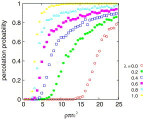
The percolation probability as a function of the density for different in the hub model.
Fig. 5 shows the dependence of the critical density on the fraction of superspreaders . The parameter space above the critical line is the area where the disease percolates on, the other side is the area where the disease does not percolate. In order to explain the decrease of the critical density , we introduce the basic reproductive number which is defined as
| (3) |
Here and are the infection probability of the superspreaders and the normal individuals, respectively. This quantity denotes the mean of the number of new infected individuals per unit time resulting from a single initial-infected individual. In the strong infectiousness model, if all individuals are superspreaders, the critical density is determined by theory of percolation [7], and we define the critical basic reproductive number as
| (4) |
In the hub model, we choose the critical density where as the critical basic reproductive number,
| (5) |
The solid and dashed curves in Fig. 5 are critical curves defined by the condition . We can see coincidence between the boundary lines of and the critical density .
Fig. 5.

Dependence of critical density on parameter . The critical lines show . The circles and solid line are in the strong infectiousness model, and the squares and dashed line are in the hub model. Above the critical curves, the disease percolates, and below the curves, the disease does not percolate.
3.2. Propagation speed
We define the velocity of propagation as the velocity of front line. Let be the distance between the initial infected individual and the furthest infected individual from it. The time dependence of the distance for six different values is shown in Fig. 6 .
Fig. 6.

The time evolutions of the distance between the initial-infected individual and front line of propagation for different in the strong infectiousness model.
Before reaches its plateau due to the boundary, we define the velocity of propagation by the first order differential coefficient with respect to time.
Fig. 7 shows the dependence of the velocity of propagation on the fraction of superspreaders for . We can see the velocity is an increasing function of , and the velocity in the hub model is larger than in the strong infectiousness model for any .
Fig. 7.

The velocity of propagation as a function of for two models. The circles are in the strong infectiousness model, and the squares are in the hub model.
3.3. Epidemic curve
Fig. 8 shows the influence of the superspreaders of both models on the number of newly infected individuals as a function of time (epidemic curves).
Fig. 8.

Epidemic curves (the number of newly infected individuals per timestep) for different models. The circles are in the strong infectiousness model, and the squares are in the hub model where and . The triangles are the epidemic curves when no superspreaders exact .
It can be seen that the number of newly infected individuals with superspreaders of the hub model increases rapidly and the maximum appears at a shorter time than in the case for the strong infectiousness model and in the case without superspreaders.
3.4. Distribution of secondary infected
We consider the network of the infection route after the infection is terminated. Figs. 9–11 show the network of the infection route for the strong infectiousness model, the hub model and those without superspreaders.
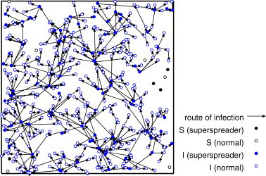
Fig. 9.
The route of infection on the strong infectiousness model where and .
Fig. 11.
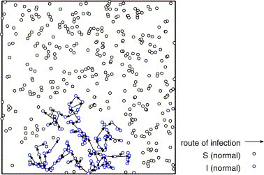
The route of infection where and .
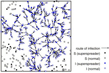
From Fig. 9 , we can see that some superspreaders infect the large number of individuals locally, and the most of normal individuals infect none or a few individuals (at most two or three individuals) in the strong infectiousness model. Fig. 10 shows that there are some long paths of infection from superspreaders to other individuals in the hub model. These long paths are the origin of high velocity of propagation. In Fig. 11 , the infection stops on the way and does not percolate because of low density. The distribution of the number of links of these networks corresponds to the distribution of secondary infected.
Fig. 10.
The route of infection on the hub model where and .
Fig. 12 shows the distribution of the number of links of the network formed by spreading on the system without superspreaders, and Fig. 13 shows the distributions of them in the case with superspreaders on both models.
Fig. 12.

Distribution of the number of links on the network after influence where (i.e., no superspreader exist) and .
Fig. 13.

Distribution of the number of links on the network after influence on both models for the superspreaders where and .
If superspreaders are mixed in the system, we can see from Fig. 13 that both models give similar distributions. Comparing with Fig. 12, the features of the distributions in Fig. 13 are that their distributions at zero is much larger than other number of links and that they have long tails.
4. Comparison with the data of SARS
Fig. 14 shows the number of direct secondary patients from probable cases of SARS in Singapore from February 25 to April 30, 2003 [2].
Fig. 14.
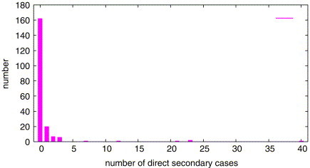
Number of direct secondary patients from SARS (Singapore, February 25–April 30, 2003).
The SARS patients which infect 12, 21, 23 and 40 persons are superspreaders. The feature of this distribution is similar with the distributions from our models shown in Fig. 13. Therefore, our models are in line with these observations for SARS.
We also show in Fig. 15 the epidemic curve (the histogram) of SARS in Singapore from February 13 to June 13, 2003 [8].
Fig. 15.

Epidemic curves of SARS (Singapore, February 13–June 13, 2003) and comparison with the results of our models. The circles are for the strong infectiousness model, and the squares are for the hub model where . The triangles are no superspreaders . The number of initial susceptible individuals N is () and 1 timestep is fitted to 6 days.
Comparing with the results of our models, we conclude that it is more similar to the hub model where parameters are given as , and . It suggests that the superspreader of SARS spread the infection in a way like the hub model, in other words, the superspreader is a person having many social connections.
5. Conclusions
In this paper, we have studied the effect of superspreaders in spread of epidemics. We introduced two models for superspreaders who have two kinds of distance dependence of infection probability. From Monte Carlo simulation, we have obtained the percolation probability as functions of the density for different fraction of superspreaders . If is sufficiently low, the percolation probability is zero and the percolation transition appears at the critical density . We showed the critical density decreases as increases, and coincides with the density at the critical basic reproductive number . We could see the critical density of the strong infectiousness model is larger than the hub model, and in the hub model infection propagates faster than in the strong infectiousness model for any . Moreover, the epidemic curves were shown that the number of infected increases rapidly with a sharp maximum if superspreaders are mixed in the system. With mixing the superspreaders, the distribution of the number of links of the infection route network have long tail and get enhanced at zero in comparison with no superspreaders. Our results were compared with the data of SARS outbreak in 2003. The feature of distribution of the number of secondary patients is similar with the distributions from our models. This result suggests that our models can be applied to simulate SARS. Moreover, from the comparison of the epidemic curve of SARS with our models, the hub model reproduces the epidemic curve similar to the data of SARS. From this result, we conclude that the social connections are important for the spreading of disease, and the superspreader has many social connections.
References
- 1.World Health Organization, Cumulative number of reported probable cases of severe acute respiratory syndrome (SARS), World Health Organization, 2003, http://www.who.int/csr/sars/country/en.
- 2.Centers for Disease Control and Prevention, Severe Acute Respiratory Syndrome—Singapore, 2003, MMWR 52, pp. 405–411.
- 3.Anderson R.M., May R.M. Oxford University Press; Oxford: 1991. Infectious Diseases of Humans, Dynamics and Control. [Google Scholar]
- 4.Lipsitch M., Cohen T. Science. 2003;300:1966–1970. doi: 10.1126/science.1086616. [DOI] [PMC free article] [PubMed] [Google Scholar]
- 5.Riley S., Fraser C., Donnelly C.A. Science. 2003;300:1961–1966. doi: 10.1126/science.1086478. [DOI] [PubMed] [Google Scholar]
- 6.Masuda N., Konno N., Aihara K. Phys. Rev. E. 2004;69:031917. doi: 10.1103/PhysRevE.69.031917. [DOI] [PubMed] [Google Scholar]
- 7.Pike G.E., Seager C.H. Phys. Rev. B. 1974;10:1421–1434. [Google Scholar]
- 8.World Health Organization, Epidemic curves—severe acute respiratory syndrome (SARS), World Health Organization, 2003, http://www.who.int/csr/sars/epicurve/epiindex/en/.