Generalized reproduction numbers, sensitivity analysis and critical immunity levels of an SEQIJR disease model with immunization and varying total population size

Abstract

An SEQIJR model of epidemic disease transmission which includes immunization and a varying population size is studied. The model includes immunization of susceptible people (S), quarantine (Q) of exposed people (E), isolation (J) of infectious people (I), a recovered population (R), and variation in population size due to natural births and deaths and deaths of infected people. It is shown analytically that the model has a disease-free equilibrium state which always exists and an endemic equilibrium state which exists if and only if the disease-free state is unstable. A simple formula is obtained for a generalized reproduction number $R_g$ where, for any given initial population, $R_g<1$ means that the initial population is locally asymptotically stable and $R_g>1$ means that the initial population is unstable. As special cases, simple formulas are given for the basic reproduction number $R_0$, a disease-free reproduction number $R_{df}$, and an endemic reproduction number $R_{en}$. Formulas are derived for the sensitivity indices for variations in model parameters of the disease-free reproduction number $R_{df}$ and for the infected populations in the endemic equilibrium state. A simple formula in terms of the basic reproduction number $R_0$ is derived for the critical immunization level required to prevent the spread of disease in an initially disease-free population. Numerical simulations are carried out using the Matlab program for parameters corresponding to the outbreaks of severe acute respiratory syndrome (SARS) in Beijing, Hong Kong, Canada and Singapore in 2002 and 2003. From the sensitivity analyses for these four regions, the parameters are identified that are the most important for preventing the spread of disease in a disease-free population or for reducing infection in an infected population. The results support the importance of isolating infectious individuals in an epidemic and in maintaining a critical level of immunity in a population to prevent a disease from occurring.

1. Introduction

The SEQIJR model (see, e.g., [[6], [8], [9]]) is a generalization of the well-known SEIR model of an infectious disease in which a population at risk is separated into the four categories of susceptible ($S$), exposed ($E$), infectious ($I$) and recovered ($R$) (see, e.g., [[1], [12], [27], [29]]). A susceptible person is an uninfected person who can be infected through contact with an infectious or exposed person, an exposed person is someone who has come into contact with an infectious person but is asymptomatic, an infectious person is symptomatic, and a recovered person is someone who has recovered from the disease. It is assumed that a recovered individual cannot become infected again. In an SEQIJR model, two extra categories of quarantined ($Q$) and isolated ($J$) are added to the SEIR model. A quarantined person is an exposed person who is removed from contact with the general population and an isolated person is an infectious person who is removed from contact with the general population, usually by being admitted to a hospital. Quarantine and isolation are important in controlling epidemics because they are effective methods of reducing the contact between infected and susceptible populations.

In this paper, we consider a generalization of the basic SEQIJR model developed by Gumel et al. [6] for the severe acute respiratory syndrome (SARS) outbreaks of November 2002–July 2003. The SEQIJR model of Gumel et al. for the SARS outbreaks is useful for study for several reasons. Firstly, Gumel et al. suggested parameter values which can be used to obtain physically reasonable models for the four SARS outbreaks in Beijing, Hong Kong, Singapore and Toronto. Secondly, considerable data are available on the SARS outbreaks and mathematical models and the effectiveness of control measures have been studied by many authors (see, e.g., [[3], [7], [11], [13], [17], [18], [19], [20], [21], [26], [30]]).

In building their model, Gumel et al. assumed that there was no immunization (no vaccine was available for SARS), that susceptible people were born into the community at a constant rate and that the population was constant. They analyzed the effects of quarantine and isolation on the transmission of SARS and showed that an effective isolation policy was more important than quarantine or a combination of quarantine and a less effective isolation policy in reducing the transmission of the disease. A similar conclusion was obtained by Koonprasert et al. [9] in a numerical study of the effectiveness of quarantine and isolation. However, as noted by a number of authors (see, e.g., [[4], [5], [14], [15], [24], [28]]), the effectiveness of isolation requires strict hospital hygiene to reduce the hospital-based (nosocomial) spread of a disease.

The modifications introduced in our analysis include: (1) the existence of an immunization program, (2) changes in the total population due to births and deaths, (3) the derivation of generalized reproduction numbers for disease-free states and endemic equilibrium states, (4) a sensitivity analysis of the effect of variations in parameter values on the reproduction numbers for disease-free states and on the infected populations of the endemic equilibrium state, and (5) a derivation of a simple formula for the critical immunization level required to prevent spread of the disease in an initially disease-free population.

The organization of the paper is as follows. In Section 2, we define the mathematical model. In Section 3, we obtain analytical formulas for disease-free and endemic equilibrium points. Section 4 contains an analysis of the local stability of the equilibrium points and gives derivations of formulas for the generalized reproduction numbers. Formulas are derived for sensitivity indices in Section 5 and for critical immunization levels in Section 6. Section 7 and 8 contain results of numerical simulations using Matlab for the parameter values proposed by Gumel et al. [6] for four of the cities affected by the SARS outbreaks of 2002 and 2003, namely Beijing, Hong Kong, Singapore and Toronto. In Section 9, we give a discussion of results and conclusions.

2. The SEQIJR model

A flow chart of the dynamics of our SEQIJR model is shown in Fig. 1. The system of equations for the SEQIJR model that we use is given in Eqs. (1), (2), (3), (4), (5), (6). Definitions of the parameters in the model are given in Table 1. For the immunization program, we assume that a vaccine is available and that a fraction $\nu$ of the susceptible population acquires immunity from vaccination per unit time. The effect of the immunization can then be modeled as a direct transfer of a fraction $\nu S$ of the susceptible people from the $S$ to the $R$ class per unit time. We also assume that people in the $R$ class cannot be infected for a second time.

$$\frac{dS}{dt}=\Pi -\frac{LS}{N}-D_{S}S,$$ (1)

$$\frac{dE}{dt}=\frac{LS}{N}-D_{E}E,$$ (2)

$$\frac{dQ}{dt}={\gamma }_{1}E-D_{Q}Q,$$ (3)

$$\frac{dI}{dt}=k_{1}E-D_{I}I,$$ (4)

$$\frac{dJ}{dt}={\gamma }_{2}I+k_{2}Q-D_{J}J,$$ (5)

$$\frac{dR}{dt}=\nu S+{\sigma }_{1}I+{\sigma }_{2}J-\mu R,$$ (6)

where

$$L=\beta (I+{\epsilon }_{E}E+{\epsilon }_{Q}Q+{\epsilon }_{J}J)$$ (7)

is an effective infectiousness rate of the $S$ population due to contact with asymptomatic exposed and quarantined populations ($E,Q$) and symptomatic infectious and isolated populations ($I$, $J$), and where

$$\begin{array}{ccc}{D}_S=\mu +\nu ,\hfill & D_E={\gamma }_1+k_1+\mu ,\hfill & D_Q=k_2+\mu ,\hfill \\ D_I={\gamma }_2+{\sigma }_1+d_1+\mu ,\hfill & D_J={\sigma }_2+d_2+\mu \hfill \end{array}$$ (8)

are decay rate coefficients for $S$, $E$, $Q$, $I$, and $J$ populations respectively.

Fig. 1.

The flow chart of the SEQIJR model (generalized from: Gumel et al. [6]).

Table 1.

Parameters for the SEQIJR model (rates are per day).

Param	Definition
$\Pi$	Rate of inflow of susceptible individuals into a region
	or community through birth or migration.
$\mu$	The natural death rate for disease-free individuals
$\nu$	Rate of immunization of susceptible individuals
$\beta$	Infectiousness and contact rate between a susceptible
	and an infectious individual
${\epsilon }_E$	Modification parameter associated with infection from an
	exposed asymptomatic individual
${\epsilon }_Q$	Modification parameter associated with infection from a
	quarantined individual
${\epsilon }_J$	Modification parameter associated with infection from an
	isolated individual
${\gamma }_1$	Rate of quarantine of exposed asymptomatic individuals
${\gamma }_2$	Rate of isolation of infectious symptomatic individuals
${\sigma }_1$	Rate of recovery of symptomatic individuals
${\sigma }_2$	Rate of recovery of isolated individuals
$k_1$	Rate of development of symptoms in asymptomatic individuals
$k_2$	Rate of development of symptoms in quarantined individuals
$d_1$	Rate of disease-induced death for symptomatic individuals
$d_2$	Rate of disease-induced death for isolated individuals

Adapted from Gumel et al. [6]

Although the basic SEQIJR model only contains 6 equations, one each for $S,E,Q,I,J,R$, we have found it convenient (see, e.g., [9]) to add 2 extra equations for easy computation of the total population size $N\left(t\right)=S\left(t\right)+E\left(t\right)+Q\left(t\right)+I\left(t\right)+J\left(t\right)+R\left(t\right)$ at time $t$ and the death rate $D\left(t\right)$ due to disease at time $t$.

$$\frac{dN}{dt}=\Pi -d_{1}I-d_{2}J-\mu N,$$ (9)

$$\frac{dD}{dt}=d_{1}I+d_{2}J.$$ (10)

The equations of the Gumel et al. model can be obtained from Eqs. (1), (2), (3), (4), (5), (6) by setting $\nu =0$ and assuming that the total population is constant, i.e., that $\Pi =d_{1}I+d_{2}J+\mu N$.

3. Equilibrium analysis

Theorem 1

The system (1), (2), (3), (4), (5), (6) and (9) has two equilibrium states:

• 1. Disease-free: $(S_1^{\ast },E_1^{\ast },Q_1^{\ast },J_1^{\ast },R_1^{\ast },N_1^{\ast })=(\frac{\Pi }{D_S},0,0,0,0,\frac{\nu \Pi }{\mu D_S},\frac{\Pi }{\mu }).$
• 2.
  Endemic:

  $$\begin{array}{ccc}{S}_2^{\ast }=\frac{1}{D_S}(\Pi -{\alpha }_S{I}_2^{\ast }),\hfill & E_2^{\ast }={\alpha }_E{I}_2^{\ast },\hfill & Q_2^{\ast }={\alpha }_Q{I}_2^{\ast },\hfill \\ I_2^{\ast }=\frac{\Pi (\mu {\alpha }_L-D_S{\alpha }_S)}{{\alpha }_S(\mu {\alpha }_L-D_S{\alpha }_N)},\hfill & J_2^{\ast }={\alpha }_J{I}_2^{\ast },\hfill & R_2^{\ast }=\frac{\nu \Pi }{\mu D_S}-{\alpha }_R{I}_2^{\ast },\hfill \\ N_2^{\ast }=\frac{1}{\mu }(\Pi -{\alpha }_N{I}_2^{\ast }),\hfill & \hfill \end{array}$$ (11)

  where

  $$\begin{array}{cc}{\alpha }_E=\frac{D_I}{k_1},\hfill & {\alpha }_S=D_E{\alpha }_E,\hfill \\ {\alpha }_Q=\frac{{\gamma }_1}{D_Q}{\alpha }_E,\hfill & {\alpha }_J=\frac{{\gamma }_2+k_2{\alpha }_Q}{D_J},\hfill \\ {\alpha }_R=\frac{1}{\mu }(\frac{\nu }{D_S}{\alpha }_S-{\sigma }_1-{\sigma }_2{\alpha }_J),\hfill & {\alpha }_N=d_1+d_2{\alpha }_J,\hfill \\ {\alpha }_L=\beta (1+{\epsilon }_E{\alpha }_E+{\epsilon }_Q{\alpha }_Q+{\epsilon }_J{\alpha }_J),\hfill & L_2^{\ast }={\alpha }_L{I}_2^{\ast }.\hfill \end{array}$$ (12)

Proof

The equilibrium points are solutions of the system of nonlinear algebraic equations obtained by setting $\frac{dS}{dt}=\frac{dE}{dt}=\frac{dQ}{dt}=\frac{dI}{dt}=\frac{dJ}{dt}=\frac{dR}{dt}=\frac{dN}{dt}=0$ in the system (1), (2), (3), (4), (5), (6) and (9) .

We begin by solving the system of nonlinear algebraic equations for $S^{\ast },E^{\ast },Q^{\ast },J^{\ast },R^{\ast }$ and $N^{\ast }$ as functions of $I^{\ast }$ to obtain the equations in (11) and (12). Then, on substituting these solutions into (2), we obtain

$${\alpha }_S{I^{\ast }}^2(\mu {\alpha }_L-D_S{\alpha }_N)-\Pi I^{\ast }(\mu {\alpha }_L-D_S{\alpha }_S)=0.$$ (13)

Therefore, two possible values for $I^{\ast }$ are $I_1^{\ast }=0$ and the solution for $I_2^{\ast }$ in (11). The proof is complete.  □

For an endemic equilibrium point, all populations $(S_2^{\ast },E_2^{\ast },Q_2^{\ast },I_2^{\ast },J_2^{\ast },R_2^{\ast },N_2^{\ast })$ must be non-negative and the infectious population $I_2^{\ast }$ must be positive.

Theorem 2

The endemic equilibrium exists with all populations non-negative and positive infected populations if and only if ${\alpha }_S>{\alpha }_N$ and $\mu {\alpha }_L-D_S{\alpha }_S>0$ .

Proof

We first prove that if $I_2^{\ast }\ne 0$ then ${\alpha }_S>{\alpha }_N$. From (11), we have

$$\mu N_2^{\ast }=\mu (S_2^{\ast }+E_2^{\ast }+Q_2^{\ast }+I_2^{\ast }+J_2^{\ast }+R_2^{\ast }),=\Pi -{\alpha }_S{I}_2^{\ast }+\left(\mu ({\alpha }_E+{\alpha }_Q+1+{\alpha }_J)+{\sigma }_1+{\sigma }_2{\alpha }_J\right)I_2^{\ast }.$$ (14)

Then since $\mu N_2^{\ast }=\Pi -{\alpha }_N{I}_2^{\ast }$, we obtain

$$({\alpha }_S-{\alpha }_N)I_2^{\ast }=\left(\mu ({\alpha }_E+{\alpha }_Q+1+{\alpha }_J)+{\sigma }_1+{\sigma }_2{\alpha }_J\right)I_2^{\ast },\text{and therefore}$$

$${\alpha }_S-{\alpha }_N=\mu ({\alpha }_E+{\alpha }_Q+1+{\alpha }_J)+{\sigma }_1+{\sigma }_2{\alpha }_J>0,\text{since }{I}_2^{\ast }\ne 0.$$ (15)

Therefore, if ${\alpha }_S\le {\alpha }_N$, then $I_2^{\ast }=0$ and the endemic equilibrium does not exist.

We now prove that if ${\alpha }_S>{\alpha }_N$ and $\mu {\alpha }_L-D_S{\alpha }_S>0$, then all populations are positive. If ${\alpha }_S>{\alpha }_N$ and $\mu {\alpha }_L-D_S{\alpha }_S>0$, then $\mu {\alpha }_L-D_S{\alpha }_N>0$. So we have

$$I_2^{\ast }=\frac{\Pi (\mu {\alpha }_L-{\alpha }_S{D}_S)}{{\alpha }_S(\mu {\alpha }_L-D_S{\alpha }_N)}>0,E_2^{\ast }={\alpha }_E{I}_2^{\ast }>0,N_2^{\ast }=\frac{1}{\mu }(\Pi -{\alpha }_N{I}_2^{\ast })=\Pi \frac{{\alpha }_L({\alpha }_S-{\alpha }_N)}{{\alpha }_S(\mu {\alpha }_L-D_S{\alpha }_N)}>0,$$ (16)

$$S_2^{\ast }=\frac{1}{D_S}(\Pi -{\alpha }_S{I}_2^{\ast })=\Pi \frac{{\alpha }_S-{\alpha }_N}{\mu {\alpha }_L-D_S{\alpha }_N}>0,R_2^{\ast }=\frac{1}{\mu }(\nu S_2^{\ast }+({\sigma }_1+{\sigma }_2{\alpha }_J)I_2^{\ast })>0.$$

Therefore, the endemic equilibrium exists and all populations are positive.

We next note that if $\mu {\alpha }_L-D_S{\alpha }_S=0$, then from (11) $I_2^{\ast }=0$ and the endemic equilibrium does not exist.

Finally, if $\mu {\alpha }_L-D_S{\alpha }_S<0$ and $N_2^{\ast }=\Pi \frac{{\alpha }_L({\alpha }_S-{\alpha }_N)}{{\alpha }_S(\mu {\alpha }_L-D_S{\alpha }_N)}>0,$

$$\text{then}\mu {\alpha }_L-D_S{\alpha }_N>0\text{and}{I}_2^{\ast }=\frac{\Pi (\mu {\alpha }_L-{\alpha }_S{D}_S)}{{\alpha }_S(\mu {\alpha }_L-D_S{\alpha }_N)}<0.$$

The proof is complete.  □

4. Generalized reproduction numbers

We consider three cases for generalized reproduction numbers $R_g$ with the property that a given population is locally asymptotically stable if $R_g<1$ and unstable if $R_g>1$. These generalized reproduction numbers are useful because they give a simple test for the local asymptotic stability of an initial population. Three useful cases are as follows:

• 1.Basic reproduction number $R_0$. This number is defined for a population that is 100% susceptible so that if $R_0<1$ and infected people enter the population then the number of secondary infections is less than the number of primary infections, whereas if $R_0>1$ then the number of secondary infections is greater.
• 2.Reproduction number $R_{df}$ for disease-free equilibrium.
• 3.Reproduction number $R_{en}$ for endemic equilibrium.

The basic reproduction number $R_0$ and disease-free reproduction number $R_{df}$ of the SEQIJR model can be obtained from the next-generation method of van den Driessche and Watmough [23] or by using Lyapunov’s first method, i.e., by checking the eigenvalues of the Jacobian of the linearized system about populations with all infected populations equal to zero (see, e.g.,[16]). However, as far as the authors are aware, the endemic equilibrium reproduction number $R_{en}$ can only be obtained by checking the eigenvalues of the Jacobian of the linearized system about the endemic equilibrium point.

4.1. The next-generation method

For the next-generation method, we write $X={(E,S,Q,I,J,R)}^T$ and regard $E$ as the next-generation “infected” population [23]. Then, ${(S,Q,I,J,R)}^T$ can be regarded as the remaining populations. Note that, in the SEQIJR model in this paper, an infected person always enters the $E$ population first and then later enters the $Q$, $I$, $J$ or $R$ populations. Then the model can be written in the usual next-generation form as $\frac{dX}{dt}=F\left(X\right)-V\left(X\right)$, where

$$F\left(X\right)=\left[\begin{array}{c}\hfill \frac{SL}{N}\hfill \\ \hfill 0\hfill \\ \hfill 0\hfill \\ \hfill 0\hfill \\ \hfill 0\hfill \\ \hfill 0\hfill \end{array}\right],V\left(X\right)=\left[\begin{array}{c}\hfill D_{E}E\hfill \\ \hfill -\Pi +\frac{SL}{N}+D_{S}S\hfill \\ \hfill -{\gamma }_{1}E+D_{Q}Q\hfill \\ \hfill -k_{1}E+D_{I}I\hfill \\ \hfill -{\gamma }_{2}I-k_{2}Q+D_{J}J\hfill \\ \hfill -\nu S-{\sigma }_{1}I-{\sigma }_{2}J+\mu R\hfill \end{array}\right].$$ (17)

Then, a disease-free reproduction number is defined as the largest eigenvalue of the matrix ${\mathcal{FV}}^{-1}$, where $\mathcal{F}$ and $\mathcal{V}$ are the Jacobian matrices of $F\left(X\right)$ and $V\left(X\right)$ at the disease-free equilibrium point $\left(\frac{\Pi }{D_S},0,0,0,0,\frac{\nu \Pi }{\mu D_S}\right)$. We have used the Maple software package to find an analytic formula for the largest eigenvalue of ${\mathcal{FV}}^{-1}$, i.e., for $R_{df}$, and obtained the result:

$$R_{df}=\frac{\mu \beta }{D_S{D}_E}\left({\epsilon }_E+\frac{k_1}{D_I}+\frac{{\epsilon }_Q{\gamma }_1}{D_Q}+\frac{{\epsilon }_J{k}_2{\gamma }_1}{D_Q{D}_J}+\frac{{\epsilon }_J{k}_1{\gamma }_2}{D_I{D}_J}\right).$$ (18)

From the next-generation method, if the disease-free reproduction number $R_{df}<1$, then the disease-free equilibrium point is locally asymptotically stable and if $R_{df}>1$ then it is unstable.

We will now prove that $R_{df}$ can be rewritten in a much simpler form and that $R_{df}>1$ also corresponds to the condition that the endemic equilibrium exists.

Theorem 3

An alternative formula for the disease-free reproduction number is $R_{df}=\frac{\mu {\alpha }_L}{D_S{\alpha }_S}$ and the endemic equilibrium exists if and only if $R_{df}>1$ , i.e., if and only if the disease-free equilibrium point is unstable. The formula for the basic reproduction number is $R_0=\frac{{\alpha }_L}{{\alpha }_S}$ .

Proof

From (18) and using the definitions of ${\alpha }_S$, ${\alpha }_E$, ${\alpha }_Q$ and ${\alpha }_J$ in (12), we have

$$R_{df}=\frac{\mu \beta }{D_S{D}_E}\left({\epsilon }_E+\frac{k_1}{D_I}+\frac{{\epsilon }_Q{\gamma }_1}{D_Q}+\frac{{\epsilon }_J{k}_2{\gamma }_1}{D_Q{D}_J}+\frac{{\epsilon }_J{k}_1{\gamma }_2}{D_I{D}_J}\right)=\frac{\mu \beta }{D_S{D}_E{\alpha }_E}\left({\epsilon }_E{\alpha }_E+1+\frac{{\epsilon }_Q{\gamma }_1{D}_I}{D_Q{k}_1}+\frac{{\epsilon }_J{k}_2{\gamma }_1{D}_I}{D_Q{D}_J{k}_1}+\frac{{\epsilon }_J{\gamma }_2}{D_J}\right)=\frac{\mu \beta \left(1+{\epsilon }_E{\alpha }_E+{\epsilon }_Q{\alpha }_Q+{\epsilon }_J{\alpha }_J\right)}{D_S{\alpha }_S}=\frac{\mu {\alpha }_L}{D_S{\alpha }_S}.$$ (19)

Then, the formula for the endemic infectious population $I_2^{\ast }$ in (11) can be written as:

$$I_2^{\ast }=\frac{\Pi D_S}{\mu {\alpha }_L-D_S{\alpha }_N}(R_{df}-1).$$ (20)

Therefore, $I_2^{\ast }>0$ if and only if $R_{df}>1$, i.e., if and only if the disease-free equilibrium point is unstable.

To obtain the basic reproduction number $R_0$, we consider the special case that the initial population is the 100% susceptible population. For this case, we have $S=N$, which corresponds to $\nu =0$ or $D_S=\mu$. Thus the basic reproduction number $R_0$ of the SEQIJR model is

$$R_0=\frac{{\alpha }_L}{{\alpha }_S}.$$ (21)

The proof is complete.  □

4.2. Generalized reproduction numbers and asymptotic stability of equilibrium points

In the previous section, we used the next-generation method of [23] to obtain formulas for the reproduction number $R_{df}$ for the disease-free equilibrium point and for the basic reproduction number $R_0$. We also showed that the endemic equilibrium point exists if and only if $R_{df}>1$.

In this section, we derive generalized reproduction numbers $R_g$ by using Lyapunov’s first method (see, e.g., [16]) of linearizing the system about an equilibrium point and checking that the real parts of all eigenvalues of the Jacobian at the equilibrium point are negative for $R_g<1$ and that the real part of at least one eigenvalue is positive for $R_g>1$.

The linearized model of the system at an equilibrium point $(S^{\ast },E^{\ast },Q^{\ast },I^{\ast },J^{\ast },R^{\ast })$ of (1), (2), (3), (4), (5), (6) can be written in the form:

$$\frac{dx}{dt}=J^{\ast }x,$$ (22)

where $x={(S,E,Q,I,J,R)}^T-{(S^{\ast },E^{\ast },Q^{\ast },I^{\ast },J^{\ast },R^{\ast })}^T$ and $J^{\ast }$ is the Jacobian matrix at an equilibrium point given by:

$$J^{\ast }=J(S^{\ast },E^{\ast },Q^{\ast },I^{\ast },J^{\ast },R^{\ast })=\left[\begin{array}{cccccc}\hfill J_{11}\hfill & \hfill J_{12}\hfill & \hfill J_{13}\hfill & \hfill J_{14}\hfill & \hfill J_{15}\hfill & \hfill J_{16}\hfill \\ \hfill -J_{11}-D_S\hfill & \hfill -J_{12}-D_E\hfill & \hfill -J_{13}\hfill & \hfill -J_{14}\hfill & \hfill -J_{15}\hfill & \hfill -J_{16}\hfill \\ \hfill 0\hfill & \hfill {\gamma }_1\hfill & \hfill -D_Q\hfill & \hfill 0\hfill & \hfill 0\hfill & \hfill 0\hfill \\ \hfill 0\hfill & \hfill k_1\hfill & \hfill 0\hfill & \hfill -D_I\hfill & \hfill 0\hfill & \hfill 0\hfill \\ \hfill 0\hfill & \hfill 0\hfill & \hfill k_2\hfill & \hfill {\gamma }_2\hfill & \hfill -D_J\hfill & \hfill 0\hfill \\ \hfill \nu \hfill & \hfill 0\hfill & \hfill 0\hfill & \hfill {\sigma }_1\hfill & \hfill {\sigma }_2\hfill & \hfill -\mu \hfill \end{array}\right],$$ (23)

where (we omit the ${}^{\ast }$ on the populations in the matrix to save space)

$$\begin{array}{ccc}{J}_{11}=-\frac{L}{N}+\frac{LS}{N^2}-D_S,\hfill & J_{12}=-\frac{\beta {\epsilon }_{E}S}{N}+\frac{LS}{N^2},\hfill & J_{13}=-\frac{\beta {\epsilon }_{Q}S}{N}+\frac{LS}{N^2},\hfill \\ J_{14}=-\frac{\beta S}{N}+\frac{LS}{N^2},\hfill & J_{15}=-\frac{\beta {\epsilon }_{J}S}{N}+\frac{LS}{N^2},\hfill & J_{16}=\frac{LS}{N^2}.\hfill \end{array}$$ (24)

As usual for linear systems, we can assume that Eq. (22) has a solution of the form $x\left(t\right)=e^{\lambda t}v$, where $\lambda$ is an eigenvalue of $J^{\ast }$ and $v$ is the corresponding eigenvector.

For the 6 $\times$ 6 Jacobian matrix in (23) it is not possible to obtain useful analytical expressions for all six eigenvalues either by a direct analysis or by solving the characteristic equation

$$P\left(\lambda \right)=det(J^{\ast }-\lambda I)=0,$$ (25)

where $I$ is a 6 $\times$ 6 identity matrix. It is also not possible to obtain useful analytical tests for the real parts of eigenvalues to be negative from the six Routh–Hurwitz conditions (see, e.g., [16]). However, it is possible to check two of the six Routh–Hurwitz conditions for the real parts of the six eigenvalues to be negative. These conditions are usually stated in terms of determinants derived from the coefficients of the characteristic polynomial. However, we will use the two equivalent necessary conditions for the real parts of the six eigenvalues to be negative that the sum of the six eigenvalues (trace ($J^{\ast }$)) must be negative and the product of the six eigenvalues (det ($J^{\ast }$)) must be positive.

Now, for the disease-free populations, we have $L_1^{\ast }=0$, $R_{df}=\frac{\mu {\alpha }_L}{D_S{\alpha }_S}<1$, and $\frac{S_1^{\ast }}{N_1^{\ast }}=\frac{\mu }{D_S}$. Then,

$$\text{trace}\left(J_1^{\ast }\right)=\frac{\mu \beta {\epsilon }_E}{D_S}-D_S-D_E-D_Q-D_I-D_J-\mu <0$$ (26)

since $\beta {\epsilon }_E{\alpha }_E<{\alpha }_L$ and $\mu {\alpha }_L<D_S{\alpha }_S$, and therefore

$$\frac{\mu \beta {\epsilon }_E}{D_S}<\frac{\mu {\alpha }_L}{D_S{\alpha }_E}<\frac{{\alpha }_S}{{\alpha }_E}=D_E.$$

For the endemic population, $L_2^{\ast }>0$ and then

$$\text{trace}\left(J_2^{\ast }\right)=-\frac{L_2^{\ast }}{N_2^{\ast }}+\frac{\beta {\epsilon }_E{S}_2^{\ast }}{N_2^{\ast }}-D_S-D_E-D_Q-D_I-D_J-\mu .$$ (27)

Now, from Eq. (16), we have

$$\frac{S_2^{\ast }}{N_2^{\ast }}=\frac{{\alpha }_S}{{\alpha }_L},\text{and therefore}\frac{\beta {\epsilon }_E{S}_2^{\ast }}{N_2^{\ast }}=\frac{\beta {\epsilon }_E{\alpha }_S}{{\alpha }_L}<\frac{{\alpha }_S}{{\alpha }_E}=D_E,$$ (28)

and $\text{trace}\left(J_2^{\ast }\right)<0$.

To evaluate the determinant of the Jacobian $J^{\ast }$ in (23), we first used the symbolic algebra toolbox in Matlab to find the following analytic expression:

$$det\left(J^{\ast }\right)=\left\{\mu D_E{D}_I{D}_J{D}_{Q}LN+\mu D_I{D}_J{D}_Q{D}_{S}LS+\mu D_I{D}_J{D}_{S}LS{\gamma }_1.+\mu D_J{D}_Q{D}_{S}LS{k}_1+D_J{D}_Q{D}_{S}LS{k}_1{\sigma }_1+\mu D_I{D}_{S}LS{\gamma }_1{k}_2+\mu D_Q{D}_{S}LS{\gamma }_2{k}_1+D_I{D}_{S}LS{\gamma }_1{k}_2{\sigma }_2+D_Q{D}_{S}LS{\gamma }_2{k}_1{\sigma }_2\left(+\mu D_E{D}_I{D}_J{D}_Q{D}_S{N}^2\right)-\left(\mu D_E{D}_I{D}_J{D}_{Q}LS+\nu D_E{D}_I{D}_J{D}_{Q}LS+\mu D_J{D}_Q{D}_{S}NS\beta k_1\right)+\mu D_I{D}_J{D}_Q{D}_{S}NS\beta {\epsilon }_E+\mu D_I{D}_J{D}_{S}NS\beta {\epsilon }_Q{\gamma }_1.\left(+\mu D_I{D}_{S}NS\beta {\epsilon }_J{\gamma }_1{k}_2+\mu D_Q{D}_{S}NS\beta {\epsilon }_J{\gamma }_2{k}_1\right)\right\}∕N^2.$$ (29)

Then, after considerable straightforward algebra, we obtained the following equivalent expression for the determinant.

$$det\left(J^{\ast }\right)=\frac{D_E{D}_I{D}_J{D}_Q{D}_S}{N{\alpha }_S}\left\{\mu {\alpha }_{S}N+\frac{\mu L{\alpha }_S}{D_S}.+\frac{LS}{N}\left(.{\sigma }_1+{\sigma }_2{\alpha }_J+\mu (1+{\alpha }_E+{\alpha }_Q+{\alpha }_J)\right)\right\}(1-R_g),$$ (30)

where a generalized reproduction number can be defined as:

$$R_g=\frac{S}{N}\frac{\mu {\alpha }_{L}N+{\alpha }_{S}L}{\mu {\alpha }_{S}N+\frac{\mu L{\alpha }_S}{D_S}+\frac{LS}{N}\left({\sigma }_1+{\sigma }_2{\alpha }_J+\mu (1+{\alpha }_E+{\alpha }_Q+{\alpha }_J)\right)}.$$ (31)

Formulas for the disease-free reproduction number ($R_{df}$) and the endemic equilibrium reproduction number ($R_{en}$) can be easily obtained from Eq. (31). The results are summarized in the following theorem.

Theorem 4

Necessary conditions for stability of the two equilibrium points of the SEQIJR model are:

• 1.
  Disease-free equilibrium.

  $$R_{df}=\frac{\mu {\alpha }_L}{D_S{\alpha }_S}<1,R_0=\frac{{\alpha }_L}{{\alpha }_S}<1(\nu =0).$$ (32)
• 2.
  Endemic equilibrium.

  $$R_{en}=\frac{\mu N_2^{\ast }+{\alpha }_S{I}_2^{\ast }}{\mu N_2^{\ast }+I_2^{\ast }\left({\alpha }_S+\frac{\mu {\alpha }_L-D_S{\alpha }_N}{D_S}\right)}<1.$$ (33)

  Further, the endemic equilibrium exists if and only if $R_{en}<1$ .

Proof

For a disease-free population, we have $L_1^{\ast }=0$ and $\frac{S_1^{\ast }}{N_1^{\ast }}=\frac{\mu }{D_S}$, and therefore from (31) the reproduction numbers for the disease-free cases are as stated in part 1 of the theorem. These results are in agreement with the results from the next-generation method.

A simple formula for the endemic equilibrium number can be obtained by substituting the expressions in Eqs. (11), (15) and (16) for the endemic equilibrium populations into Eq. (31). We then obtain the result given in part 2 of the theorem.

Since the endemic equilibrium exists only if $\mu {\alpha }_L-D_S{\alpha }_N>0$, it can be seen from Eq. (33) that $R_{en}<1$ when the endemic equilibrium exists and that $R_{en}\to 1$ when $I_2^{\ast }\to 0$, i.e., at the transition between the endemic and disease-free equilibrium points.  □

Note: In this example, it is possible to obtain the reproduction numbers from the trace and determinant of the Jacobian at an equilibrium point because the change in stability occurs due to a single real eigenvalue changing value from negative to positive. A change in value of the determinant cannot be used to detect a change in stability if the change is due to a complex conjugate pair of eigenvalues crossing the imaginary axis, e.g., if an Andronov–Hopf bifurcation occurs (see, e.g., [10]). Therefore, a negative trace and a positive determinant for the Jacobian of a system of 6 equations are necessary but not sufficient conditions for the real parts of all eigenvalues to be negative and for an equilibrium point to be locally stable. However, for any given set of parameter values it is very easy to check if $R_g<1$ corresponds to asymptotic stability of an equilibrium point by numerically computing all eigenvalues of the Jacobian matrix with any of the standard mathematical software packages such as Matlab, Mathematica, Maple etc.

5. Sensitivity analysis

Sensitivity analysis is important as it can be used for determining the parameters which are of most importance in reducing the level of a disease (see, e.g., [[2], [22]]). The normalized sensitivity index for a quantity $Q$ with respect to a parameter $h$ is defined by:

$$\Phi \left(Q\right|h)=\frac{h}{Q}\frac{\partial Q}{\partial h}=h\frac{\partial }{\partial h}log\left(Q\right).$$ (34)

The sensitivity indices can be calculated in at least three ways, namely, (1) by direct differentiation of formulas for $Q$, (2) by the method in Chitnis et al. [2] of linearizing the Eqs. (1), (2), (3), (4), (5), (6) about the equilibrium point to obtain a system of linear algebraic equations for the indices and then solving the set of equations or (3) by a Latin hypercube sampling technique (see, e.g., [25]). In this section, we will use the method of direct differentiation as it gives analytical expressions for the indices. However, as a check on our formulas we have compared numerical values from our formulas with numerical results we obtained using the method of Chitnis et al.

5.1. Sensitivity analysis of the disease-free reproduction number

The normalized sensitivity indices can be computed from the formula in (19) as

$$\Phi \left(R_{df}\right|h)=h\frac{\partial }{\partial h}\left(log\left(\mu \right)+log\left({\alpha }_L\right)-log\left({\alpha }_S\right)-log\left(D_S\right)\right).$$ (35)

We used the symbolic algebra package in Matlab to derive normalized sensitivity indices for the fourteen parameters of the model from Eq. (35) and then simplified the expressions to obtain the list shown in Table 2.

Table 2.

Normalized sensitivity indices $\Phi \left(R_{df}\right|h)$ for disease-free reproduction number.

Param	Normalized sensitivity index
$\beta$	1
$\mu$	$\frac{\nu }{D_S}-\frac{\mu }{D_E}-\frac{\mu }{D_I}+\frac{\mu \beta }{k_1{D}_Q{D}_J{\alpha }_L}[{\epsilon }_E{D}_Q{D}_J+{\epsilon }_Q{D}_J({\gamma }_1-k_1{\alpha }_Q)$
	$+{\epsilon }_J(k_2({\gamma }_1-k_1{\alpha }_Q)-k_1{D}_Q{\alpha }_J)].$
$\nu$	$-\frac{\nu }{D_S}$
${\epsilon }_E$	$\frac{\beta {\epsilon }_E{\alpha }_E}{{\alpha }_L}$
${\epsilon }_Q$	$\frac{\beta {\epsilon }_Q{\alpha }_Q}{{\alpha }_L}$
${\epsilon }_J$	$\frac{\beta {\epsilon }_J{\alpha }_J}{{\alpha }_L}$
${\gamma }_1$	$\frac{\beta {\alpha }_Q}{D_J{\alpha }_L}[D_J{\epsilon }_Q+k_2{\epsilon }_J]-\frac{{\gamma }_1}{D_E}$
${\gamma }_2$	$\frac{\beta {\gamma }_2}{k_1{D}_Q{D}_J{\alpha }_L}[D_Q{D}_J{\epsilon }_E+{\gamma }_1{D}_J{\epsilon }_Q+(k_1{D}_Q+k_2{\gamma }_1){\epsilon }_J]-\frac{{\gamma }_2}{D_I}$
${\sigma }_1$	$\frac{\beta {\sigma }_1}{k_1{D}_Q{D}_J{\alpha }_L}[D_Q{D}_J{\epsilon }_E+{\gamma }_1{D}_J{\epsilon }_Q+k_2{\gamma }_1{\epsilon }_J]-\frac{{\sigma }_1}{D_I}$
${\sigma }_2$	$-\frac{\beta {\sigma }_2{\alpha }_J{\epsilon }_J}{D_J{\alpha }_L}$
$k_1$	$-\frac{\beta }{D_J{\alpha }_L}[D_J{\alpha }_E{\epsilon }_E+D_J{\alpha }_Q{\epsilon }_Q+k_2{\alpha }_Q{\epsilon }_J]+\frac{{\gamma }_1+\mu }{D_E}$
$k_2$	$-\frac{\beta k_2{\alpha }_Q}{D_Q{D}_J{\alpha }_L}(D_J{\epsilon }_Q-\mu {\epsilon }_J)$
$d_1$	$\frac{\beta d_1}{k_1{D}_Q{D}_J{\alpha }_L}[D_Q{D}_J{\epsilon }_E+{\gamma }_1{D}_J{\epsilon }_Q+k_2{\gamma }_1{\epsilon }_J]-\frac{d_1}{D_I}$
$d_2$	$-\frac{\beta d_2}{D_J{\alpha }_L}{\alpha }_J{\epsilon }_J$

The sensitivity indices for the basic reproduction number $R_0$ can be obtained from the results in Table 2 by setting $\nu =0$, i.e., $D_S=\mu$.

5.2. Sensitivity analysis of the endemic equilibrium point

In this section, we derive formulas for the sensitivity indices for the endemic equilibrium populations. In particular, we derive indices for the endemic infectious population $I_2^{\ast }$. The sensitivity indices for the other endemic populations can then be easily obtained from the sensitivity indices for $I_2^{\ast }$ using the formulas in Eqs. (11) and (12).

The formulas for the sensitivity indices for $I_2^{\ast }$ can be computed from the formula in (11) as:

$$\Phi \left(I_2^{\ast }\right|h)=h\frac{\partial }{\partial h}\left[log\left(\Pi \right)+log(\mu {\alpha }_L-D_S{\alpha }_S)-log\left({\alpha }_S\right)\right)\left(-log(\mu {\alpha }_L-D_S{\alpha }_N)\right].=h\left(\frac{\frac{\partial }{\partial h}\Pi }{\Pi }+\frac{{\xi }_h}{\mu {\alpha }_L-D_S{\alpha }_S}-\frac{{\psi }_h}{\mu {\alpha }_L-D_S{\alpha }_N}-\frac{{\omega }_h}{{\alpha }_S}\right),$$ (36)

where

$${\xi }_h=\frac{\partial }{\partial h}(\mu {\alpha }_L-D_S{\alpha }_S),{\psi }_h=\frac{\partial }{\partial h}(\mu {\alpha }_L-D_S{\alpha }_N),{\omega }_h=\frac{\partial }{\partial h}{\alpha }_S.$$ (37)

The formulas for the coefficients ${\xi }_h$, ${\psi }_h$, ${\omega }_h$ of the sensitivity indices in (37) are shown in Table 3. The formulas for the natural birth rate $\Pi$ and natural death rate $\mu$ are not included in Table 3 because these parameters are very difficult to change for human populations. As stated previously, the indices can also be computed using the method of Chitnis et al. [2]. As a check on our results, we have compared numerical results obtained from the formulas in Table 3 with results obtained from the method of Chitnis et al.

Table 3.

Formulas for endemic sensitivity coefficients in Eq. (37).

Par	$\xi$	$\psi$	$\omega$
$\beta$	$\mu {\alpha }_L$	$\mu {\alpha }_L$	0
$\nu$	$-\nu {\alpha }_S$	$-\nu {\alpha }_N$	0
${\epsilon }_E$	$\mu \beta {\epsilon }_E{\alpha }_E$	$\mu \beta {\epsilon }_E{\alpha }_E$	0
${\epsilon }_Q$	$\mu \beta {\epsilon }_Q{\alpha }_Q$	$\mu \beta {\epsilon }_Q{\alpha }_Q$	0
${\epsilon }_J$	$\mu \beta {\epsilon }_J{\alpha }_J$	$\mu \beta {\epsilon }_J{\alpha }_J$	0
${\gamma }_1$	${\gamma }_1{\alpha }_E(-D_S$	${\gamma }_1{\alpha }_E(-\frac{D_S{d}_2{k}_2}{D_J{D}_Q}.$	${\gamma }_1{\alpha }_E$
	$+\frac{\mu \beta }{D_Q}({\epsilon }_Q+\frac{{\epsilon }_J{k}_2}{D_J}))$	$+\frac{\mu \beta }{D_Q}({\epsilon }_Q+\frac{{\epsilon }_J{k}_2}{D_J}))$
${\gamma }_2$	$\frac{{\gamma }_2}{k_1}(-D_E{D}_S+\frac{\mu \beta {\epsilon }_J{k}_1}{D_J}$	$\frac{{\gamma }_2}{k_1}(-\frac{D_S{d}_2}{D_J}(k_1+\frac{{\gamma }_1{k}_2}{D_Q})+\frac{\mu \beta {\epsilon }_J{k}_1}{D_J}$	$\frac{D_E{\gamma }_2}{k_1}$
	$+\mu \beta ({\epsilon }_E+\frac{{\epsilon }_Q{\gamma }_1}{D_Q}+\frac{{\epsilon }_J{\gamma }_1{k}_2}{D_J{D}_Q}))$	$+\mu \beta ({\epsilon }_E+\frac{{\epsilon }_Q{\gamma }_1}{D_Q}+\frac{{\epsilon }_J{\gamma }_1{k}_2}{D_J{D}_Q}))$
${\sigma }_1$	$\frac{{\sigma }_1}{k_1}(-D_E{D}_S$	$\frac{{\sigma }_1}{k_1}(-\frac{D_S{d}_2{\gamma }_1{k}_2}{D_J{D}_Q}$	$\frac{{\sigma }_1{D}_E}{k_1}$
	$+\mu \beta ({\epsilon }_E+\frac{{\epsilon }_Q{\gamma }_1}{D_Q}+\frac{{\epsilon }_J{\gamma }_1{k}_2}{D_J{D}_Q}))$	$+\mu \beta ({\epsilon }_E+\frac{{\epsilon }_Q{\gamma }_1}{D_Q}+\frac{{\epsilon }_J{\gamma }_1{k}_2}{D_J{D}_Q}))$
${\sigma }_2$	$-\frac{{\sigma }_2\mu \beta {\epsilon }_J{\alpha }_J}{D_J}$	$\frac{{\sigma }_2{\alpha }_J}{D_J}(D_S{d}_2-\mu \beta {\epsilon }_J)$	0
$k_1$	$-{\alpha }_E(D_S(k_1-D_E)$	$-{\alpha }_E(-\frac{D_S{d}_2{\gamma }_1{k}_2}{D_J{D}_Q}$	$(k_1-D_E){\alpha }_E$
	$+\mu \beta ({\epsilon }_E+\frac{{\epsilon }_Q{\gamma }_1}{D_Q}+\frac{{\epsilon }_J{\gamma }_1{k}_2}{D_J{D}_Q}))$	$+\mu \beta ({\epsilon }_E+\frac{{\epsilon }_Q{\gamma }_1}{D_Q}+\frac{{\epsilon }_J{\gamma }_1{k}_2}{D_J{D}_Q}))$
$k_2$	$\frac{\mu \beta k_2{\alpha }_Q}{D_J{D}_Q}({\epsilon }_J(D_Q-k_2)$	$\frac{k_2{\alpha }_Q}{D_J{D}_Q}(-\mu \beta {\epsilon }_Q{D}_J$	$0$
	$-{\epsilon }_Q{D}_J)$	$+(\mu \beta {\epsilon }_J-D_S{d}_2)(D_Q-k_2))$
$d_1$	$\frac{d_1}{k_1}(-D_E{D}_S$	$\frac{d_1}{k_1}(-D_S(k_1+\frac{d_2{\gamma }_1{k}_2}{D_J{D}_Q})$	$\frac{d_1{D}_E}{k_1}$
	$+\mu \beta ({\epsilon }_E+\frac{{\epsilon }_Q{\gamma }_1}{D_Q}+\frac{{\epsilon }_J{\gamma }_1{k}_2}{D_J{D}_Q}))$	$+\mu \beta ({\epsilon }_E+\frac{{\epsilon }_Q{\gamma }_1}{D_Q}+\frac{{\epsilon }_J{\gamma }_1{k}_2}{D_J{D}_Q}))$
$d_2$	$-\frac{d_2\mu \beta {\epsilon }_J{\alpha }_J}{D_J}$	$-\frac{d_2{\alpha }_J}{D_J}(\mu \beta {\epsilon }_J+D_S(D_J-d_2))$	0

6. Critical immunization levels

From the disease-free reproduction number, we can easily find a formula for a critical immunization level required to prevent the spread of the SEQIJR disease. Since, $R_{df}=\frac{\mu {\alpha }_L}{D_S{\alpha }_S}<1$ is required to stop the disease spreading and $D_S=\mu +\nu$, we have the critical immunization level

$${\nu }_c=\frac{\mu {\alpha }_L}{{\alpha }_S}-\mu =\mu (R_0-1),$$ (38)

where $R_0$ is the basic reproduction number. Further, the critical ratio of immune (recovered) population to total population is

$$\frac{R_1^{\ast }}{N_1^{\ast }}=\frac{{\nu }_c}{\mu +{\nu }_c}=\frac{R_0-1}{R_0}.$$ (39)

7. Numerical results for Beijing

For the models given in Eqs. (1), (2), (3), (4), (5), (6) and (9), We have computed the equilibrium points, generalized reproduction numbers, sensitivity indices, dynamical behavior and the critical immunization levels by using the parameter values estimated by Gumel et al. [6] for the SARS epidemics in Beijing, Canada, Hong Kong and Singapore. In this section, we will show the results for Beijing. We will then briefly discuss any differences between the Beijing results and the results for the other three regions in Section 8.

The meanings of the parameters in the SEQIJR model are defined in Table 1 and the parameter values that we use are shown in Table 4. To examine the effect of immunization, we will use values of $\nu =0.01$ corresponding to a disease-free equilibrium, $\nu =0.000002$ corresponding to an endemic equilibrium, and a critical value of $\nu$ corresponding to a value for the disease-free reproduction number of $R_{df}\approx 1$. Substituting the parameters for Beijing in Table 4 into the system of differential equations for disease transmission in Eqs. (1), (2), (3), (4), (5), (6) and (9), we obtain Eqs. (40).

$$\frac{dS}{dt}=408-\frac{S\left(0.23I+0.1886J\right)}{N}-\left(0.000034+\nu \right)S$$

$$\frac{dE}{dt}=\frac{S\left(0.23I+0.1886J\right)}{N}-0.200034E,$$

$$\frac{dQ}{dt}=0.1E-0.125034Q,$$

$$\frac{dI}{dt}=0.1E-0.546834I,$$ (40)

$$\frac{dJ}{dt}=0.5I+0.125Q-0.047234J,$$

$$\frac{dR}{dt}=\nu S+0.0413I+0.0431J-0.000034R,$$

$$\frac{dN}{dt}=408-0.0055I-0.0041J-0.000034N.$$

Table 4.

Parameter values for SARS outbreaks in Beijing, Canada, Hong Kong and Singapore [6].

Parameter	Value				Unit
	$Beijing$	$Canada$	$HongKong$	$Singapore$
$\Pi$	408	136	221	136	day−1
$\mu$	0.000034	0.000034	0.000034	0.000034	day−1
$\beta$	0.23	0.2	0.15	0.21	day−1
${\epsilon }_E$	0	0	0	0	None
${\epsilon }_Q$	0	0	0	0	None
${\epsilon }_J$	0.82	0.36	0.84	0.2	None
${\gamma }_1$	0.1	0.1	0.1	0.1	day−1
${\gamma }_2$	0.5	0.5	0.5	0.5	day−1
${\sigma }_1$	0.0413	0.0337	0.0337	0.0337	day−1
${\sigma }_2$	0.0431	0.0386	0.0386	0.0386	day−1
$k_1$	0.1	0.1	0.1	0.1	day−1
$k_2$	0.125	0.125	0.125	0.125	day−1
$d_1$	0.0055	0.0079	0.0079	0.0079	day−1
$d_2$	0.0041	0.068	0.0068	0.0068	day−1

7.1. Disease-free equilibrium point and asymptotic stability

For the parameter values in Table 4 and an immunization rate $\nu =0.01$, the disease-free equilibrium point is

$$(S_1^{\ast },E_1^{\ast },Q_1^{\ast },I_1^{\ast },J_1^{\ast },R_1^{\ast })=(40661,0,0,0,0,1.196\times 10^7),$$ (41)

and the endemic equilibrium point does not exist as some populations are negative.

The disease-free and basic reproduction numbers are:

$$R_{df}=0.01366<1R_0=4.031>1.$$ (42)

That is, the disease-free equilibrium is locally asymptotically stable and the population with 100% susceptible population will be unstable.

These conclusions can also be checked by using Matlab to compute the eigenvalues of the Jacobian (23) for the disease-free equilibrium and the 100% susceptible population. These eigenvalues are:

$$\begin{array}{c}\hfill \\ \text{Disease}\text{\_}\text{free equilibrium}\hfill \\ {\lambda }_1=-0.000034,\hfill & {\lambda }_2=-0.0100034,\hfill & {\lambda }_3=-0.046160,\hfill \\ {\lambda }_4=-0.126390,\hfill & {\lambda }_5=-0.199712,\hfill & {\lambda }_6=-0.546874.\hfill \\ \hfill \\ \text{100\% susceptible}\hfill \\ {\lambda }_1=-0.000034,\hfill & {\lambda }_2=-0.000034,\hfill & {\lambda }_3=0.08867,\hfill \\ {\lambda }_4=-0.2019-0.06012i,\hfill & {\lambda }_5=-0.2019+0.06012i,\hfill & {\lambda }_6=-0.5580.\hfill \end{array}$$

Since the real parts of all eigenvalues for the disease-free equilibrium are negative and the real part of one eigenvalue of the 100% susceptible population is positive, the disease-free equilibrium state will be locally asymptotically stable and the 100% susceptible population will be unstable.

7.2. Dynamical solutions for disease-free equilibrium

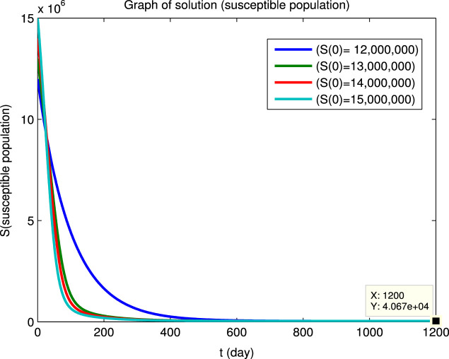
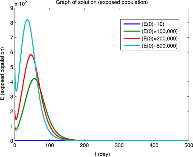
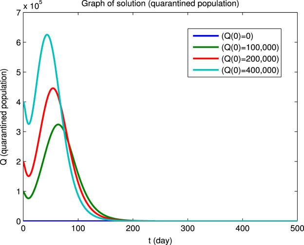
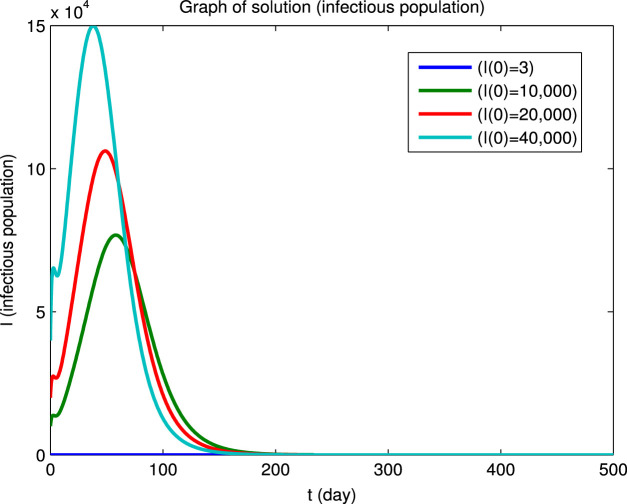
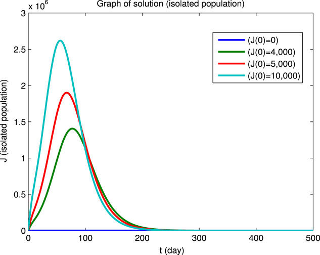
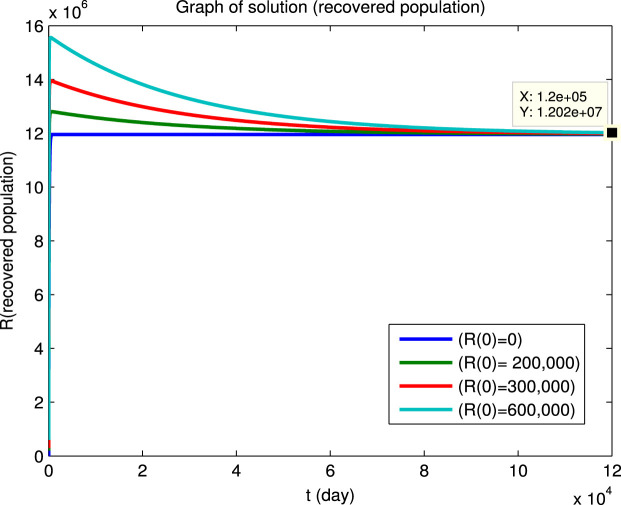
Using the Matlab program we have numerically integrated the system of Eqs. (40) for the four sets of initial conditions given in Table 5 to obtain the dynamical solutions shown in Fig. 2. The graphs show that, for the four different sets of initial conditions, the four infected populations first decrease and then increase before finally converging to zero, i.e., the initial points are not locally asymptotically stable even though there is long-term convergence to the disease-free equilibrium point. However, it can also be seen that at the longer times, where the population values are close to the disease-free equilibrium point, the solutions converge asymptotically to this equilibrium state. This behavior for the longer times in Fig. 2 is in agreement with Eq. (41) and the values of the reproduction numbers and eigenvalues given above.

Table 5.

Initial population values used for numerical integration.

Set	$S\left(0\right)$	$E\left(0\right)$	$Q\left(0\right)$	$I\left(0\right)$	$J\left(0\right)$	$R\left(0\right)$
1	$12\times 10^6$	10	0	3	0	0
2	$13\times 10^6$	$1\times 10^5$	$1\times 10^5$	$1\times 10^4$	$4\times 10^3$	$2\times 10^5$
3	$14\times 10^6$	$2\times 10^5$	$2\times 10^5$	$2\times 10^4$	$5\times 10^3$	$3\times 10^5$
4	$15\times 10^6$	$5\times 10^5$	$4\times 10^5$	$4\times 10^4$	$1\times 10^4$	$6\times 10^5$

Fig. 2.

Example of convergence to a disease-free equilibrium for four different sets of initial conditions. The $E$, $Q$, $I$, $J$ populations rapidly converge to zero and the $S$ and $R$ populations converge to equilibrium values $S_1^{\ast }=40661$ and $R_1^{\ast }=1.196\times 10^7$ (Beijing).

Fig. 2(a).

(a) Susceptible population.

Fig. 2(b).

(b) Exposed population.

Fig. 2(c).

(c) Quarantined population.

Fig. 2(d).

(d) Infectious population.

Fig. 2(e).

(e) Isolated population.

Fig. 2(f).

(f) Recovered population.

7.3. Sensitivity analysis of disease-free reproduction number

Using the analytical results given in Table 2, we have computed the normalized sensitivity indices shown in Table 6 of the disease-free reproduction number $R_{df}=0.01366<1$ for the parameter values of Table 4 and $\nu =0.01$. For these parameter values, the sensitivity indices $\Phi \left(R_{df}\right|\beta )$, $\Phi \left(R_{df}\right|{\epsilon }_E)$, $\Phi \left(R_{df}\right|{\epsilon }_Q)$, $\Phi \left(R_{df}\right|{\epsilon }_J)$, $\Phi \left(R_{df}\right|\mu )$, $\Phi \left(R_{df}\right|k_1)$ and $\Phi \left(R_{df}\right|k_2)$ are positive and the remaining indices are negative.

For these parameter values, $R_{df}=0.01366<1$ and the solution converges to a disease-free equilibrium point. Then, a reduction in the value of $R_{df}$ corresponds to a faster approach to equilibrium, i.e., to a faster disappearance of the disease. The values in column 2 of Table 6 are the sensitivity indices and the values in column 3 are % changes in parameter values required to give a $1\text{\%}$ decrease in $R_{df}$. For example, in order to get a $1\text{\%}$ decrease in the value of $R_{df}$, it is necessary to decrease the values of $\beta$, $\mu$, ${\epsilon }_J$, $k_1$ and $k_2$ by $1.000\text{\%}$, $1.004\text{\%}$, $1.055\text{\%}$, $198.8\text{\%}$ and $7428\text{\%}$, respectively. Also, in order to get a $1\text{\%}$ decrease in the value of $R_{df}$, it is necessary to increase the values of $\nu$, ${\sigma }_2$, $d_2$, ${\sigma }_1$, ${\gamma }_2$, $d_1$ and ${\gamma }_1$ by $1.003\text{\%}$, $1.156\text{\%}$, $12.2\text{\%}$, $26.2\text{\%}$, $112.2\text{\%}$, $196.9\text{\%}$ and $205.8\text{\%}$, respectively. Since the natural death rate $\mu$ cannot be easily changed, the most effective methods of reducing $R_{df}$ are to reduce the value of the infectiousness and contact rate $\beta$, increase the value of the immunization rate $\nu$, reduce the value of the isolation modification parameter ${\epsilon }_J$ and increase the value of the isolation recovery rate ${\sigma }_2$.

Table 6.

Normalized sensitivity indices $\Phi \left(R_{df}\right|h)$ and required % changes in parameter for 1% reduction in $R_{df}$ for disease-free equilibrium state (Beijing).

Param	$\Phi \left(R_{df}\right|h)$	% change	Param	$\Phi \left(R_{df}\right|h)$	% change
$\mu$	$+0.996$	$-1.004\text{\%}$	$\nu$	$-0.997$	$+1.003\text{\%}$
$\beta$	$+1.000$	$-1.000\text{\%}$	${\epsilon }_E$	$+0.000$	$+0.000\text{\%}$
${\epsilon }_Q$	$+0.000$	$+0.000\text{\%}$	${\epsilon }_J$	$+0.948$	$-1.055\text{\%}$
${\gamma }_1$	$-0.0049$	$+205.8\text{\%}$	${\gamma }_2$	$-0.0089$	$+112.2\text{\%}$
${\sigma }_1$	$-0.038$	$+26.2\text{\%}$	${\sigma }_2$	$-0.865$	$+1.156\text{\%}$
$k_1$	$+0.0050$	$-198.9\text{\%}$	$k_2$	$+0.0001$	$-7428\text{\%}$
$d_1$	$-0.0051$	$+196.9\text{\%}$	$d_2$	$-0.082$	$+12.2\text{\%}$

7.4. Endemic equilibrium point and asymptotic stability

For the Beijing parameter values in Table 4 and $\nu =0.000002$, we obtain the endemic equilibrium point

$$(S_2^{\ast },E_2^{\ast },Q_2^{\ast },I_2^{\ast },J_2^{\ast },R_2^{\ast },N_2^{\ast })=(2.78\times 10^6,1539.51,1231.277,281.532,6238.638,8.414\times 10^6,1.12\times 10^7).$$

The value of the disease-free reproduction number is $R_{df}=3.807>1$ and the value of the endemic reproduction number is $R_{en}=0.3756<1$. Further, the eigenvalues of the Jacobian for the disease-free equilibrium and for the endemic equilibrium are:

Disease-free

$$\begin{array}{ccc}{\lambda }_1=-0.000034\hfill & {\lambda }_2=-0.000036\hfill & {\lambda }_3=0.06618\hfill \\ {\lambda }_4=-0.5585\hfill & {\lambda }_5=-0.02134-0.059345i\hfill & {\lambda }_6=-0.02134+0.05935i.\hfill \end{array}$$

Endemic

$$\begin{array}{ccc}{\lambda }_1=-0.000034,\hfill & {\lambda }_2=-0.000062+0.00190i,\hfill & {\lambda }_3=-0.000062-0.00190i\hfill \\ {\lambda }_4=-0.5498,\hfill & {\lambda }_5=-0.1847+0.03302i,\hfill & {\lambda }_6=-0.1847-0.03302i.\hfill \end{array}$$

Therefore, the disease-free equilibrium point is unstable and the endemic equilibrium point is locally asymptotically stable.

As shown in Gumel et al. [6] (see also [9]), an endemic equilibrium point is also obtained for $\nu =0$.

7.5. Dynamical solutions for endemic equilibrium

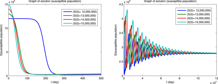
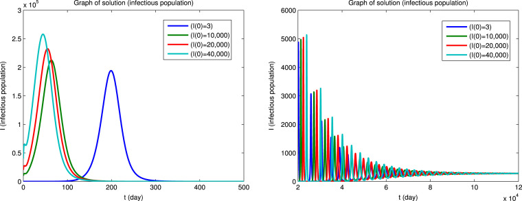
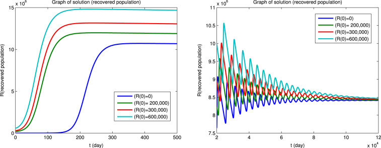
Using Matlab, we integrated the system of Eqs. (1), (2), (3), (4), (5), (6) for $\nu =0.000002$ for the four sets of initial conditions given in Table 5. Since the dynamical behavior for the four infected populations are similar, we will only show the solutions for the infectious population ($I$) and for the susceptible ($S$) and recovered ($R$) populations. The solutions for the $S$, $I$ and $R$ populations are shown in Fig. 3 first for a short integration time to show the initial behavior and then for a long integration time to show the convergence to an endemic equilibrium. It can be seen that the convergence to the endemic equilibrium is very slow and that many disease outbreaks occur during this period. This type of behavior was very common in “childhood” diseases such as measles, mumps, poliomyelitis, rubella, whooping cough etc. before vaccines became available for these diseases. Although it is difficult to see in Fig. 3, we found that epidemics can recur when the fraction of the susceptible population exceeds a certain critical level due to births or if the population of the immune recovered population falls below a certain critical level due to deaths. Similar results for the dynamical behavior of populations in the endemic region have also been reported by Koonprasert et al. [9] in a study on the effectiveness of quarantine and isolation in an SEQIJR model.

Fig. 3.

Example of convergence to an endemic equilibrium for four different sets of initial conditions (Beijing). The graphs in the left column show the initial behavior for $0\le t\le 500$ days. The graphs in the right column show the long-time behavior for $20000\le t\le 120000$ days.

Fig. 3(a).

(a) Susceptible population.

Fig. 3(b).

(b) Infectious population.

Fig. 3(c).

(c) Recovered population.

7.6. Sensitivity analysis of the endemic equilibrium point

In the sensitivity analysis we do not consider variations in $\Pi$, $\mu$, ${\epsilon }_E$ and ${\epsilon }_Q$. The parameter $\Pi$ represents the natural birth rate and the parameter $\mu$ represents the natural death rate for the population. These parameters cannot be changed easily for human populations. Also, we omit the modification parameters for infection from the exposed population ${\epsilon }_E$ and the quarantined population ${\epsilon }_Q$ since these parameters have been assumed to be zero. We therefore only consider sensitivity indices for the remaining eleven parameters.

Using the analytical results given in Table 3 and Eq. (36), and the parameter values in Table 4 with $\nu =0.000002$, we obtain the values shown in Table 7 for the normalized sensitivity indices of the endemic equilibrium populations. As noted above, the values of $R_{df}=3.807>1$ and $R_{en}=0.3756<1$ show that the endemic equilibrium is locally asymptotically stable. Since the sensitivity indices are functions of parameter values, the values in Table 7 will change if parameter values are changed. The interpretation of these indices is that a positive index means that $I_2^{\ast }$ increases if the parameter value is increased and a negative index means that $I_2^{\ast }$ decreases if the parameter value is increased with the magnitude giving the rate of change.

Table 7.

Sensitivity indices for endemic equilibrium state (Beijing).

Parameter	Sensitivity indices
	$S_2^{\ast }$	$E_2^{\ast }$	$Q_2^{\ast }$	$I_2^{\ast }$	$J_2^{\ast }$	$R_2^{\ast }$	$N_2^{\ast }$
$\beta$	−1.0237	+0.3326	+0.3326	+0.3326	+0.3326	+0.3062	−0.0237
${\epsilon }_J$	−0.9703	+0.3152	+0.3152	+0.3152	+0.3152	+0.2902	−0.0225
$\nu$	+0.0013	−0.0185	−0.0185	−0.0185	−0.0185	+0.0013	+0.0013
${\gamma }_1$	+0.0055	−0.5017	+0.4983	−0.5017	+0.0206	−0.0009	+0.0006
${\gamma }_2$	+0.0101	−0.0033	−0.0033	−0.9176	+0.0376	−0.0017	+0.0012
$k_1$	−0.0057	−0.4981	−0.4981	+0.5019	−0.0204	+0.0012	−0.0007
$k_2$	−0.0002	+0.0001	−0.9997	+0.0001	+0.0002	+0.0002	−0.00001
${\sigma }_1$	+0.0418	−0.0136	−0.0136	−0.0891	−0.0497	−0.0089	+0.0037
${\sigma }_2$	+0.9481	−0.3080	−0.3080	−0.3080	−1.2205	−0.2013	+0.0832
$d_1$	+0.0014	−0.0005	−0.0005	−0.0105	−0.0053	−0.0054	−0.0037
$d_2$	+0.0214	−0.0070	−0.0070	−0.0070	−0.0938	−0.0880	−0.0608

In order to reduce the spread of the disease, it is necessary to reduce the infectious population ($I_2^{\ast }$) and isolated population ($J_2^{\ast }$) since these populations are capable of direct transmission of the disease to uninfected people. It is also desirable to reduce the number of deaths from the disease, i.e., to increase the total surviving population $N_2^{\ast }$.

From the indices in Table 7, the most effective methods of reducing $I_2^{\ast }$ are, in order, to increase the isolation rate (${\gamma }_2$), reduce the transfer rate from exposed to infectious population ($k_1$), increase the quarantine rate (${\gamma }_1$) and reduce the contact rate between infectious and susceptible people ($\beta$). The most effective methods of reducing $J_2^{\ast }$ are, in order, to increase the recovery rate of isolated individuals (${\sigma }_2$), reduce the contact rate $\beta$, and reduce the modification parameter ${\epsilon }_J$. It can be seen from Table 7 that increasing the death rates $d_1$ and $d_2$ of the infectious and isolated individuals would also reduce the infectious and isolated populations. This method is clearly not an acceptable control method for a human disease. However, this method was adopted as an effective control method in the case of the spread of avian flu among chickens in China and “mad-cow disease” in England, and it has also been used as an effective method of controlling some other diseases among animals and plants.

The most effective methods for increasing the total surviving population $N_2^{\ast }$, i.e., to reduce the death rate, are, in order, increase the recovery rate of infectious individuals (${\sigma }_2$), reduce the contact rate $\beta$ and reduce the modification parameter ${\epsilon }_J$, i.e., to reduce the level of nosocomial disease as discussed in the introduction.

8. Comparison of results for Beijing, Canada, Hong Kong and Singapore

Using the parametervalues given in Table 4, we have computed and compared the disease-free and endemic results for the four regions. The overall behavior of the results for all four regions is similar, but with some differences in detail. We will compare the results for the reproduction numbers, the sensitivity indices and the critical immunity levels.

8.1. Reproduction numbers and sensitivity indices

The results for the basic reproduction numbers and the disease-free and endemic reproduction numbers are shown in Table 8. For each case, we have numerically integrated the differential equations and checked the asymptotic stability of equilibrium points by computing the value of the reproduction numbers and by computing the eigenvalues of the Jacobian matrices. In all cases we have shown that the numerical results agree with the theoretical analysis.

Table 8.

Reproduction numbers.

	Beijing	Canada	Hong Kong	Singapore
Disease-free	$\nu =0.01$
$R_0$	4.031	1.708	2.804	1.082
$R_{df}$	0.01366	0.005787	0.009502	0.003668
Endemic	$\nu =0.000002$
$R_{df}$	3.807	1.613	2.649	1.022
$R_{en}$	0.3756	0.6887	0.4863	0.9786

For each of the four regions, we have also computed the sensitivity indices of the disease-free reproduction number $R_{df}$ and the endemic equilibrium populations for all of the parameters in the model.

From these calculations, we can rank the indices in order of effectiveness in reducing a disease. The results for the disease-free equilibrium $R_{df}$ are shown in Table 9. The table shows the top three indices for each region for a disease-free case ($R_{df}<1$), and a critical immunization case $R_{df}\approx 1$.

Table 9.

Ranking for best parameters to reduce $R_{df}$.

Region	$R_{df}<1$	$R_{df}\approx 1$
Beijing	$\beta ,\nu ,\left(\mu \right),{\epsilon }_J$	$\beta ,{\epsilon }_J,{\sigma }_2$
Canada	$\beta ,\nu ,\left(\mu \right),{\epsilon }_J$	$\beta ,{\epsilon }_J,{\sigma }_2$
Hong Kong	$\beta ,\nu ,\left(\mu \right),{\epsilon }_J$	$\beta ,{\epsilon }_J,{\sigma }_2$
Singapore	$\beta ,\nu ,\left(\mu \right),{\epsilon }_J$	$\beta ,{\epsilon }_J,{\sigma }_2$

For $R_{df}<1$, the rankings for all regions are the same. The most effective methods of reducing $R_{df}$ are, in order, to reduce the infectiousness and contact rate $\beta$ between infectious and susceptible people, increase the value of the immunization rate $\nu$ and reduce the modification parameter ${\epsilon }_J$ for the infectiousness and contact rate of isolated people. It can be seen from Table 9 that reducing (index is positive) the natural death rate $\mu$ is the third most effective method of reducing the value of $R_{df}$. However, since the natural death rate cannot be varied easily for human populations, this is not an acceptable control method for a human disease. For $R_{df}\approx 1$, the most effective methods of reducing $R_{df}$ are, in order, to reduce the infectiousness and contact rate $\beta$, reduce the isolation modification parameter ${\epsilon }_J$ and increase the recovery rate of isolated individuals ${\sigma }_2$.

Table 10 shows the rankings for the most effective methods for reducing the endemic infectious populations $I_2^{\ast }$ in the four regions for $R_{df}\approx 1$ and for $R_{df}>1$. For $R_{df}\approx 1$, the rankings for Beijing, Canada, Hong Kong are the same. The most effective methods of reducing $I_2^{\ast }$ are, in order, to reduce the contact and infectiousness rate $\beta$, increase the recovery rate of isolated individuals ${\sigma }_2$ and increase the value of the immunization rate $\nu$. For Singapore, the most effective methods of reducing $I_2^{\ast }$ are, in order, to reduce the infectiousness and contact rate $\beta$, increase the recovery rate of isolated individuals ${\sigma }_2$ and increase the isolation rate ${\gamma }_2$.

Table 10.

Ranking for best parameters to reduce $I_2^{\ast }$.

Region	$R_{df}\approx 1$	$\nu$ value for $R_{df}\approx 1$	$R_{df}>1$	$\nu$ value for $R_{df}>1$
Beijing	$\beta ,{\sigma }_2,\nu$	0.0001	${\gamma }_2,k_1,{\gamma }_1$	0.000002
Canada	$\beta ,{\sigma }_2,\nu$	0.000024	$\beta ,{\sigma }_2,{\gamma }_2$	0.000002
Hong Kong	$\beta ,{\sigma }_2,\nu$	0.000061	${\gamma }_2,\beta ,k_1$	0.000002
Singapore	$\beta ,{\sigma }_2,{\gamma }_2$	0.0000028	$\beta ,{\sigma }_2,{\gamma }_2$	0.000002

For $R_{df}>1$, the most effective methods of reducing $I_2^{\ast }$ for Beijing are, in order, to increase the isolation rate ${\gamma }_2$, reduce the transfer rate from exposed to infectious $k_1$ and increase the quarantine rate ${\gamma }_1$. For Canada the most effective methods of reducing $I_2^{\ast }$ are, in order, to reduce the infectiousness and contact rate $\beta$, increase the recovery rate of isolated individuals ${\sigma }_2$ and increase the isolation rate ${\gamma }_2$. For Hong Kong the most effective methods of reducing $I_2^{\ast }$ are, in order, to increase the isolation rate ${\gamma }_2$, reduce the infectiousness and contact rate $\beta$ and reduce the transfer rate from exposed to infectious $k_1$. For Singapore the most effective methods of reducing $I_2^{\ast }$ are the same as for the $R_{df}\approx 1$ case.

8.2. Critical immunity levels

The critical values of the immunization rate $\nu$ and the critical ratio of recovered to total population can be calculated from Eqs. (38) and (39) and parameter values in Table 4 for the SARS epidemics in Beijing, Canada, Hong Kong and Singapore in 2002 and 2003. The results for the four regions are shown in Table 11. The results show that there is a big difference between the critical immunization levels and critical immunized ratio in the four regions. The difference is due to the different values of the basic reproduction number $R_0=\frac{{\alpha }_L}{{\alpha }_S}$ in the four regions. The difference in $R_0$ values in turn is mainly due to differences in the values of the infection factor $\beta$ and the modification factors for infection from the quarantined population (${\epsilon }_Q$) and the isolated population (${\epsilon }_J$).

Table 11.

Critical immunization levels for prevention of disease.

	Beijing	Canada	Hong Kong	Singapore
Critical $\nu$	$1.03\times 10^{-4}$	$2.407\times 10^{-5}$	$6.135\times 10^{-5}$	$2.803\times 10^{-6}$
Critical R/N ratio	0.7519	0.4415	0.6434	0.07616

9. Discussion and conclusions

We have studied an SEQIJR model for infectious disease transmission which generalizes the model developed by Gumel et al. [6] for the SARS epidemics of 2002 and 2003 by including immunization and a varying total populations size.

We have shown analytically that this model has a disease-free equilibrium state which always exists and an endemic equilibrium state which exists if and only if the disease-free equilibrium is unstable. We have defined generalized reproduction numbers $R_g$ for any given equilibrium state such that the state is locally asymptotically stable if $R_g<1$ and unstable if $R_g>1$. As special cases, we have obtained simple formulas for the reproduction numbers for a 100% susceptible population (the basic reproduction number $R_0=\frac{{\alpha }_L}{{\alpha }_S}$) and for the disease-free equilibrium $R_{df}=\frac{\mu {\alpha }_L}{(\mu +\nu ){\alpha }_S}$ by both the next-generation method [23] and from the eigenvalues of the Jacobian of the linearized model about the disease-free equilibrium. In these formulas, ${\alpha }_L$ can be interpreted as the rate of new infections from all infected individuals and ${\alpha }_S$ as the rate of reduction of the susceptible population due to transfers to other population groups including to the recovered immune group. The effect of the immunization rate ($\nu$) in reducing the reproduction number and increasing the stability of disease-free equilibrium states can be clearly seen by comparing the $R_0$ and $R_{df}$ formulas. We have also obtained simple formulas for a reproduction number $R_{en}$ for the endemic equilibrium state and shown that the endemic equilibrium is locally asymptotically stable if $R_{en}<1$ and does not exist if $R_{en}>1$.

We have also derived formulas for sensitivity indices of the disease-free and basic reproduction numbers, and the endemic equilibrium populations for changes in the values of model parameters.

For the numerical study of the model, we have used values of model parameters estimated by Gumel et al. [6] for the SARS epidemics in 2002–2003 in Beijing, Canada, Hong Kong and Singapore. For each of the four regions we have considered parameter values corresponding to a disease-free equilibrium and an endemic equilibrium. From the computed sensitivity indices for each of the regions, we have shown that the most important parameters for reducing infection are, in order, (1) for high immunization rates ($\nu \approx 0.01$) reduce the overall infection rate ($\beta$), increase the immunization rate, and reduce the modification factor for infection by isolated individuals (${\epsilon }_J$), (2) for critical immunization rates with $R_{df}\approx 1$, reduce $\beta$, reduce ${\epsilon }_J$ and increase recovery rate of isolated individuals (${\sigma }_2$), (3) for low immunization rates (endemic equilibrium) the most important for Beijing and Hong Kong is to increase the isolation rate of infectious individuals (${\gamma }_2$) and the most important for Canada and Singapore is to reduce $\beta$.

The numerical results for the reproduction numbers and the sensitivity indices clearly support the importance of isolation and to a lesser extent quarantine in controlling the spread of a disease.

We have obtained very simple formulas in terms of the basic reproduction number $R_0$ for critical values of the immunization rate and the ratio of the recovered (immune) and total populations that are required to stop the spread of a disease. Our numerical results for the four regions considered in this paper clearly support the importance that is now widely accepted, except by anti-vax campaigners, of maintaining a critical immunization level of “herd immunity” to stop the spread of a disease. The differences in the critical values of the immunization rate in the four regions clearly show the importance of factors such as reducing infection rates, and increasing isolation and quarantine, in stopping an epidemic that can occur when the immunization ratio falls below a critical level.

Unfortunately, in 2002 and 2003 there was no known immunization available for SARS. Therefore, the immunization results in this paper are not relevant for the SARS outbreaks of 2002–2003. However, the inclusion of immunization in the study of an SEQIJR model is important as the SEQIJR model is a very general model which can be applied to a number of other diseases that are also mainly transmitted by person to person contact and for which immunization is available, e.g., influenza and “childhood diseases” such as measles, mumps, whooping cough etc. A similar model with the addition of a bird reservoir of the disease could also be used to analyze avian influenza. SEIR models have, of course, been studied by many authors and there is now an extensive literature on them. However, we would note that the formulas for generalized reproduction numbers, sensitivity indices and critical immunization levels for the SEQIJR model could easily be applied to SEIR models by removing the quarantined and isolated compartments and suitably redefining some of the parameters.

References

- 1.Brauer F., Castillo-Chávez C. Mathematical Models in Population Biology and Epidemiology. Springer-Verlag; New York: 2001. [Google Scholar]
- 2.Chitnis N., Hyman J.M., Cushing J.M. Determining important parameters in the spread of malaria through the sensitivity analysis of a mathematical model. Bull. Math. Biol. 2008;70:1272–1296. doi: 10.1007/s11538-008-9299-0. [DOI] [PubMed] [Google Scholar]
- 3.Chowell G., Fenimore P.W., Castillo-Garsow M.A., Castillo-Chavez C. SARS outbreaks in Ontario,Hong Kong and Singapore: the role of diagnosis and isolation as a control mechanism. J. Theoret. Biol. 2003;224:1–8. doi: 10.1016/S0022-5193(03)00228-5. [DOI] [PMC free article] [PubMed] [Google Scholar]
- 4.Diamond B. SARS spreads new outlook on quarantine models. Nat. Med. 2003;9:1441. doi: 10.1038/nm1203-1441a. [DOI] [PMC free article] [PubMed] [Google Scholar]
- 5.Getz W.M., Lloyd-Smith J.O., Cross P.C., Bar-David S., Johnson P.L., Porco T.C., Sánchez M.S. Modeling the Invasion and Spread of Contagious Diseases in Heterogeneous Populations. 2005. pp. 1–32. (DIMACS Series in Discrete Mathematics and Theoretical Computer Science). [Google Scholar]
- 6.Gumel A.B., Ruan S., Day T., Watmough J., Brauer F., van den Driessche P., Gabrielson D., Bowman C., Alexander M.E., Ardal S., Wu J., Sahai B.M. Modelling strategies for controlling SARS outbreaks. Proc. R. Soc. Lond. Ser. B. 2004;271:2223–2232. doi: 10.1098/rspb.2004.2800. [DOI] [PMC free article] [PubMed] [Google Scholar]
- 7.Hsieh Y.H., Chen C.W.S., Hsu S.B. SARS outbreak, Taiwan, 2003. Emerg. Infect. Diseases. 2004;10:201–206. doi: 10.3201/eid1002.030515. [DOI] [PMC free article] [PubMed] [Google Scholar]
- 8.Janreung S. Using a Mathematical Model to Study the Effect of Quarantine and Isolation for Controlling SARS Outbreaks. King Mongkut’s University of Technology North Bangkok; 2008. (M.Sc.(Appl. Math.) thesis) [Google Scholar]
- 9.Koonprasert S., Janreung S., Moore E.J. An analysis of quarantine and isolation in an SEQIJR model. Far East J. Math. Sci. (FJMS) 2013:153–172. Special Volume 2013, Part II. [Google Scholar]
- 10.Kuznetsov Y.A. Elements of Applied Bifurcation Theory. Springer; New York, NY, USA: 1998. [Google Scholar]
- 11.Lee N., Hui D., Wu A., Chan P., Cameron P., Joynt G.M., Ahuja A., Yung M.Y., Leung C.B., To K.F., Lui S.F., Szeto C.C., Chung S., Sung J.J. A major outbreak of severe acute respiratory syndrome in Hong Kong. N. Engl. J. Med. 2003;348:1986–1994. doi: 10.1056/NEJMoa030685. [DOI] [PubMed] [Google Scholar]
- 12.Li M.Y., Graef J.R., Wang L., Karsai J. Global dynamics of a SEIR model with varying total population size. Math. Biosci. 1999;160:191–213. doi: 10.1016/s0025-5564(99)00030-9. [DOI] [PubMed] [Google Scholar]
- 13.Lipsitch M., Cohen T., Cooper B., Robins J.M., Ma S., James L., Gopalakrishna G., Chew S.K., Tan C.C., Samore M.H., Fisman D., Murray M. Transmission dynamics and control of severe acute respiratory syndrome. Science. 2003;300:1966–1970. doi: 10.1126/science.1086616. [DOI] [PMC free article] [PubMed] [Google Scholar]
- 14.Z. Liu, K. He, L. Yang, C. Bian, Z. Wang, Characterizing transmission and control of the SARS epidemic: Novel stochastic spatio-temporal models, in: Conf. Proc. IEEE, Engineering in Medicine and Biology, 2005, pp. 7463–7469. [DOI] [PubMed]
- 15.Lloyd-Smith J.O., Galvani A.P., Getz W.M. Curtailing transmission of severe acute respiratory syndrome within a community and its hospital. Proc. R. Soc. Lond. 2003;B270:1979–1989. doi: 10.1098/rspb.2003.2481. [DOI] [PMC free article] [PubMed] [Google Scholar]
- 16.Luenberger D.G. Introduction to Dynamic Systems: Theory, Models and Applications. John Wiley and Sons; New York: 1979. [Google Scholar]
- 17.MedicineNet.com. Available from: URL: http://www.medicinenet.com/severe_acute_respiratory_syndrome_sars/article.htm (Last viewed: 03.06.16).
- 18.Minnesota Department of Health. Available from: URL: http://www.health.state.mn.us/divs/idepc/diseases/sars/basics.html (Last viewed: 03.06.16).
- 19.Ou J., Li Q., Zeng G. Efficiency of quarantine during an epidemic of severe acute respiratory syndrome-Beijing. China. MMWR. 2003;52:1037–1040. [PubMed] [Google Scholar]
- 20.Pang X.I., Zhu Z., Xu F., Guo J., Gong X., Liu D., Liu Z., Chin D.P., Feikin D.R. Evaluation of control measures implemented in the severe acute respiratory syndrome outbreak in Beijing, 2003. JAMA. 2003;290:3215–3221. doi: 10.1001/jama.290.24.3215. [DOI] [PubMed] [Google Scholar]
- 21.Riley S., Fraser C., Donnelly C.A., Ghani A.C., Abu-Raddad L.J., Hedley A.J., Leung G.M., Ho L.-M., Lam T.-H., Thach T.Q., Chau P., Chan K.-P., Lo S.-V., Leung P.-Y., Tsang T., Ho W., Lee K.-H., Lau E.M.C., Ferguson N.M., Anderson R.M. Transmission dynamics of etiological agent of SARS in Hong Kong: the impact of public health interventions. Science. 2003;300:1961–1966. doi: 10.1126/science.1086478. [DOI] [PubMed] [Google Scholar]
- 22.Samsuzzoha Md., Singh M., Lucy D. Uncertainty and sensitivity analysis of the basic reproduction number of a vaccinated epidemic model of influenza. Appl. Math. Model. 2013;37:903–915. [Google Scholar]
- 23.van den Driessche P., Watmough J. Reproduction numbers and sub-threshold endemic equilibria for compartmental models of disease transmission. Math. Biosci. 2002;180:29–48. doi: 10.1016/s0025-5564(02)00108-6. [DOI] [PubMed] [Google Scholar]
- 24.Wai T., Turinici G., Danchin A. A double epidemic model for the SARS propagation. BMC Infect. Dis. 2003;3:19. doi: 10.1186/1471-2334-3-19. [DOI] [PMC free article] [PubMed] [Google Scholar]
- 25.Wang Y., Liu J., Liu L. Viral dynamics of an HIV model with latent infection incorporating antiretroviral therapy. Adv. Differential Equations. 2016;2016:225–240. [Google Scholar]
- 26.Wang W., Ruan W.S. Simulating the SARS outbreak in Beijing with limited data. J. Theoret. Biol. 2004;227:369–379. doi: 10.1016/j.jtbi.2003.11.014. [DOI] [PMC free article] [PubMed] [Google Scholar]
- 27.Wang X., Wei L., Zhang J. Dynamical analysis and perturbation solution of an SEIR epidemic model. Appl. Math. Comput. 2014;232:479–486. [Google Scholar]
- 28.Webb G.F. Critical role of nosocomial transmission in the toronto SARS outbreak. Math. Biosci. Eng. 2004;1:1–13. doi: 10.3934/mbe.2004.1.1. [DOI] [PubMed] [Google Scholar]
- 29.Yi N., Zhang Q., Mao K., Yang D., Li Q. Analysis and control of an SEIR epidemic system with nonlinear transmission rate. Math. Comput. Modelling. 2009;50:1498–1513. doi: 10.1016/j.mcm.2009.07.014. [DOI] [PMC free article] [PubMed] [Google Scholar]
- 30.Zhou Y., Ma Z., Brauer F. A discrete epidemic model for SARS transmission and control in China. Math. Comput. Modelling. 2004;40:1491–1506. doi: 10.1016/j.mcm.2005.01.007. [DOI] [PMC free article] [PubMed] [Google Scholar]