Bifurcations of an epidemic model with non-monotonic incidence rate of saturated mass action

Abstract

In this paper, we study the bifurcations of an epidemic model with non-monotonic incidence rate of saturated mass action, which describes the psychological effects of the community on certain serious diseases when the number of infective is getting larger. By carrying out the bifurcation analysis of the model, we show that there exist some values of the model parameters such that numerous kinds of bifurcation occur for the model, such as Hopf bifurcation, Bogdanov–Takens bifurcation.

1. Introduction

In the mathematical modeling of disease transmission, there is a classic model proposed by Kermack and McKendrick [8] in 1927. They divided the population being studied in time t into three classes labeled S(t), I(t) and R(t), where S(t) is the number of susceptible individuals, I(t) is the number of infective individuals, and R(t) is the number of removed individuals at time t, respectively. And they assumed that a rate of contacts by an infective with a susceptible is proportional to population size with constant of proportionality. It is clear that the assumption is too simple. Later Capasso and Serio [2] introduced a saturated incidence rate g(I)S into the epidemic model after studying the cholera epidemic spread in Bari in 1973, which describes the contact between infective individuals and susceptible individuals, where

$$g(I)=\frac{\mathit{kI}}{1+\alpha I}\text{,}$$

kI measures the infection force of the disease and 1/(1 +  αI) measures the inhibition effect from the behavioral change of the susceptible individuals when their number increases. g(I) tends to a saturation level when I gets large.

The general incidence rate

$$\frac{{\mathit{kI}}^{p}S}{1+\alpha I^q}$$

was proposed by Liu et al. [13], [14] and used by a number of authors, see, for example, [3], [5], [7], [1], etc. For a specific nonlinear incident rate

$$\frac{{\mathit{kI}}^{2}S}{1+\alpha I^2}\text{,}$$

Ruan and Wang in [16] studied an epidemic model with this specific nonlinear incident rate and obtained lots of interesting dynamical behaviors of the model such as a limit cycle, two limit cycles and homoclinic loop, etc. Note that these functions g(I) of the incident rate g(I)S is monotone, which means that the contact rate between infective individuals and susceptible individuals is bigger and bigger as the number of infective individuals is getting larger. However, it is not true in reality. For example, in the recent outbreak of epidemic of severe acute respiratory syndrome (SARS) the “psychological” effects on the general public (see [4], [9]), aggressive measures and policies, such as border screening, mask wearing, quarantine, isolation, etc. may tend to reduce the number of contacts per unit time as the number of infective’s were getting relatively larger. To model this phenomenon, Xiao and Ruan in [18] considered a special nonlinear incident rate

$$\frac{\mathit{kIS}}{1+\alpha I^2}\text{,}$$

where g(I) is non-monotone. When I is small, g(I) is increasing. Because of small number of infective’s, people may ignore the epidemic, which may lead to lots of effective contacts between the infective individuals and suspectable. And when I is getting larger and larger, g(I) is decreasing since many protection measures could be taken by the susceptible individuals. In [18], Xiao and Ruan presented the global analysis of an epidemic model with the non-monotonic incident rate and obtained either the number of infective individuals tends to zero as time evolves or the disease persists. Hence, the model cannot undergo any bifurcations.

In this paper we consider a general non-monotonic incidence rate

$$\frac{\mathit{kIS}}{1+\beta I+\alpha I^2}$$

in an epidemic model, which is described by the following form:

$$\begin{array}{cc}\hfill & \frac{\mathrm{d}S}{\mathrm{d}t}=b-\mathit{dS}-\frac{\mathit{kSI}}{1+\beta I+\alpha I^2}+\delta R\text{,}\hfill \\ \hfill & \frac{\mathrm{d}I}{\mathrm{d}t}=\frac{\mathit{kSI}}{1+\beta I+\alpha I^2}-(d+\mu )I\text{,}\hfill \\ \hfill & \frac{\mathrm{d}R}{\mathrm{d}t}=\mu I-(d+\delta )R\text{,}\hfill \end{array}$$ (1.1)

where S(t), I(t) and R(t) denote the numbers of susceptible, infective, and recovered individuals at time t, respectively, b is the recruitment rate of the population, d is the natural death rate of the population, k is the proportionality constant, μ is the natural recovery rate of the infective individuals, δ is the rate at which recovered individuals lose immunity and return to the susceptible class, α is a positive parameter, β is a parameter such that 1 +  βI  +  αI ²  > 0 for all I  ⩾ 0, hence, $\beta >-2\sqrt{\alpha }$.

From the standpoint of biology, we are interested only in the dynamics of system (1.1) in the first octant of ${\mathbb{R}}^3$. Before going to details of dynamics for (1.1), we first present the following lemma which is easily proved.

Lemma 1.1

The plane S   +   I   +   R   =   b/d is an invariant manifold of system (1.1) , which is attracting in the first octant of ${\mathbb{R}}^3$ .

This lemma implies that the limit set of system (1.1) in the first octant of ${\mathbb{R}}^3$ locates on the plane S  +  I  +  R  =  b/d. Therefore, the dynamics of system (1.1) in the first octant of ${\mathbb{R}}^3$ is equivalent to the following system:

$$\begin{array}{cc}\hfill & \frac{\mathrm{d}I}{\mathrm{d}t}=\frac{\mathit{kI}}{1+\beta I+\alpha I^2}\left(\frac{b}{d}-I-R\right)-(d+\mu )I\text{,}\hfill \\ \hfill & \frac{\mathrm{d}R}{\mathrm{d}t}=\mu I-(d+\delta )R\hfill \end{array}$$ (1.2)

in the first quadrant ${\mathbb{R}}_{+}^2$ of ${\mathbb{R}}^2$. System (1.1) has the disease-free equilibrium and the endemic equilibria if and only if system (1.2) has the equilibrium (0, 0) and the positive equilibria, respectively. It is clear that system (1.1) always has a disease-free equilibrium E ₀  = (b/d, 0, 0) for all values of parameters. To find the endemic equilibria, we investigate the existence of the positive equilibria of system (1.2). For simplicity, we re-scale (1.2) by

$$x=\frac{k}{d+\delta }I\text{,}y=\frac{k}{d+\delta }R\text{,}\tau =(d+\delta )t\text{.}$$

Then we obtain

$$\begin{array}{cc}\hfill & \frac{\mathrm{d}x}{\mathrm{d}\tau }=\frac{x}{1+\mathit{mx}+{\mathit{nx}}^2}(A-x-y)-\mathit{px}\text{,}\hfill \\ \hfill & \frac{\mathrm{d}y}{\mathrm{d}\tau }=\mathit{qx}-y\text{,}\hfill \end{array}$$ (1.3)

where

$$m=\frac{\beta (d+\delta )}{k}\text{,}n=\frac{\alpha (d+\delta {)}^2}{k^2}\text{,}A=\frac{\mathit{bk}}{d(d+\delta )}\text{,}p=\frac{d+\mu }{d+\delta }\text{,}q=\frac{\mu }{d+\delta }\text{.}$$

It can been seen that A, p, q, n are positive parameters, $m>\frac{-2\sqrt{\alpha }(d+\delta )}{k}=-2\sqrt{n}$.

In this paper, we focus on studying the existence of non-hyperbolic positive equilibria of (1.3) and their bifurcations. To find the positive equilibria of system (1.3), we set

$$\begin{array}{cc}\hfill & \frac{x}{1+\mathit{mx}+{\mathit{nx}}^2}(A-x-y)-\mathit{px}=0\text{,}\hfill \\ \hfill & \mathit{qx}-y=0\text{,}\hfill \end{array}$$

which yields

$${\mathit{pnx}}^2+(1+q+\mathit{pm})x+p-A=0\text{.}$$ (1.4)

Note that

$$p-A=\frac{d^2+d\mu -\mathit{bk}}{d(d+\delta )}=\frac{(d-d_1)(d-d_2)}{d(d+\delta )}\text{,}$$

where $d_1=\frac{-\mu +\sqrt{{\mu }^2+4\mathit{bk}}}{2}>0$, $d_2=\frac{-\mu -\sqrt{{\mu }^2+4\mathit{bk}}}{2}<0$.

Setting R ₀  =  d ₁/d, we have p  −  A  ⩾ 0 if and only if R ₀  ⩽ 1. Let

$$\Delta =(1+q+\mathit{pm}{)}^2-4\mathit{pn}(p-A)\text{.}$$

Then we obtain the following lemma.

Lemma 1.2

• (i)
  System (1.3) has a unique positive equilibrium E ^∗ (x ^∗ ,   y ^∗ ) if and only if one of the following conditions holds:

  • (i.1)
    R ₀  >  1; in this case, $x^{\ast }=\frac{-(1+q+\mathit{pm})+\sqrt{(1+q+\mathit{pm}{)}^2-4\mathit{pn}(p-A)}}{2\mathit{pn}}$ , y ^∗   =   qx ^∗ .
  • (i.2)
    R ₀   =   1 and 1   +   q   +   pm  <  0; in this case, $x^{\ast }=-\frac{1+q+\mathit{pm}}{\mathit{pn}}$ , y ^∗   =   qx ^∗ .
  • (i.3)
    Δ   =   0 and 1   +   q   +   pm  <  0; in this case, $x^{\ast }=-\frac{1+q+\mathit{pm}}{2\mathit{pn}}$ , y ^∗   =   qx ^∗ .
• (ii) System (1.3) has two positive equilibria E ₁ (x ₁ ,   y ₁ ) and E ₂ (x ₂ ,   y ₂ ) if and only if Δ  >  0, R ₀  <  1 and 1   +   q   +   pm  <  0. In this case, $x_1=\frac{-(1+q+\mathit{pm})-\sqrt{(1+q+\mathit{pm}{)}^2-4\mathit{pn}(p-A)}}{2\mathit{pn}}$ , y ₁   =   qx ₁ ; $x_2=\frac{-(1+q+\mathit{pm})+\sqrt{(1+q+\mathit{pm}{)}^2-4\mathit{pn}(p-A)}}{2\mathit{pn}}$ , y ₂   =   qx ₂ .

The Jacobian matrix of system (1.3) at equilibrium (x,  y) is

$$M_1=\left[\begin{array}{cc}\hfill \frac{x({\mathit{nx}}^2+2{\mathit{nqx}}^2+{\mathit{mqx}}^2-2\mathit{nAx}-\mathit{Am}-1)}{(1+\mathit{mx}+{\mathit{nx}}^2{)}^2}\hfill & \hfill \frac{-x}{1+\mathit{mx}+{\mathit{nx}}^2}\hfill \\ \hfill q\hfill & \hfill -1\hfill \end{array}\right]\text{.}$$

Therefore, the determinant of the matrix M ₁ is

$$\det (M_1)=\frac{x(1+q+\mathit{Am}+2\mathit{nAx}-(1+q){\mathit{nx}}^2)}{(1+\mathit{mx}+{\mathit{nx}}^2{)}^2}\text{.}$$

Its sign is determined by

$$S_1\triangleq 1+q+\mathit{Am}+2\mathit{nAx}-(1+q){\mathit{nx}}^2\text{.}$$

And the trace of the matrix M ₁ is

$$\mathrm{tr}(M_1)=\frac{-n^2{x}^4+n(1+2q-2m)x^3+(\mathit{mq}-2\mathit{nA}-m^2-2n)x^2-(\mathit{Am}+2m+1)x-1}{(1+\mathit{mx}+{\mathit{nx}}^2{)}^2}\text{,}$$

the sign of which is determined by

$$S_2\triangleq -n^2{x}^4+n(1+2q-2m)x^3+(\mathit{mq}-2\mathit{nA}-m^2-2n)x^2-(\mathit{Am}+2m+1)x-1\text{.}$$

Note that pnx ²  + (1 +  q  +  pm)x  +  p  −  A  = 0. Then we have

$$\begin{array}{cc}\hfill & {\mathit{pS}}_1=[2\mathit{nAp}+(1+q)(1+q+\mathit{mp})]x+\mathit{Apm}+(1+q)(2p-A)\text{,}\hfill \\ \hfill & p^3{\mathit{nS}}_2=(B_{1}A+B_2)x+(B_{3}A+B_4)\text{,}\hfill \end{array}$$

where

$$\begin{array}{cc}\hfill & B_1=\mathit{np}(2+3p+2q+4\mathit{pq}+{\mathit{mp}}^2)\text{,}\hfill \\ \hfill & B_2=(1+q+\mathit{mp})[(1+q+\mathit{mp}{)}^2-2{\mathit{np}}^3+p(1+2q-2m)(1+q+\mathit{mp})+p^2(m^2-\mathit{mq})]+2{\mathit{mnp}}^4\text{,}\hfill \\ \hfill & B_3=-(1+q+\mathit{mp}{)}^2-p(1+q+\mathit{mp})(1+2q-2m)-p^2(m^2-\mathit{mq})+2{\mathit{np}}^3\text{,}\hfill \\ \hfill & B_4=p[(1+q+\mathit{mp}{)}^2+p(1+q+\mathit{mp})(1+2q-2m)-n(1+2p)A^2+p^2(m^2-\mathit{mq})]\text{.}\hfill \end{array}$$

From qualitative analysis, we obtain the following conclusion.

Theorem 1.3

• (i) The unique positive equilibrium E ^∗ (x ^∗ ,   y ^∗ ) of system (1.3) is a degenerate equilibrium if Δ   =   0 and 1   +   q   +   pm  <  0, where $x^{\ast }=-\frac{1+q+\mathit{pm}}{2\mathit{pn}}$ , y ^∗   =   qx ^∗ .
• (ii)
  The unique positive equilibrium E ^∗ (x ^∗ ,   y ^∗ ) of system (1.3) is a center-type equilibrium if R ₀  >  1, S ₂ (x ^∗ )   =   0, where

  $$x^{\ast }=\frac{-(1+q+\mathit{pm})+\sqrt{(1+q+\mathit{pm}{)}^2-4\mathit{pn}(p-A)}}{2\mathit{pn}}\text{,}{y}^{\ast }={\mathit{qx}}^{\ast }\text{.}$$
• (iii)
  System (1.3) has two positive equilibria E ₁ (x ₁ ,   y ₁ ) and E ₂ (x ₂ ,   y ₂ ) if Δ  >  0, R ₀  <  1 and 1   +   q   +   pm  <  0. And further when S ₂ (x ₂ )   =   0, E ₁ (x ₁ ,   y ₁ ) is a hyperbolic saddle, E ₂ (x ₂ ,   y ₂ ) is a center-type equilibrium, where

  $$\begin{array}{cc}\hfill & x_1=\frac{-(1+q+\mathit{pm})-\sqrt{(1+q+\mathit{pm}{)}^2-4\mathit{pn}(p-A)}}{2\mathit{pn}}\text{,}{y}_1={\mathit{qx}}_1\text{;}\hfill \\ \hfill & x_2=\frac{-(1+q+\mathit{pm})+\sqrt{(1+q+\mathit{pm}{)}^2-4\mathit{pn}(p-A)}}{2\mathit{pn}}\text{,}{y}_2={\mathit{qx}}_2\text{.}\hfill \end{array}$$

We will show that there exist some parameters values such that (1.3) has a cusp of codimension 3, and other parameters values such that (1.3) has a multiple focus. Choosing the original parameters of the model as bifurcation parameters, we discuss what bifurcations system (1.3) can undergo.

This paper is organized as follows. In Section 2, we show that there exist some values of parameters such that the model (1.3) has a unique positive equilibrium, which is a cusp of codimension 3. And there exists a set of values of parameters such that the model undergoes Bogdanov–Takens bifurcation of codimension 2 when two parameters vary in the small neighborhood of the set of parameter values. In Section 3, we show that there exist some values of parameters such that the model (1.3) has a positive equilibrium, which is a multiple focus of codimension 1 in two cases. Choosing one parameter of the model as a bifurcation parameter, we discuss the Hopf bifurcation of the model. The paper ends with a brief conclusion.

2. Bogdanov–Takens bifurcation

The purpose of this section is to study if there exist some values of model parameters such that model (1.3) undergoes the Bogdanov–Takens bifurcation. From Theorem 1.3, we know that the unique equilibrium E ^∗(x ^∗,  y ^∗) is degenerate if and only if (H1) Δ  = 0 and (H2) 1 +  q  +  pm  < 0. In order to guarantee the existence of Bogdanov–Takens bifurcation, we further assume that (H3) tr(M ₁(x ^∗)) = 0. Now we choose some values of parameters n, p, q, m and A such that (H1)–(H3) hold. We first show that there exists the value of model parameters such that E ^∗(x ^∗,  y ^∗) is a cusp of codimension 3. Taking m  = −7, p  = 2 and q  = 5, we obtain that n  = 20, A  = 8/5, x ^∗  = 1/10, y ^∗  = 1/2 by (H1)–(H3).

Lemma 2.1

When (m,   p,   q,   n,   A)   =   (−7,   2,   5,   20,   8/5), system (1.3) has a unique positive equilibrium (x ^∗ ,   y ^∗ )   =   (1/10,   1/2), which is a cusp of codimension 3.

Proof

Translating the unique positive equilibrium (1/10, 1/2) into the origin, we set X  =  x  − 1/10, Y  =  y  − 1/2, for simplicity, rewriting X, Y as x, y, respectively, then (1.3) becomes

$$\begin{array}{cc}\hfill & \frac{\mathrm{d}x}{\mathrm{d}\tau }=\frac{x+1/10}{1-7(x+1/10)+20(x+1/10{)}^2}(1-x-y)-2(x+1/10)\text{,}\hfill \\ \hfill & \frac{\mathrm{d}y}{\mathrm{d}\tau }=5x-y\text{.}\hfill \end{array}$$ (2.1)

Using Taylor expansion to (2.1), we obtain

$$\begin{array}{cc}\hfill & \frac{\mathrm{d}x}{\mathrm{d}\tau }=x-y/5-16\mathit{xy}/5+8x^2-56x^{2}y/5-72x^3+304x^{3}y/5-752x^4+\mathrm{O}((x\text{,}y{)}^5)\text{,}\hfill \\ \hfill & \frac{\mathrm{d}y}{\mathrm{d}\tau }=5x-y\text{.}\hfill \end{array}$$ (2.2)

Let X  =  x, Y  =  x  −  y/5, and rename X, Y as x, y. Then (2.2) is transformed into

$$\begin{array}{cc}\hfill & \frac{\mathrm{d}x}{\mathrm{d}\tau }=y-8x^2+16\mathit{xy}-128x^3+56x^{2}y-448x^4-304x^{3}y+\mathrm{O}((x\text{,}y{)}^5)\text{,}\hfill \\ \hfill & \frac{\mathrm{d}y}{\mathrm{d}\tau }=-8x^2+16\mathit{xy}-128x^3+56x^{2}y-448x^4-304x^{3}y+\mathrm{O}((x\text{,}y{)}^5)\text{.}\hfill \end{array}$$ (2.3)

In order to obtain the canonical normal forms, we set X  =  x  − 8x ²  + 200x ³/3 − 500x ⁴, Y  =  y  − 8x ², and rewriting X, Y as x, y, respectively. Then (2.3) becomes

$$\begin{array}{cc}\hfill & \frac{\mathrm{d}x}{\mathrm{d}\tau }=y\text{,}\hfill \\ \hfill & \frac{\mathrm{d}y}{\mathrm{d}\tau }=-8x^2-128x^3-200x^{2}y-4480x^4/3-3400x^{3}y+\mathrm{O}((x\text{,}y{)}^5)\text{,}\hfill \end{array}$$ (2.4)

From theorem in [19], the equilibrium (0, 0) of (2.4) is a cusp of codimension 3, which implies the conclusion. □

From Lemma 2.1, we can see when model parameters (m,  p,  q,  n,  A) vary in the small neighborhood of (−7, 2, 5, 20, 8/5), system (1.3) may undergo the cusp bifurcation of codimension 3 and some complicated dynamics will occur. However, this analysis of the cusp bifurcation of codimension 3 is too complicated to be done. We have to discuss if there exist model parameters such that system (1.3) can undergo the cusp bifurcation of codimension 2.

Taking m  = −4, p  = 2, q  = 3, from (H1) and (H3) we have A  = 5/3, n  = 6. In this case, system (1.3) has a unique positive equilibrium (1/6, 1/2). It is easy to check that the equilibrium is a cusp of codimension 2.

In the following we will find the universal unfolding of E(1/6, 1/2) by choosing parameters p and q as bifurcation parameters in a small neighborhood of (p,  A,  q,  m,  n) = (2, 5/3, 3, −4, 6). Let

$$p=2+{\lambda }_1\text{,}q=3+{\lambda }_2\text{.}$$

And rewriting τ as t, then (1.3) becomes

$$\begin{array}{cc}\hfill & \frac{\mathrm{d}x}{\mathrm{d}t}=\frac{x}{1-4x+6x^2}(5/3-x-y)-\mathit{px}\text{,}\hfill \\ \hfill & \frac{\mathrm{d}y}{\mathrm{d}t}=\mathit{qx}-y\text{,}\hfill \end{array}$$ (2.5)

where ∣λ ₁∣ ≪ 1 and ∣λ ₂∣ ≪ 1.

If λ ₁  = 0, λ ₂  = 0, then (1/6, 1/2) is a cusp of codimension 2 for (2.5). Let X  =  x  − 1/6, Y  =  y  − 1/2. By the Taylor expansion, we have (for simplicity, we still use x, y as X, Y, respectively)

$$\begin{array}{cc}\hfill & \frac{\mathrm{d}x}{\mathrm{d}t}=-{\lambda }_1/6+(1-{\lambda }_1)x-y/3+6x^2-10/3\mathit{xy}+w_1(x\text{,}y\text{,}\lambda )\text{,}\hfill \\ \hfill & \frac{\mathrm{d}y}{\mathrm{d}t}={\lambda }_2/6+(3+{\lambda }_2)x-y\text{,}\hfill \end{array}$$ (2.6)

where λ  = (λ ₁,  λ ₂), w ₁(x,  y,  λ) is a smooth function of x, y and λ at least of order three in x and y.

Set X  =  x, Y  = −λ ₁/6 + (1 + 2λ ₁/3)x  −  y/3, and rewriting X, Y as x, y, respectively, we get

$$\begin{array}{cc}\hfill & \frac{\mathrm{d}x}{\mathrm{d}t}=y+(-4-20{\lambda }_1/3)x^2+10\mathit{xy}+w_2(x\text{,}y\text{,}\lambda )\text{,}\hfill \\ \hfill & \frac{\mathrm{d}y}{\mathrm{d}t}=a_0+a_{1}x+2{\lambda }_{1}y/3+a_2{x}^2+a_3\mathit{xy}+w_3(x\text{,}y\text{,}\lambda )\text{,}\hfill \end{array}$$ (2.7)

where w ₂(x,  y,  λ), w ₃(x,  y,  λ) is a smooth function of x, y and λ at least of order three in x and y, and

$$a_0=-(3{\lambda }_1+{\lambda }_2)/18\text{,}{a}_1=(2{\lambda }_1-{\lambda }_2)/3\text{,}{a}_2=-4-28{\lambda }_1/3-40{\lambda }_1^2/9\text{,}{a}_3=10+20{\lambda }_1/3\text{.}$$

By setting X  =  x  − 5x ², Y  =  y  + (−4 − 20λ ₁/3)x ²  +  w ₂(x,  y,  λ), and rename X, Y as x, y, respectively, we have

$$\begin{array}{cc}\hfill & \frac{\mathrm{d}x}{\mathrm{d}t}=y\text{,}\hfill \\ \hfill & \frac{\mathrm{d}y}{\mathrm{d}t}=a_0+a_{1}x+2{\lambda }_{1}y/3+b_1{x}^2+b_2\mathit{xy}+w_4(x\text{,}y\text{,}\lambda )\text{,}\hfill \end{array}$$ (2.8)

where w ₄(x,  y,  λ) is a smooth function of x, y and λ at least of order three in x and y, and

$$b_1=-4-(10{\lambda }_1+5{\lambda }_2)/3\text{,}{b}_2=2-20{\lambda }_1/3\text{.}$$

Obviously, b ₁ b ₂  ≠ 0 if ∣λ ₁∣ and ∣λ ₂∣ are vary small. Thus we set $X=x+\frac{a_1}{2b_1}$, Y  =  y and rename X, Y as x, y, respectively, then we obtain

$$\begin{array}{cc}\hfill & \frac{\mathrm{d}x}{\mathrm{d}t}=y\text{,}\hfill \\ \hfill & \frac{\mathrm{d}y}{\mathrm{d}t}=e_0+e_{1}y+b_1{x}^2+b_2\mathit{xy}+w_5(x\text{,}y\text{,}\lambda )\text{,}\hfill \end{array}$$ (2.9)

where w ₅(x,  y,  λ) is a smooth function of x, y and λ at least of order three in x and y, and

$$e_0=(4b_1{a}_0-a_1^2)/4b_1\text{,}{e}_1=(4b_1{\lambda }_1-3a_1{b}_2)/6b_1\text{.}$$

Now we make the final change of variables by $X=b_2^{2}x/b_1$, $Y=-b_2^{3}y/b_1^2$, τ  = −b ₁ t/b ₂. And rewriting X, Y, τ as x, y, t, respectively. We get

$$\begin{array}{cc}\hfill & \frac{\mathrm{d}x}{\mathrm{d}t}=y\text{,}\hfill \\ \hfill & \frac{\mathrm{d}y}{\mathrm{d}t}={\tau }_1+{\tau }_{2}y+x^2-\mathit{xy}+w_6(x\text{,}y\text{,}\lambda )\text{,}\hfill \end{array}$$ (2.10)

where w ₆(x,  y,  λ) is a smooth function of x, y and λ at least of order three in x and y, and

$${\tau }_1=e_0{b}_2^4/b_1^3\text{,}{\tau }_2=-e_1{b}_2/b_1\text{.}$$

Let

$$J=\left(\begin{array}{cc}\hfill \frac{\mathrm{\partial }{\tau }_1}{\mathrm{\partial }{\lambda }_1}\hfill & \hfill \frac{\mathrm{\partial }{\tau }_1}{\mathrm{\partial }{\lambda }_2}\hfill \\ \hfill \frac{\mathrm{\partial }{\tau }_2}{\mathrm{\partial }{\lambda }_1}\hfill & \hfill \frac{\mathrm{\partial }{\tau }_2}{\mathrm{\partial }{\lambda }_2}\hfill \end{array}\right)\text{.}$$

And after simple calculation we can obtain that

$$\det (J){|}_{\lambda =0}=-13/1728\ne 0\text{.}$$

Thus, by the Bogdanov and Takens bifurcation theorems, we obtain the following conclusion in a small neighborhood of (λ ₁,  λ ₂) = (0, 0).

Theorem 2.2

• (i) System (2.5) undergoes a saddle-node bifurcation, and the saddle-node bifurcation curve is $\mathit{SN}=\{({\tau }_1\text{,}{\tau }_2)\text{:}{\tau }_1=0\text{,}{\tau }_2\ne 0\}=\{({\lambda }_1\text{,}{\lambda }_2)\text{:}72{\lambda }_1+24{\lambda }_2+48{\lambda }_1^2+62{\lambda }_1{\lambda }_2+7{\lambda }_2^2=0\}$ .
• (ii) System (2.5) undergoes a Hopf bifurcation, and there exist some values of λ ₁ and λ ₂ such that system (2.5) has a unique stable limit cycle.
• (iii) System (2.5) undergoes a Homoclinic bifurcation, and there exist some other values of λ ₁ and λ ₂ such that system (2.5) has a unique stable homoclinic loop.

For example, taking λ ₁  = 0.05, λ ₂  = −0.21, system (2.5) has two positive equilibria E ₁ and E ₂, and a stable limit cycle (SLC) (see Fig. 2.1 ), where E ₁ is a saddle and E ₂ is an unstable focus.

Fig. 2.1.

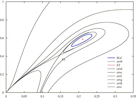
The phase portrait of system (2.5) when λ₁ = 0.05, λ₂ = −0.21.

3. Hopf bifurcation

In this section, we will study the Hopf bifurcation of system (1.3) for some values of model parameters in two cases: (1) R ₀  > 1; (2) Δ  > 0, R ₀  < 1 and 1 +  q  +  pm  < 0.

3.1. In the case that R₀ > 1

From Theorem 1.3, we know that when R ₀  > 1, there is always an unique positive equilibrium (x ^∗,  y ^∗) of (1.3), and (x ^∗,  y ^∗) is a center when S ₂(x ^∗) = 0, where

$$x^{\ast }=\frac{-(1+q+\mathit{pm})+\sqrt{(1+q+\mathit{pm}{)}^2-4\mathit{pn}(p-A)}}{2\mathit{pn}}>0\text{,}{y}^{\ast }={\mathit{qx}}^{\ast }\text{.}$$

Now, we set

$$m=-3\text{,}n=10\text{,}p=9\text{,}q=47\text{,}$$

and substitute them into tr(M ₁(x ^∗)) = 0, thus, we get the equation

$$51674112-12526272A+1221192A^2-66342A^3+1805A^4=0\text{,}$$

which has two real roots A  = 12 and A  = 3738/361. Obviously,

$$m=-3\text{,}n=10\text{,}p=9\text{,}q=47\text{,}A=12\text{,}$$

and

$$m=-3\text{,}n=10\text{,}p=9\text{,}q=47\text{,}A=3738/361\text{.}$$

The two sets of parameter values satisfy the conditions

$$\mathit{tr}(M_1(x^{\ast }))=0\text{,}{R}_0>1\text{,}-2\sqrt{n}<m\text{,}$$

respectively. We first discuss the local property of the unique positive equilibrium (x ^∗,  y ^∗) when (m,  n,  p,  q,  A) = (−3, 10, 9, 47, 12). In this case, we have x ^∗  = 1/10, y ^∗  = 47/10. We consider

$$\begin{array}{cc}\hfill & \frac{\mathrm{d}x}{\mathrm{d}t}=\frac{x}{1-3x+10x^2}(12-x-y)-9x\text{,}\hfill \\ \hfill & \frac{\mathrm{d}y}{\mathrm{d}t}=47x-y\text{.}\hfill \end{array}$$ (3.1)

Lemma 3.1

(1/10,   47/10) is a stable weak focus of multiple one for system (3.1) .

Proof

In order to translate (x ^∗,  y ^∗) to the origin, we set X  =  x  − 1/10, Y  =  y  − 47/10. And we rename X, Y as x, y, respectively. Then (3.1) becomes

$$\begin{array}{cc}\hfill & \frac{\mathrm{d}x}{\mathrm{d}t}=\frac{(x+1/10)}{1-3(x+1/10)+10(x+1/10{)}^2}(72/10-x-y)-9(x+1/10)\text{,}\hfill \\ \hfill & \frac{\mathrm{d}y}{\mathrm{d}t}=47x-y\text{.}\hfill \end{array}$$ (3.2)

Now, we only need to prove that the origin is a stable weak focus of multiple one of (3.2). Using Taylor expansion for (3.2), then we have

$$\begin{array}{cc}\hfill & \frac{\mathrm{d}x}{\mathrm{d}t}=x-\frac{1}{8}y-\frac{45}{32}\mathit{xy}-\frac{25}{128}{x}^{2}y-125x^3+\mathrm{O}(|x\text{,}y{|}^4)\text{,}\hfill \\ \hfill & \frac{\mathrm{d}y}{\mathrm{d}t}=47x-y\text{.}\hfill \end{array}$$ (3.3)

Making the change of variables u  =  x, $v=-\frac{4}{\sqrt{78}}x+\frac{1}{2\sqrt{78}}y$, $\tau =\frac{\sqrt{78}}{4}t$, and rewriting τ as t, we obtain

$$\begin{array}{cc}\hfill & \frac{\mathrm{d}u}{\mathrm{d}t}=-v-\frac{45}{\sqrt{78}}{u}^2-\frac{45}{4}\mathit{uv}-\frac{25}{16}{u}^{2}v-\frac{2025}{4\sqrt{78}}{u}^3+\mathrm{O}(|u\text{,}v{|}^4)\text{,}\hfill \\ \hfill & \frac{\mathrm{d}v}{\mathrm{d}t}=u+\frac{15\sqrt{78}}{26}\mathit{uv}+\frac{30}{13}{u}^2+\frac{25\sqrt{78}}{312}{u}^{2}v+\frac{2025}{78}{u}^3+\mathrm{O}(|u\text{,}v{|}^4)\text{.}\hfill \end{array}$$ (3.4)

Thus, we can get the first Liapounov constant $W_1=-46925\sqrt{78}\mathrm{\pi }/16224<0$. Therefore the origin is a stable weak focus of order one for (3.4). The conclusion follows. □

In the following, we choose A as a bifurcation parameter. Let

$$A=12+{ϵ}_1\text{.}$$

Then we may write (3.1) as follows

$$\begin{array}{cc}\hfill & \frac{\mathrm{d}x}{\mathrm{d}t}=\frac{x}{1-3x+10x^2}(12+{ϵ}_1-x-y)-9x\text{,}\hfill \\ \hfill & \frac{\mathrm{d}y}{\mathrm{d}t}=47x-y\text{.}\hfill \end{array}$$ (3.5)

The positive equilibrium of system (3.5) is $E^{\ast }\left(\frac{-7+\sqrt{169+40{ϵ}_1}}{60}\text{,}\frac{-329+47\sqrt{169+40{ϵ}_1}}{60}\right)$ and the linearizing matrix of (3.5) at E ^∗ is

$$\left(\begin{array}{cc}\hfill {\Lambda }_1\hfill & \hfill {\Lambda }_2\hfill \\ \hfill 47\hfill & \hfill -1\hfill \end{array}\right)\text{,}$$

where

$${\Lambda }_1=\frac{-627-90{ϵ}_1+51\sqrt{169+40{ϵ}_1}}{88+5{ϵ}_1-4\sqrt{169+40{ϵ}_1}}\text{,}{\Lambda }_2=\frac{21-3\sqrt{169+40{ϵ}_1}}{4(88+5{ϵ}_1-4\sqrt{169+40{ϵ}_1})}\text{.}$$

Therefore, the characteristic equation of which is

$${\lambda }^2+(1-{\Lambda }_1)\lambda -{\Lambda }_1-47{\Lambda }_2=0$$

and

$$\lambda =\frac{-(715+95{ϵ}_1-55\sqrt{169+40{ϵ}_1})\pm \mathrm{i}\sqrt{-931190-7225{ϵ}_1^2+78110\sqrt{169+40{ϵ}_1}-{ϵ}_1(227645-9325\sqrt{169+40{ϵ}_1})}}{2(88+5{ϵ}_1-4\sqrt{169+40{ϵ}_1})}\text{.}$$

Obviously, (i) Re  λ(ϵ ₁)∣(ϵ ₁  = 0) = 0, $\mathrm{Im}\lambda ({ϵ}_1)|({ϵ}_1=0)=\frac{\sqrt{65}}{2}\ne 0$; (ii) (Re  λ(ϵ ₁))′(ϵ ₁  = 0) = −15/104 ≠ 0; (iii) from Lemma 3.1, we have W ₁  < 0.

Therefore, by Hopf bifurcation theory, we obtain the following result.

Theorem 3.2

There exists a σ ₁  >  0, and a function ϵ ₁   =   ϵ ₁ (x ₁ ) defined on $0<x_1-\frac{1}{10}⩽{\sigma }_1$ , which satisfies ${ϵ}_1\left(\frac{1}{10}\right)=0$ . And when ϵ ₁   =   ϵ ₁ (x ₁ )  <  0, system (3.5) has a unique stable limit cycle which passes through (x ₁ ,   47/10).

Next we consider system (1.3) when (m,  n,  p,  q,  A) = (−3, 10, 9, 47, 3738/361):

$$\begin{array}{cc}\hfill & \frac{\mathrm{d}x}{\mathrm{d}t}=\frac{x}{1-3x+10x^2}(3738/361-x-y)-9x\text{,}\hfill \\ \hfill & \frac{\mathrm{d}y}{\mathrm{d}t}=47x-y\text{.}\hfill \end{array}$$ (3.6)

In this case system (1.3) has a unique positive equilibrium (x ^∗,  y ^∗), where x ^∗  = 1/19, y ^∗  = 47/19. By the similar arguments for the case (m,  n,  p,  q,  A) = (−3, 10, 9, 47, 12), we obtain that the first Liapounov constant of (1/19, 47/19) is $W_1=-4297376129\mathrm{\pi }/242408\sqrt{181806}<0$. Therefore, we get

Lemma 3.3

(1/19,   47/19) is a stable weak focus of order one for system (3.6) .

In the following, we still choose A as a bifurcation parameter. Let

$$A=3738/361+{ϵ}_2\text{.}$$

Then we can write (3.6) as follows:

$$\begin{array}{cc}\hfill & \frac{\mathrm{d}x}{\mathrm{d}t}=\frac{x}{1-3x+10x^2}(3738/361+{ϵ}_2-x-y)-9x\text{,}\hfill \\ \hfill & \frac{\mathrm{d}y}{\mathrm{d}t}=47x-y\text{.}\hfill \end{array}$$ (3.7)

The positive equilibrium of system (3.7) is $E^{\ast }\left(\frac{-133+\sqrt{37249+14440{ϵ}_2}}{1140}\text{,}\frac{-6251+47\sqrt{37249+14440{ϵ}_2}}{1140}\right)$ and the linearizing matrix of (3.7) at E ^∗ is

$$\left(\begin{array}{cc}\hfill \overline{{\Lambda }_1}\hfill & \hfill \overline{{\Lambda }_2}\hfill \\ \hfill 47\hfill & \hfill -1\hfill \end{array}\right)\text{,}$$

where

$$\overline{{\Lambda }_1}=\frac{172887+32490{ϵ}_2-969\sqrt{37249+14440{ϵ}_2}}{-28798-1805{ϵ}_2+76\sqrt{37249+14440{ϵ}_2}}\text{,}\overline{{\Lambda }_2}=\frac{57(-133+\sqrt{37249+14440{ϵ}_2})}{4(-28798-1805{ϵ}_2+76\sqrt{37249+14440{ϵ}_2})}\text{.}$$

Therefore, the characteristic equation is

$${\lambda }^2+(1-\overline{{\Lambda }_1})\lambda -\overline{{\Lambda }_1}-47\overline{{\Lambda }_2}=0$$

and λ  = Re(λ) ± i Im(λ), where

$$\begin{array}{cc}\hfill & \mathrm{Re}(\lambda )=\frac{201685+34295{ϵ}_2-1045\sqrt{37249+14440{ϵ}_2}}{-57596-3610{ϵ}_2+152\sqrt{37249+14440{ϵ}_2}}\text{,}\hfill \\ \hfill & \mathrm{Im}(\lambda )=\frac{\sqrt{-68310792104-941569225{ϵ}_2^2+361572128\sqrt{37240+14440{ϵ}_2}+1805{ϵ}_2(-13263757+33041\sqrt{37249+14440{ϵ}_2})}}{-57596-3610{ϵ}_2+152\sqrt{37249+14440{ϵ}_2}}\text{.}\hfill \end{array}$$

Obviously, (i) Re(λ)∣(ϵ ₂  = 0) = 0, $\mathrm{Im}(\lambda )|({ϵ}_2=0)=-\sqrt{\frac{579}{314}}\ne 0$; (ii) $(\mathrm{Re}(\lambda ){)}^{\prime }|({ϵ}_2=0)=\frac{20577}{121204}\ne 0$; (iii) from Lemma 3.3, we have W ₁  < 0.

Therefore, by the Hopf bifurcation theory, we obtain

Theorem 3.4

There exists a σ ₂  >  0, and a function ϵ ₂   =   ϵ ₂ (x ₁ ) defined on $0<x_1-\frac{1}{19}⩽{\sigma }_2$ , which satisfies ${ϵ}_2(\frac{1}{19})=0$ . And when ϵ ₂   =   ϵ ₂ (x ₁ )  >  0, system (3.7) has a unique stable limit cycle which passes through (x ₁ ,   47/19).

The bifurcation diagram of system (3.5), (3.7) is in Fig. 3.1 . The bifurcation diagram shows that the unique positive equilibrium (x ^∗,  y ^∗) is unstable when 3738/361 <  A  < 12 and is stable when A  < 3738/361 or A  > 12. Thus Hopf bifurcations occur and there exists a stable limit cycle when 3738/361 <  A  < 12, which are the conclusions in Theorem 3.2, Theorem 3.4. As an example, setting A  = 11, we obtain the phase portrait of system (3.5) or (3.7) (see Fig. 3.2 ).

Fig. 3.1.

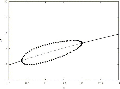
The bifurcation diagram of (3.5) (or (3.7)) by parameter A and the y-coordinate of the limit cycle.

Fig. 3.2.

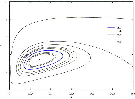
A stable limit cycle of (3.5) when m = −3, n = 10, A = 11, q = 47, p = 9.

3.2. In the case that Δ > 0, R₀ < 1 and 1 + q + pm < 0

From Theorem 1.3, we also know that when Δ  > 0, R ₀  < 1 and 1 +  q  +  pm  < 0, system (1.3) has two positive equilibria E ₁(x ₁,  y ₁) and E ₂(x ₂,  y ₂), and E ₁(x ₁,  y ₁) is a saddle. Furthermore, E ₂(x ₂,  y ₂) is a center when S ₂(x ₂) = 0. The set of number

$$m=-5\text{,}n=18\text{,}p=7\text{,}q=11\text{,}A=6$$

satisfy that

$$\mathrm{tr}{M}_1(x_2)=0\text{,}p>A\text{,}-2\sqrt{n}<m<0\text{.}$$

Now we discuss the local property of the unique positive equilibrium E ₂(x ₂,  y ₂) when (m,  n,  p,  q,  A) = (−5, 18, 7, 11, 6). In this case, we have x ₂  = 1/9, y ₂  = 11/9. We consider

$$\begin{array}{cc}\hfill & \frac{\mathrm{d}x}{\mathrm{d}t}=\frac{x}{1-5x+18x^2}(6-x-y)-7x\text{,}\hfill \\ \hfill & \frac{\mathrm{d}y}{\mathrm{d}t}=11x-y\text{.}\hfill \end{array}$$ (3.8)

By the similar argument as above, we obtain that the first Liapounov constant of system (3.8) about (1/9, 11/9) is $W_1=6831\sqrt{30}\mathrm{\pi }/400>0$. Therefore, we get

Lemma 3.5

(1/9,   11/9) is a unstable weak focus of multiple one of system (3.8) .

In the following, we choose A as a bifurcation parameter. Let

$$A=6+\delta \text{.}$$

Then we may write (3.8) as follows:

$$\begin{array}{cc}\hfill & \frac{\mathrm{d}x}{\mathrm{d}t}=\frac{x}{1-5x+18x^2}(6+\delta -x-y)-7x\text{,}\hfill \\ \hfill & \frac{\mathrm{d}y}{\mathrm{d}t}=11x-y\text{.}\hfill \end{array}$$ (3.9)

The second positive equilibrium of system (3.9) is $E_2\left(\frac{23+\sqrt{25+504\delta }}{252}\text{,}\frac{253+11\sqrt{25+504\delta }}{252}\right)$ and the linearizing matrix of (3.9) at E ₂ is

$$\left(\begin{array}{cc}\hfill \overline{\overline{{\Lambda }_1}}\hfill & \hfill \overline{\overline{{\Lambda }_2}}\hfill \\ \hfill 11\hfill & \hfill -1\hfill \end{array}\right)\text{,}$$

where

$$\overline{\overline{{\Lambda }_1}}=\frac{7(-19+42\delta +\sqrt{25+504\delta })}{-103-21\delta +\sqrt{25+504\delta }}\text{,}\overline{\overline{\delta }}=\frac{7(23+\sqrt{25+504\delta })}{12(-103-21\delta +\sqrt{25+504\delta })}\text{.}$$

Therefore, the characteristic equation is

$${\lambda }^2+(1-\overline{\overline{{\Lambda }_1}})\lambda -\overline{\overline{{\Lambda }_1}}-47\overline{\overline{{\Lambda }_2}}=0$$

and λ  = Re(λ) ± i Im(λ), where

$$\begin{array}{cc}\hfill & \mathrm{Re}(\lambda )=\frac{-90+945\delta +18\sqrt{25+504\delta }}{6(-103-21\delta +\sqrt{25+504\delta })}\text{,}\hfill \\ \hfill & \mathrm{Im}(\lambda )=\frac{\sqrt{-670761{\delta }^2-63\delta (-13723+547\sqrt{25+504\delta })+24(1075+2186\sqrt{25+504\delta })}}{6(-103-21\delta +\sqrt{25+504\delta })}\text{.}\hfill \end{array}$$

Obviously, (i) Re(λ)∣(δ  = 0) = 0, $\mathrm{Im}(\lambda )|(\delta =0)=-\sqrt{\frac{5}{6}}\ne 0$; (ii) $(\mathrm{Re}(\lambda ){)}^{\prime }|(\delta =0)=-\frac{63}{20}\ne 0$; (iii) from Lemma 3.5, we have W ₁  > 0. Thus, by the Hopf bifurcation theory, we obtain the following conclusion.

Theorem 3.6

There exists a σ ₃  >  0, and a function $\delta =\delta (\overline{x_1})$ defined on $0<\overline{x_1}-\frac{1}{9}⩽{\sigma }_3$ , which satisfies $\delta (\frac{1}{9})=0$ . And when $\delta =\delta (\overline{x_1})>0$ system (3.9) has a unique unstable limit cycle which passes through $(\overline{x_1}\text{,}11/9)$ .

Fig. 3.3 show the bifurcation diagram of system (3.9). When δ  ⩽ 0, the positive equilibrium E ₂(x ₂,  y ₂) is unstable focus; when δ  > 0, the stability of the equilibrium E ₂(x ₂,  y ₂) is changed and a Hopf bifurcation occur. Hence, when δ  > 0 the positive equilibrium E ₂(x ₂,  y ₂) is a stable focus and there exists a unstable limit cycle. As an example, setting δ  = 0.008702, we obtain the phase portrait of system (3.9) (see Fig. 3.4 ).

Fig. 3.3.

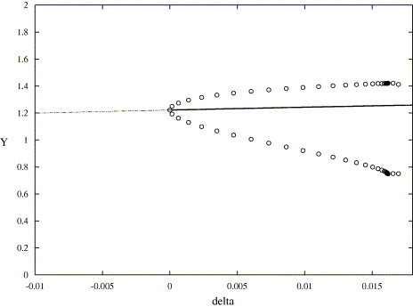
The bifurcation diagram of (3.9) by parameter δ and the y-coordinate of the limit cycle.

Fig. 3.4.

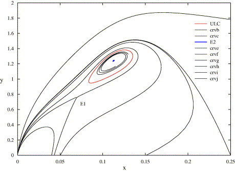
A unstable limit cycle when m = −5, n = 18, A = 6.008702, q = 11, p = 7.

4. Conclusion

Epidemic mathematical models have become important tools to study the transmission dynamics of infectious diseases in host populations. There have been lots of works on the stability of endemic equilibrium for some epidemic models (cf. [10], [11], [12] and references therein). In this paper, we have studied the bifurcation behaviors of the SIR epidemic model with the general non-monotone and nonlinear incidence rate kIS/(1 +  βI  +  αI ²). From the analysis, we have found that there exist some values of the model such that the model can undergo a series of bifurcations, such as saddle-node bifurcation, Hopf bifurcation and Bogdanov–Takens bifurcation. When a stable limit cycle surrounds the endemic equilibrium, it means that the number of the infective tends to a periodic function and the disease will exhibit frequently regular oscillation. Hence, the disease become periodic outbreak as time evolves. On the other hand, there exist some parameters values such that the model has two endemic equilibria (one is a saddle and the other is center-type equilibrium) and a stable homoclinic loop. Thus, the disease will persist.

Communicated by Prof. Iovane

References

- 1.Alexander M.E., Moghadas S.M. Periodicity in an epidemic model with a generalized non-linear incidence. Math Biosci. 2004;189:75–96. doi: 10.1016/j.mbs.2004.01.003. [DOI] [PubMed] [Google Scholar]
- 2.Capasso V., Serio G. A generalization of the Kermack–Mckendrick deterministic epidemic model. Math Biosci. 1978;42:43–61. [Google Scholar]
- 3.Derrick W.R., van den Driessche P. A disease transmission model in a nonconstant population. J Math Biol. 1993;31:495–512. doi: 10.1007/BF00173889. [DOI] [PubMed] [Google Scholar]
- 4.Gumel A.B. Modelling strategies for controlling SARS outbreaks. Proc R Soc Lond B. 2004;271:2223–2232. doi: 10.1098/rspb.2004.2800. [DOI] [PMC free article] [PubMed] [Google Scholar]
- 5.Hethcote H.W. The mathematics of infectious disease. SIAM Rev. 2000;42:599–653. [Google Scholar]
- 7.Hethcote H.W., van den Driessche P. Some epidemiological models with nonlinear incidence. J Math Biol. 1991;29:271–287. doi: 10.1007/BF00160539. [DOI] [PubMed] [Google Scholar]
- 8.Kermack W.O., McKendrick A.G. A contribution to the mathematical theory of epidemics. Proc R Soc Lond. 1927;115:700–721. [Google Scholar]
- 9.Leung G.M. The impact of community psychological response on outbreak control for severe acute respiratory syndrome in Hong Kong. J Epidemiol Community Health. 2003;57:857–863. doi: 10.1136/jech.57.11.857. [DOI] [PMC free article] [PubMed] [Google Scholar]
- 10.Li G.-H., Jin Z. Global stability of an SEI epidemic model. Chaos, Solitons & Fractals. 2004;21:925–931. [Google Scholar]
- 11.Li G.-H., Jin Z. Global stability of an SEI epidemic model with general contact. Chaos, Solitons & Fractals. 2005;23:997–1004. [Google Scholar]
- 12.Li G.-H., Jin Z. Global stability of a SEI epidemic model with infectious force in latent, infected and immune period. Chaos, Solitons & Fractals. 2005;25:1177–1184. [Google Scholar]
- 13.Liu W.M., Hethcote H.W., Levin S.A. Dynamical behavior of epidemiological models with nonlinear incidence rates. J Math Biol. 1987;25:359–380. doi: 10.1007/BF00277162. [DOI] [PubMed] [Google Scholar]
- 14.Liu W.M., Levin S.A., Iwasa Y. Influence of nonlinear incidence rates upon the behavior of SIRS epidemiological models. J Math Biol. 1986;23:187–204. doi: 10.1007/BF00276956. [DOI] [PubMed] [Google Scholar]
- 16.Ruan S., Wang W. Dynamical behavior of an epidemic model with a nonlinear incidence rate. J Different Equat. 2003;188:135–163. [Google Scholar]
- 18.Xiao D-M, Ruan S-G. Global analysis of an epidemic model with a nonlinear incidence rate. Preprint 2005.
- 19.Zhang Z.-F., Ding T.-R., Huang W.-Z., Dong Z.-X. Qualitative theory of differential equations. vol. 101. Amer Math Soc; Providence: 1992. (Translations of mathematical monographs). [Google Scholar]