On the analysis of a multi-regions discrete SIR epidemic model: an optimal control approach

Abstract

In this paper, we devise a discrete time SIR model depicting the spread of infectious diseases in various geographical regions that are connected by any kind of anthropological movement, which suggests disease-affected people can propagate the disease from one region to another via travel. In fact, health policy-makers could manage the problem of the regional spread of an epidemic, by organizing many vaccination campaigns, or by suggesting other defensive strategies such as blocking movement of people coming from borders of regions at high-risk of infection and entering very controlled regions or with insignificant infection rate. Further, we introduce in the discrete SIR systems, two control variables which represent the effectiveness rates of vaccination and travel-blocking operation. We focus in our study to control the outbreaks of an epidemic that affects a hypothetical population belonging to a specific region. Firstly, we analyze the epidemic model when the control strategy is based on the vaccination control only, and secondly, when the travel-blocking control is added. The multi-points boundary value problems, associated to the optimal control problems studied here, are obtained based on a discrete version of Pontryagin’s maximum principle, and resolved numerically using a progressive-regressive discrete scheme that converges following an appropriate test related to the Forward-Backward Sweep Method on optimal control.

Introduction

Mathematical modeling has played important role in describing and analyzing the evolution of infectious diseases. In 1927, Kermack and McKendrick [1] were the first researchers on mathematical epidemiology to propose the SIR model which is one of the classical epidemic models that has a compartment structure. In SIR systems, the host population is divided into three epidemiological groups: the susceptibles (S) (individuals not yet infected with the disease), the infectives (I) (individuals who have been infected with the disease and are capable of spreading the disease to those in the susceptible category), and the removed (R) (individuals who have been infected and then removed from the disease. Those in this category are not able to be infected again or transmit the infection to others). The transmission dynamics of an infectious disease is described by modeling the population movements among those epidemiological compartments. In these types of models, individuals develop an immunity to some diseases such as chicken pox and SARS. In addition, contacts between infected and susceptible individuals can take part in the spread of the epidemic.

On a large geographical scale, the disease becomes spatially mobile to different regions due to the movement of people from a region to another. The infection transport network becomes more complex when people come via airplane for instance, from further places.

The mathematical models conventional of the spread of the disease, have usually ignored or overlooked the spatial dynamics, while the spatial spread of infection has been observed many times [2]. In fact, there exist in the history of infectious diseases, many examples of infection that was observed spreading with respect to space. Sometimes, epidemics spread over large areas, and can even reach continents. Such cases include the Black Death (plague) which emerged in Europe in the 1300s, measles and smallpox in the New World between the 1500s and 1600s, HIV/AIDS in 1981, West Nile virus in North America in the late 1990s, and SARS in Asia in 2003 [3].

The spatial spread of infectious diseases is a phenomenon that involves many different components, which makes its modeling a complex task. Spatial heterogeneity requires a formulation of a small model for each region (city, or state, etc). One possible approach is to consider the travel of individuals between discrete geographical regions (subdomains of domain of study), assuming that the transmission does not take place during travel. For diseases that affect animals and insects (vectors), and can also be passed on to humans [4], it is important to accurately model not only the contact/mixing between humans and the various species, but also the movement patterns of each of the species involved, including humans.

The importance of modelling spatial spread of infectious disease can be highlighted by considering the Ebola outbreaks disease in several sub-Saharan African countries [5]. Before the diagnosis of that disease, infected people moved from one city to another. After some infected cases were diagnosed, and the problem was recognized, it took some time until the political decision was made to ban all movements. At that time, the infected cases had already been divided among a large number of regions. The problem was exacerbated. Then, in order to control the spatial spread of the disease, it has became necessary to consider all parts that people can visit. Hence, this study showcases the significance of integration of spatial dynamics in mathematical models of the spread of infectious diseases.

There is an increasing interest in the study and application of spatial spread [3, 6, 7]. Most of the models studied, have been partly continuous because of their mathematical tractability. In Allen et al. [8], a discrete-time, age-independent SIR type epidemic model with n subgroups is formulated and analyzed, then applied to a measles epidemic on a university campus. In similar pattern, we devise a discrete-time SIR model that describes the propagation of a disease in a population of individuals who travel between p regions (domains).

Figure 1 illustrates an example of discrete geographical domains of region of Casablanca-Settat (Morocco) where $p=9$, that image was originally made based on information from [9]. Births and deaths are included but the population size of each domain remains constant. One reason for the upsurge of discrete epidemic models is that discrete models have advantages in describing an infectious disease since epidemic data are usually collected in discrete time units, which would make it more convenient to use discrete-time models [10] and the ease with which data can be compared to the simulated results [8].

Fig. 1.

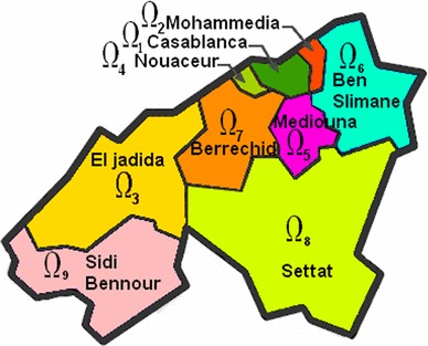
Region of Casablanca-Settat in Morocco. This region is divided into nine subregions (or domains) ${({\mathit{\Omega }}_i)}_{1\le i\le 9}$: Casablanca (${\mathit{\Omega }}_1$), Mohammedia (${\mathit{\Omega }}_2$), El jadida (${\mathit{\Omega }}_3$), Nouaceur (${\mathit{\Omega }}_4$), Mediouna (${\mathit{\Omega }}_5$), Ben Slimane (${\mathit{\Omega }}_6$), Berrechid (${\mathit{\Omega }}_7$), Settat (${\mathit{\Omega }}_8$) and Sidi Bennour (${\mathit{\Omega }}_9$) [9]

In the literature, there have been many studies of discrete epidemic models [11–15] and references therein. In Reference Allen et al. [11], explained the advantage of SIS and SIR discrete-time models in approximating the more well-known continuous-time epidemic models. As regards to the positivity of solutions, discrete-time equations often provide positive solutions. However, differential equations give similar behaviors of solutions when time step is approaching zero [12].

There are different approaches to model the evolution of infectious diseases in discrete time. The recurrent difference equations from the discretisation of continuous differential equation models is one of the direct modeling approaches and frequently used, since this type of model can be well understood in the application under reasonable assumptions knowing that there are limits on the range of parameters [13, 14]. We will use this approach to formulate the model considered in this paper. Optimal control theory is well used as an available and effective option for diseases control, mainly Tuberculosis [16–20], Malaria [21, 22], HIV [23–31], Hepatitis [32, 33], Vector borne diseases [34], Cancer [35–40], and other diseases [41–47], but there are very few applications with both space and time as discrete variables. The aforementioned studies, especially those related to infectious diseases, have mainly focused on the optimization of the intervention for single region, rather than the intervention for multiple regions, hence, this work has a novel control application in addition to providing a framework to analyze spatial control strategies. The aim of this work is not to consider a special disease but to set up an optimal control problem relative to multi-regional discrete-time SIR model, applicable for any type of infectious diseases. Firstly, we represent the percentage of vaccinated susceptible populations as a control function of time in the SIR model corresponding to the targeted region aiming to control. Hence, the purpose of this optimal control (vaccination) strategy is to minimize the infected and susceptible individuals, and to maximize the total number of recovered individuals in that region by using the minimum possible cost of applying this control and simultaneously, to investigate the sensitivity of the susceptible individuals by the control (vaccination). We illustrate how the optimal control theory and the percentage of the vaccination (control) variables can be applied to minimize the susceptible and infected individuals and increase the removed ones.

The importance of taking into account the spatial spread of epidemic, is manifested in showing the influence of infection rates in regions at high-risk on theirs neighbors. Secondly, another control variable is added, characterizing the travel-blocking operation which attempts to block contacts between susceptibles of the controlled region (by vaccination) and infected individuals of domains at high-risk. We derive the optimality system for the multi-regional SIR model with the percentage of vaccinated individuals and travel-blocking operation. Then we find an optimal control strategy for this model and solve numerically this system by using an iterative procedure.

The rest of this paper is organized as follows: We describe the model without controls in Sect. 2. Objective functional and the analysis of optimal control with numerical simulations, for the case when only the vaccination control is used, are given in Sect. 3. Section 4 includes the analysis of optimal control problem and numerical simulations of the case when the travel-blocking control is also added. Finally, we conclude in Sect. 5.

The multi-regions discrete SIR model

We assume that there are p geographical regions (domains) of the domain studied $\mathit{\Omega }$ (In Fig. 1, $\mathit{\Omega }$ is the region of Casabanca-Settat with $p=9$).

Let $\mathit{\Omega }={\bigcup }_{j=1}^p{\mathit{\Omega }}_j$, and let $N_i^{{\mathit{\Omega }}_j}$ be the population of domain ${\mathit{\Omega }}_j$ at time i, i.e., the number of individuals who are physically present in ${\mathit{\Omega }}_j$, both residents and travelers. According to the disease transmission mechanism, the host population of ${\mathit{\Omega }}_j$ is grouped into three epidemiological compartments, let $S_i^{{\mathit{\Omega }}_j}$, $I_i^{{\mathit{\Omega }}_j}$ and $R_i^{{\mathit{\Omega }}_j}$ be the number of individuals in the susceptible, infective, and removed compartments of ${\mathit{\Omega }}_j$ at time i, respectively. In addition to the death and recruitment, there are population movements among those three epidemiological compartments from time unit i to time $i+1$. We assume that the recruited individuals (by birth and immigration) are constant and enter the susceptible compartment. To make the model a little more realistic, but in order to work with a constant overall population, we suppose that birth and death occur with the same rate. In addition, we suppose that individuals who are out of their domain do not give birth, and so birth occurs in the home domain at a per capita rate $d_j>0$. And death takes place anywhere with a per capita rate $d_j$. After one unit time, the susceptible individuals may stay in the susceptible compartment, or get infected and move to the infectious compartment, or die. Disease transmission is assumed to occur between individuals present in a given domain ${\mathit{\Omega }}_j$. The individuals in the infective compartment can keep being the infective, or get recovery and be transferred to the recovered compartment, or die, assuming that there is no mortality due to infection. The individuals in the recovered compartment never leave the compartment unless they die.

The disease transmission in a given domain ${\mathit{\Omega }}_j$ at time i is modelled using standard incidence, given by

$$\begin{array}{c}\hfill \sum _{k=1}^p{\mathit{\beta }}_{jk}\frac{I_i^{{\mathit{\Omega }}_k}}{N_i^{{\mathit{\Omega }}_j}}{S}_i^{{\mathit{\Omega }}_j}\end{array}$$

where the disease transmission coefficient ${\mathit{\beta }}_{jk}>0$ is the proportion of adequate contacts in domain ${\mathit{\Omega }}_j$ between a susceptible from ${\mathit{\Omega }}_j$ and an infective from another domain ${\mathit{\Omega }}_k$.

The multi-regions discrete-time SIR model associated to ${\mathit{\Omega }}_j$ is written as follows

$$\begin{array}{cc}\hfill S_{i+1}^{{\mathit{\Omega }}_j}=& S_i^{{\mathit{\Omega }}_j}-\sum _{k=1}^p{\mathit{\beta }}_{jk}\frac{I_i^{{\mathit{\Omega }}_k}}{N_i^{{\mathit{\Omega }}_j}}{S}_i^{{\mathit{\Omega }}_j}+\left(N_i^{{\mathit{\Omega }}_j}-S_i^{{\mathit{\Omega }}_j}\right)d_j\hfill \end{array}$$ 1

$$\begin{array}{cc}\hfill I_{i+1}^{{\mathit{\Omega }}_j}=& I_i^{{\mathit{\Omega }}_j}+\sum _{k=1}^p{\mathit{\beta }}_{jk}\frac{I_i^{{\mathit{\Omega }}_k}}{N_i^{{\mathit{\Omega }}_j}}{S}_i^{{\mathit{\Omega }}_j}-{\mathit{\gamma }}_j{I}_i^{{\mathit{\Omega }}_j}-d_j{I}_i^{{\mathit{\Omega }}_j}\hfill \end{array}$$ 2

$$\begin{array}{cc}\hfill R_{i+1}^{{\mathit{\Omega }}_j}=& R_i^{{\mathit{\Omega }}_j}+{\mathit{\gamma }}_j{I}_i^{{\mathit{\Omega }}_j}-d_j{R}_i^{{\mathit{\Omega }}_j}\hfill \end{array}$$ 3

where $d_j$ is the birth and death rate and ${\mathit{\gamma }}_j$ is the recovery rate. The biological background requires that all parameters be non-negative.

$N_i^{{\mathit{\Omega }}_j}=S_i^{{\mathit{\Omega }}_j}+I_i^{{\mathit{\Omega }}_j}+R_i^{{\mathit{\Omega }}_j}$ is the population size corresponding to domain ${\mathit{\Omega }}_j$ at time i. It is clear that the population size remains constant for all $i\ge 0$, in fact

$$\begin{array}{cc}\hfill N_{i+1}^{{\mathit{\Omega }}_j}=& S_{i+1}^{{\mathit{\Omega }}_j}+I_{i+1}^{{\mathit{\Omega }}_j}+R_{i+1}^{{\mathit{\Omega }}_j}\hfill \\ \hfill =& S_i^{{\mathit{\Omega }}_j}+I_i^{{\mathit{\Omega }}_j}+R_i^{{\mathit{\Omega }}_j}+d_j{N}_i^{{\mathit{\Omega }}_j}-d_j\hfill \\ \hfill & \times \left(S_i^{{\mathit{\Omega }}_j}+I_i^{{\mathit{\Omega }}_j}+R_i^{{\mathit{\Omega }}_j}\right)=N_i^{{\mathit{\Omega }}_j}\hfill \end{array}$$

The model with vaccination only

Presentation of the model

We introduce a control variable $u_i^{{\mathit{\Omega }}_j}$ that characterizes the effectiveness of treatment (vaccination) in the above mentioned model (1–3). Then, for a given region ${\mathit{\Omega }}_j$ the model is given by the following equations:

$$\begin{array}{cc}\hfill S_{i+1}^{{\mathit{\Omega }}_j}=& S_i^{{\mathit{\Omega }}_j}-\sum _{k=1}^p{\mathit{\beta }}_{jk}\frac{I_i^{{\mathit{\Omega }}_k}}{N_i^{{\mathit{\Omega }}_j}}{S}_i^{{\mathit{\Omega }}_j}+\left(N_i^{{\mathit{\Omega }}_j}-S_i^{{\mathit{\Omega }}_j}\right)d_j\hfill \\ \hfill & -u_i^{{\mathit{\Omega }}_j}{S}_i^{{\mathit{\Omega }}_j}\hfill \end{array}$$ 4

$$\begin{array}{cc}\hfill I_{i+1}^{{\mathit{\Omega }}_j}=& I_i^{{\mathit{\Omega }}_j}+\sum _{k=1}^p{\mathit{\beta }}_{jk}\frac{I_i^{{\mathit{\Omega }}_k}}{N_i^{{\mathit{\Omega }}_j}}{S}_i^{{\mathit{\Omega }}_j}-{\mathit{\gamma }}_j{I}_i^{{\mathit{\Omega }}_j}-d_j{I}_i^{{\mathit{\Omega }}_j}\hfill \end{array}$$ 5

$$\begin{array}{cc}\hfill R_{i+1}^{{\mathit{\Omega }}_j}=& R_i^{{\mathit{\Omega }}_j}+{\mathit{\gamma }}_j{I}_i^{{\mathit{\Omega }}_j}-d_j{R}_i^{{\mathit{\Omega }}_j}+u_i^{{\mathit{\Omega }}_j}{S}_i^{{\mathit{\Omega }}_j}\hfill \end{array}$$ 6

Our goal is obviously to try to minimize the population of the susceptible group and the cost of treatment, while increasing the population in the removed group. Our control function is assumed taking values between $u_{min}^{{\mathit{\Omega }}_j}$ and $u_{max}^{{\mathit{\Omega }}_j}$ , where $u_{max}^{{\mathit{\Omega }}_j}<1$ and $u_{min}^{{\mathit{\Omega }}_j}>0$, $\forall j=1,\dots ,p$.

An optimal control approach

We are interested in controlling the population of region ${\mathit{\Omega }}_j$. Then, the problem is to minimize the objective functional given by

$$\begin{array}{cc}\hfill J_j\left(u^{{\mathit{\Omega }}_j}\right)=& \left({\mathit{\alpha }}_j^I{I}_N^{{\mathit{\Omega }}_j}-{\mathit{\alpha }}_j^R{R}_N^{{\mathit{\Omega }}_j}\right)\hfill \\ \hfill & +\sum _{i=1}^{N-1}\left({\mathit{\alpha }}_j^I{I}_i^{{\mathit{\Omega }}_j}-{\mathit{\alpha }}_j^R{R}_i^{{\mathit{\Omega }}_j}+\frac{A_j}{2}{\left(u_i^{{\mathit{\Omega }}_j}\right)}^2\right)\hfill \end{array}$$ 7

where $A_j>0,{\mathit{\alpha }}_j^I>0,{\mathit{\alpha }}_j^R>0$ are the weight constants of control, the infected and the removed group respectively, and $u^{{\mathit{\Omega }}_j}=\left(u_0^{{\mathit{\Omega }}_j},\dots ,u_{N-1}^{{\mathit{\Omega }}_j}\right)$. Our goal is to minimize the infected group, minimize the systemic costs attempting to increase the number of the removed individuals in ${\mathit{\Omega }}_j$. In other words, we are seeking an optimal control $u^{{\mathit{\Omega }}_j\ast }$ such that

$$\begin{array}{c}\hfill J_j\left(u^{{\mathit{\Omega }}_j\ast }\right)=min\left\{J_j\left(u^{{\mathit{\Omega }}_j}\right)/u^{{\mathit{\Omega }}_j}\in U_j\right\}\end{array}$$

where $U_j$ is the control set defined by

$$\begin{array}{c}\hfill U_j=\left\{u^{{\mathit{\Omega }}_j}\text{measurable}/u_{min}^{{\mathit{\Omega }}_j}\le u_i^{{\mathit{\Omega }}_j}\le u_{max}^{{\mathit{\Omega }}_j}\right\}\end{array}$$

$i=0,\dots ,N-1$

The sufficient condition for existence of an optimal control for the problem follows from Theorem 1 in [48], and at the same time, by using the Pontryagin’s Maximum Principle [49] we derive necessary conditions for our optimal control. For this purpose, we define the Hamiltonian as:

$$\begin{array}{cc}& \mathcal{H}\left({\mathit{\Omega }}_j\right)={\mathit{\alpha }}_j^I{I}_i^{{\mathit{\Omega }}_j}-{\mathit{\alpha }}_j^R{R}_i^{{\mathit{\Omega }}_j}+\frac{A_j}{2}{\left(u_i^{{\mathit{\Omega }}_j}\right)}^2+{\mathit{\zeta }}_{1,i+1}^j\hfill \\ \hfill & \times \left[S_i^{{\mathit{\Omega }}_j}-\sum _{k=1}^p{\mathit{\beta }}_{jk}\frac{I_i^{{\mathit{\Omega }}_k}}{N_i^{{\mathit{\Omega }}_j}}{S}_i^{{\mathit{\Omega }}_j}+\left(N_i^{{\mathit{\Omega }}_j}-S_i^{{\mathit{\Omega }}_j}\right)d_j-u_i^{{\mathit{\Omega }}_j}{S}_i^{{\mathit{\Omega }}_j}\right]\hfill \\ \hfill & +{\mathit{\zeta }}_{2,i+1}^j\left[I_i^{{\mathit{\Omega }}_j}+\sum _{k=1}^p{\mathit{\beta }}_{jk}\frac{I_i^{{\mathit{\Omega }}_k}}{N_i^{{\mathit{\Omega }}_j}}{S}_i^{{\mathit{\Omega }}_j}-{\mathit{\gamma }}_j{I}_i^{{\mathit{\Omega }}_j}-d_j{I}_i^{{\mathit{\Omega }}_j}\right]\hfill \\ \hfill & +{\mathit{\zeta }}_{3,i+1}^j\left[R_i^{{\mathit{\Omega }}_j}+{\mathit{\gamma }}_j{I}_i^{{\mathit{\Omega }}_j}-d_j{R}_i^{{\mathit{\Omega }}_j}+u_i^{{\mathit{\Omega }}_j}{S}_i^{{\mathit{\Omega }}_j}\right]\hfill \end{array}$$ 8

Theorem 3.2.1

(Sufficient conditions) For the optimal control problem given by (7) along with the state Eqs. (4)–(6), there exists a control $u^{{\mathit{\Omega }}_j\ast }\in U_j$ such that

$$\begin{array}{c}\hfill J_j\left(u^{{\mathit{\Omega }}_j\ast }\right)=min\left\{J_j\left(u^{{\mathit{\Omega }}_j}\right)/u^{{\mathit{\Omega }}_j}\in U_j\right\}\end{array}$$

Proof

See Dabbs ([48], Theorem 1). $\square$

Theorem 3.2.2

(Necessary Conditions) Given an optimal control $u^{{\mathit{\Omega }}_j\ast }$ and solutions $S^{{\mathit{\Omega }}_j\ast },I^{{\mathit{\Omega }}_j\ast }\text{and}{R}^{{\mathit{\Omega }}_j\ast }$, there exist ${\mathit{\zeta }}_{k,i}^j,i=1\dots N,k=1,2,3$, the adjoint variables satisfying the following equations:

$$\begin{array}{cc}\hfill {\mathit{\zeta }}_{1,i}^j=& -\left[\left(1-\sum _{k=1}^p{\mathit{\beta }}_{jk}\frac{I_i^{{\mathit{\Omega }}_k\ast }}{N_i^{{\mathit{\Omega }}_j}}-d_j-u_i^{{\mathit{\Omega }}_j\ast }\right){\mathit{\zeta }}_{1,i+1}^j\right.\hfill \\ \hfill & +\left.\sum _{k=1}^p{\mathit{\beta }}_{jk}\frac{I_i^{{\mathit{\Omega }}_k\ast }}{N_i^{{\mathit{\Omega }}_j}}{\mathit{\zeta }}_{2,i+1}^j+u_i^{{\mathit{\Omega }}_j\ast }{\mathit{\zeta }}_{3,i+1}^j\right]\hfill \end{array}$$ 9

$$\begin{array}{cc}\hfill {\mathit{\zeta }}_{2,i}^j=& -\left[{\mathit{\alpha }}_j^I-{\mathit{\beta }}_{jj}\frac{S_i^{{\mathit{\Omega }}_j\ast }}{N_i^{{\mathit{\Omega }}_j}}{\mathit{\zeta }}_{1,i+1}^j\right.\hfill \\ \hfill & +\left.\left(1+{\mathit{\beta }}_{jj}\frac{S_i^{{\mathit{\Omega }}_j\ast }}{N_i^{{\mathit{\Omega }}_j}}-{\mathit{\gamma }}_j-d_j\right){\mathit{\zeta }}_{2,i+1}^j+{\mathit{\gamma }}_j{\mathit{\zeta }}_{3,i+1}^j\right]\hfill \end{array}$$ 10

$$\begin{array}{cc}\hfill {\mathit{\zeta }}_{3,i}^j=& -\left[-{\mathit{\alpha }}_j^R+\left(1-d_j\right){\mathit{\zeta }}_{3,i+1}^j\right]\hfill \end{array}$$ 11

where ${\mathit{\zeta }}_{1,N}^j=0,{\mathit{\zeta }}_{2,N}^j={\mathit{\alpha }}_j^I,{\mathit{\zeta }}_{3,N}^j=-{\mathit{\alpha }}_j^R$, are the transversality conditions. In addition

$$\begin{array}{c}\hfill u_i^{{\mathit{\Omega }}_j\ast }=min\left\{max\left\{u_{min}^{{\mathit{\Omega }}_j},\frac{\left({\mathit{\zeta }}_{1,i+1}^j-{\mathit{\zeta }}_{3,i+1}^j\right)S_i^{{\mathit{\Omega }}_j}}{A_j}\right\},u_{max}^{{\mathit{\Omega }}_j}\right\},\\ \hfill \end{array}$$ 12

$i=0,\dots ,N-1$

Proof

Using Pontryagin’s Maximum Principle [49], and setting $S^{{\mathit{\Omega }}_j}=S^{{\mathit{\Omega }}_j\ast }$, $I^{{\mathit{\Omega }}_j}=I^{{\mathit{\Omega }}_j\ast }$, $R^{{\mathit{\Omega }}_j}=R^{{\mathit{\Omega }}_j\ast }$ and $u^{{\mathit{\Omega }}_j}=u^{{\mathit{\Omega }}_j\ast }$ we obtain the following adjoint equations:

$$\begin{array}{cc}\hfill {\mathit{\zeta }}_{1,i}^j=& -\frac{\mathit{\partial }\mathcal{H}}{\mathit{\partial }{S}_i^{{\mathit{\Omega }}_j}}\hfill \\ \hfill =& -\left[\left(1-\sum _{k=1}^p{\mathit{\beta }}_{jk}\frac{I_i^{{\mathit{\Omega }}_k}}{N_i^{{\mathit{\Omega }}_j}}-d_j-u_i^{{\mathit{\Omega }}_j}\right){\mathit{\zeta }}_{1,i+1}^j\right.\hfill \\ \hfill & +\left.\sum _{k=1}^p{\mathit{\beta }}_k\frac{I_i^{{\mathit{\Omega }}_k}}{N_i^{{\mathit{\Omega }}_j}}{\mathit{\zeta }}_{2,i+1}^j+u_i^{{\mathit{\Omega }}_j}{\mathit{\zeta }}_{3,i+1}^j\right]\hfill \\ \hfill {\mathit{\zeta }}_{2,i}^j=& -\frac{\mathit{\partial }\mathcal{H}}{\mathit{\partial }{I}_i^{{\mathit{\Omega }}_j}}=-\left[{\mathit{\alpha }}_j^I-{\mathit{\beta }}_{jj}\frac{S_i^{{\mathit{\Omega }}_j}}{N_i^{{\mathit{\Omega }}_j}}{\mathit{\zeta }}_{1,i+1}^j\right.\hfill \\ \hfill & +\left.\left(1+{\mathit{\beta }}_{jj}\frac{S_i^{{\mathit{\Omega }}_j}}{N_i^{{\mathit{\Omega }}_j}}-{\mathit{\gamma }}_j-d_j\right){\mathit{\zeta }}_{2,i+1}^j+\mathit{\gamma }{\mathit{\zeta }}_{3,i+1}^j\right]\hfill \\ \hfill {\mathit{\zeta }}_{3,i}^j=& -\frac{\mathit{\partial }\mathcal{H}}{\mathit{\partial }{R}_i^{{\mathit{\Omega }}_j}}\hfill \\ \hfill =& -\left[-{\mathit{\alpha }}_j^R+\left(1-d_j\right){\mathit{\zeta }}_{3,i+1}^j\right]\hfill \end{array}$$

with ${\mathit{\zeta }}_{1,N}^j=0,{\mathit{\zeta }}_{2,N}^j={\mathit{\alpha }}_j^I,{\mathit{\zeta }}_{3,N}^j=-{\mathit{\alpha }}_j^R$. To obtain the optimality conditions we take the variation with respect to control $u_i^{{\mathit{\Omega }}_j}$ and set it equal to zero

$$\begin{array}{c}\hfill \frac{\mathit{\partial }\mathcal{H}}{\mathit{\partial }{u}_i^{{\mathit{\Omega }}_j}}=A_j{u}_i^{{\mathit{\Omega }}_j}-{\mathit{\zeta }}_{1,i+1}^j{S}_i^{{\mathit{\Omega }}_j}+{\mathit{\zeta }}_{3,i+1}^j{S}_i^{{\mathit{\Omega }}_j}=0\end{array}$$

Then we obtain the optimal control

$$\begin{array}{c}\hfill u_i^{{\mathit{\Omega }}_j}=\frac{\left({\mathit{\zeta }}_{1,i+1}^j-{\mathit{\zeta }}_{3,i+1}^j\right)S_i^{{\mathit{\Omega }}_j}}{A_j}\end{array}$$

By the bounds in $U_j$ of the control, it is easy to obtain $u^{{\mathit{\Omega }}_j\ast }$ in the following form

$$\begin{array}{c}\hfill u_i^{{\mathit{\Omega }}_j\ast }=min\left\{max\left\{u_{min}^{{\mathit{\Omega }}_j},\frac{\left({\mathit{\zeta }}_{1,i+1}^j-{\mathit{\zeta }}_{3,i+1}^j\right)S_i^{{\mathit{\Omega }}_j}}{A_j}\right\},u_{max}^{{\mathit{\Omega }}_j}\right\},\end{array}$$

$i=0,\dots ,N-1$ $\square$

Numerical results

We now present numerical simulations associated to the above mentioned optimal control problem. We write a code in $\text{MATLAB}{}^{\mathrm{TM}}$ and simulated our results using different data. The optimality systems is solved based on an iterative discrete scheme that converges following an appropriate test similar the one related to the Forward-Backward Sweep Method (FBSM). The state system with an initial guess is solved forward in time and then the adjoint system is solved backward in time because of the transversality conditions. Afterwards, we update the optimal control values using the values of state and costate variables obtained at the previous steps. Finally, we execute the previous steps till a tolerance criterion is reached.

The multi-regions SIR epidemic model we suggest here, is applicable for any number of regions p. For an example, and in order to show the importance of our work, we choose $p=3$ i.e, we consider three regions (domains) ${\mathit{\Omega }}_1$, ${\mathit{\Omega }}_2$ and ${\mathit{\Omega }}_3$ with different parameters cited in Table 1. We try to control ${\mathit{\Omega }}_1$ by the vaccination term $u^{{\mathit{\Omega }}_1}$ given by (12).

Table 1.

Parameters values of $\mathit{\beta },d$ and $\mathit{\gamma }$ utilized for the resolution of all multi-regions discrete systems (1)–(3), (4)–(6) and (15)–(17), and then leading to simulations obtained from Figs. 2, 3, 4, 5, 6, 7, 8, 9, 10, 11 and 12, with the initial conditions $S_0,I_0$ and $R_0$ associated to the three regions ${\mathit{\Omega }}_1,{\mathit{\Omega }}_2$ and ${\mathit{\Omega }}_3$

	$S_0$	$I_0$	$R_0$	$\mathit{\beta }$	d	$\mathit{\gamma }$
${\mathit{\Omega }}_1$	10,000	900	0	0.051	0.16	0.0025
${\mathit{\Omega }}_2$	8000	900	0	0.2481	0.1346	0.003
${\mathit{\Omega }}_3$	7000	50	0	0.11	0.219	0.025

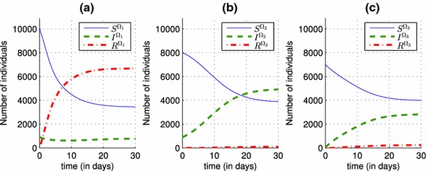
In Fig. 2, we can observe that in the absence of a control and in the presence of an epidemic that spreads in three regions characterized by different parameters, the number of infected individuals rise from $I_0^{{\mathit{\Omega }}_1}=900$, $I_0^{{\mathit{\Omega }}_2}=900$ and $I_0^{{\mathit{\Omega }}_3}=50$ as initial conditions to 5730, 5430 and 3200 in the three regions respectively. Once a vaccination control is introduced in the system (4)–(6), particularly in the equations that describes dynamics of $S^{{\mathit{\Omega }}_1}$, $I^{{\mathit{\Omega }}_1}$ and $R^{{\mathit{\Omega }}_1}$ functions associated to the first region, we can deduce its effect on decreasing the number of infected people in Fig. 3, from 5730 when there was yet no vaccination strategy, to 2750 when there is the control $u^{{\mathit{\Omega }}_1}$. One of the major benefits of that control, is to increase the number of the removed people, and this can be observed in the case (a) of Fig. 3, where the number of the removed people becomes approximately equal to 5500, and that can obviously prove the effectiveness of the vaccination strategy in the first region with a rate that varies in Fig. 4, from a value equal to 0.15 towards a value equal to 0.3, and which also proves that by a control taking only a nonzero value close to 0, we can reach our goal with a significant number of the removed people.

Fig. 2.

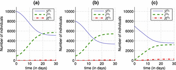
Shapes of state functions of the discrete system (1)–(3) where there is yet no control. a State variables S, I and R associated to the region ${\mathit{\Omega }}_1$. b State variables S, I and R associated to the region ${\mathit{\Omega }}_2$. c State variables S, I and R associated to the region ${\mathit{\Omega }}_3$

Fig. 3.

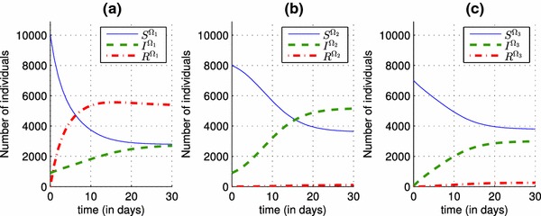
Shapes of state functions of the discrete system (4)–(6) when the control $u^{{\mathit{\Omega }}_1\ast }$ is now introduced. given by (12). a Optimal state variables $S^{\ast },I^{\ast }$ and $R^{\ast }$ associated to the region ${\mathit{\Omega }}_1$. b Optimal state variables $S^{\ast },I^{\ast }$ and $R^{\ast }$ associated to the region ${\mathit{\Omega }}_2$. c Optimal state variables $S^{\ast },I^{\ast }$ and $R^{\ast }$ associated to the region ${\mathit{\Omega }}_3$

Fig. 4.

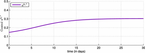
Shape of the optimal control function $u^{{\mathit{\Omega }}_1\ast }$ showing the values taken by the effectiveness rate of the vaccination in the first region ${\mathit{\Omega }}_1$ during one month

We observe in Fig. 5 that the more the control severity weight $A_1$ is small, the control $u^{{\mathit{\Omega }}_1}$ is more important and then there is an increasing of the number of removed people in (a), because $A_1$ has obviously an impact on the values of the control $u^{{\mathit{\Omega }}_1}$ (see simulation (b)) from the control characterization (12), and also these results are obtained from the fact that the most important role of the vaccination control $u^{{\mathit{\Omega }}_1}$ is to increase the number of the removed people $R^{{\mathit{\Omega }}_1}$.

Fig. 5.

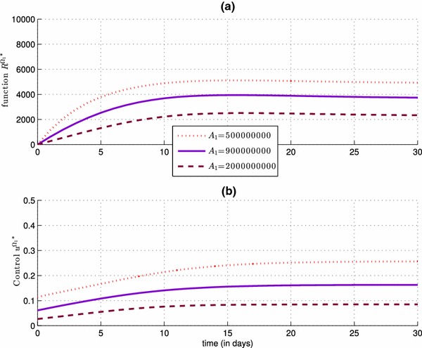
Impact of the control severity weight $A_1$ on the number of the removed people of ${\mathit{\Omega }}_1$ (a), and also on the values of the control $u^{{\mathit{\Omega }}_1}$ (b)

Figure 6 is added here, to show the importance of another control associated to a travel-blocking operation, instead of following only a vaccination strategy. In fact, the number of infected people in ${\mathit{\Omega }}_1$ is increased by hosting people coming from ${\mathit{\Omega }}_2$, and we can see the impact of the infection rate ${\mathit{\beta }}_{12}$ on the system (1)–(3) of ${\mathit{\Omega }}_1$ in Fig. 6, and we deduce that the more ${\mathit{\beta }}_{12}$ is big, the more the number of infected people in the first region becomes huge.

Fig. 6.

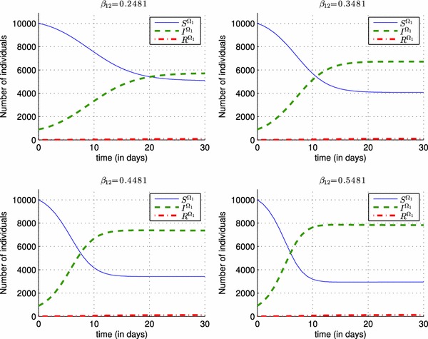
Impact of different values of the infection rate ${\mathit{\beta }}_{12}$ on the shape of the state functions S(t), I(t) and R(t) in region ${\mathit{\Omega }}_1$

The model with vaccination and travel-blocking

Presentation of the model

Let $I=\left\{1,\dots ,p\right\}$, and denote by $I_H\subset I$, the set of indexes of domains at high-risk. We introduce a control variable $v_i^{j{\mathit{\Omega }}_k}$ that characterizes the travel-blocking operation, in order to restrict movements from domains ${\mathit{\Omega }}_k,k\in I_H$ to ${\mathit{\Omega }}_j$. Where

$$\begin{array}{c}\hfill \left\{\begin{array}{ccc}{v}_i^{j{\mathit{\Omega }}_k}<1\hfill & \forall k\in I_H& k\ne j\\ v_i^{j{\mathit{\Omega }}_k}=1\hfill & \text{elsewhere}\\ \forall i\ge 0\hfill \end{array}\right.\end{array}$$ 13

Then for a given region ${\mathit{\Omega }}_j$ the model is given as follows:

$$\begin{array}{cc}\hfill S_{i+1}^{{\mathit{\Omega }}_j}=& S_i^{{\mathit{\Omega }}_j}-\sum _{k=1}^p{v}_i^{j{\mathit{\Omega }}_k}{\mathit{\beta }}_{jk}\frac{I_i^{{\mathit{\Omega }}_k}}{N_i^{{\mathit{\Omega }}_j}}{S}_i^{{\mathit{\Omega }}_j}\hfill \\ \hfill & +\left(N_i^{{\mathit{\Omega }}_j}-S_i^{{\mathit{\Omega }}_j}\right)d_j-u_i^{{\mathit{\Omega }}_j}{S}_i^{{\mathit{\Omega }}_j}\hfill \end{array}$$ 14

$$\begin{array}{cc}\hfill I_{i+1}^{{\mathit{\Omega }}_j}=& I_i^{{\mathit{\Omega }}_j}+\sum _{k=1}^p{v}_i^{j{\mathit{\Omega }}_k}{\mathit{\beta }}_{jk}\frac{I_i^{{\mathit{\Omega }}_k}}{N_i^{{\mathit{\Omega }}_j}}{S}_i^{{\mathit{\Omega }}_j}-{\mathit{\gamma }}_j{I}_i^{{\mathit{\Omega }}_j}-d_j{I}_i^{{\mathit{\Omega }}_j}\hfill \end{array}$$ 15

$$\begin{array}{c}\\ \hfill R_{i+1}^{{\mathit{\Omega }}_j}=& R_i^{{\mathit{\Omega }}_j}+{\mathit{\gamma }}_j{I}_i^{{\mathit{\Omega }}_j}-d_j{R}_i^{{\mathit{\Omega }}_j}+u_i^{{\mathit{\Omega }}_j}{S}_i^{{\mathit{\Omega }}_j}\hfill \end{array}$$ 16

An optimal control approach

The problem is to minimize the objective functional given by

$$\begin{array}{cc}\hfill J_j\left(u^{{\mathit{\Omega }}_j},v^{j{\mathit{\Omega }}_k}\right)=& \left({\mathit{\alpha }}_j^I{I}_N^{{\mathit{\Omega }}_j}-{\mathit{\alpha }}_j^R{R}_N^{{\mathit{\Omega }}_j}\right)\hfill \\ \hfill & +\sum _{k\in I_H}\sum _{i=1}^{N-1}\left({\mathit{\alpha }}_j^I{I}_i^{{\mathit{\Omega }}_j}-{\mathit{\alpha }}_j^R{R}_i^{{\mathit{\Omega }}_j}\right.\hfill \\ \hfill & +\left.\frac{A_j}{2}{\left(u_i^{{\mathit{\Omega }}_j}\right)}^2+\frac{B_k}{2}{\left(v_i^{j{\mathit{\Omega }}_k}\right)}^2\right)\hfill \end{array}$$ 17

where $A_j>0,B_k>0,{\mathit{\alpha }}_j^I>0,{\mathit{\alpha }}_j^R>0$ are the weight constants of controls, the infected and the recovered respectively, $u^{{\mathit{\Omega }}_j}=\left(u_0^{{\mathit{\Omega }}_j},\dots ,u_{N-1}^{{\mathit{\Omega }}_j}\right)$, $v^{j{\mathit{\Omega }}_k}={\left(v^{j{\mathit{\Omega }}_k}\right)}_{k\in I_H}$ and $v^{j{\mathit{\Omega }}_k}=\left(v_0^{j{\mathit{\Omega }}_k},\dots ,v_{N-1}^{j{\mathit{\Omega }}_k}\right)$.

Our goal is to minimize the infected group, minimize the cost of applying controls and increase the number of recovered in ${\mathit{\Omega }}_j$.

In other words, we are seeking optimal controls $u^{{\mathit{\Omega }}_j\ast }$ and $v^{j{\mathit{\Omega }}_k\ast }$ such that

$$\begin{array}{cc}& J_j\left(u^{{\mathit{\Omega }}_j\ast },v^{j{\mathit{\Omega }}_k\ast }\right)\hfill \\ \hfill & =min\left\{J_j\left(u^{{\mathit{\Omega }}_j},v^{j{\mathit{\Omega }}_k}\right)/u^{{\mathit{\Omega }}_j}\in U_j,v^{j{\mathit{\Omega }}_k}\in V_j\right\}\hfill \end{array}$$

where $U_j$ and $V_j$ are the control sets defined by

$$\begin{array}{cc}\hfill U_j=& \left\{u^{{\mathit{\Omega }}_j}\text{measurable}/u_{min}^{{\mathit{\Omega }}_j}\le u_i^{{\mathit{\Omega }}_j}\right.\hfill \\ \hfill & \left.\le u_{max}^{{\mathit{\Omega }}_j},i=0,\dots ,N-1\right\}\hfill \end{array}$$ 18

$$\begin{array}{cc}\hfill V_j=& \left\{v^{j{\mathit{\Omega }}_l}\text{measurable}/v_{min}^{j{\mathit{\Omega }}_l}\right.\hfill \\ \hfill & \left.\le v_i^{j{\mathit{\Omega }}_l}\le v_{max}^{j{\mathit{\Omega }}_l},i=0,\dots ,N-1,l\in I_H\right\}\hfill \end{array}$$ 19

where $u_{max}^{{\mathit{\Omega }}_j}<1,v_{max}^{j{\mathit{\Omega }}_k}<1$ and $u_{min}^{{\mathit{\Omega }}_j}>0,v_{min}^{j{\mathit{\Omega }}_k}>0$, $\forall k\in I_H$.

By using Pontryagin’s Maximum Principle, [49] we derive necessary conditions for our optimal controls. For this purpose, we define the Hamiltonian as:

$$\begin{array}{cc}\hfill \mathcal{H}\left({\mathit{\Omega }}_j\right)=& \sum _{l\in I_H}{\mathit{\alpha }}_j^I{I}_i^{{\mathit{\Omega }}_j}-{\mathit{\alpha }}_j^R{R}_i^{{\mathit{\Omega }}_j}+\frac{A_j}{2}{\left(u_i^{{\mathit{\Omega }}_j}\right)}^2+\frac{B_l}{2}{\left(v_i^{j{\mathit{\Omega }}_l}\right)}^2\hfill \\ \hfill & +{\mathit{\zeta }}_{1,i+1}^j\left[S_i^{{\mathit{\Omega }}_j}-\sum _{k=1}^p{v}_i^{j{\mathit{\Omega }}_k}{\mathit{\beta }}_{jk}\frac{I_i^{{\mathit{\Omega }}_k}}{N_i^{{\mathit{\Omega }}_j}}{S}_i^{{\mathit{\Omega }}_j}\right.\hfill \\ \hfill & \left.+\left(N_i^{{\mathit{\Omega }}_j}-S_i^{{\mathit{\Omega }}_j}\right)d_j-u_i^{{\mathit{\Omega }}_j}{S}_i^{{\mathit{\Omega }}_j}\right]\hfill \\ \hfill & +{\mathit{\zeta }}_{2,i+1}^j\left[I_i^{{\mathit{\Omega }}_j}+\sum _{k=1}^p{v}_i^{j{\mathit{\Omega }}_k}{\mathit{\beta }}_{jk}\frac{I_i^{{\mathit{\Omega }}_k}}{N_i^{{\mathit{\Omega }}_j}}{S}_i^{{\mathit{\Omega }}_j}\right.\hfill \\ \hfill & \left.-{\mathit{\gamma }}_j{I}_i^{{\mathit{\Omega }}_j}-d_j{I}_i^{{\mathit{\Omega }}_j}\right]\hfill \\ \hfill & +{\mathit{\zeta }}_{3,i+1}^j\left[R_i^{{\mathit{\Omega }}_j}+{\mathit{\gamma }}_j{I}_i^{{\mathit{\Omega }}_j}-d_j{R}_i^{{\mathit{\Omega }}_j}+u_i^{{\mathit{\Omega }}_j}{S}_i^{{\mathit{\Omega }}_j}\right]\hfill \end{array}$$ 20

Theorem 4.2.1

Given optimal controls $u^{{\mathit{\Omega }}_j\ast },v^{j{\mathit{\Omega }}_k\ast }$, $k\in I_H$ and solutions $S^{{\mathit{\Omega }}_j\ast },I^{{\mathit{\Omega }}_j\ast }\text{and}{R}^{{\mathit{\Omega }}_j\ast }$, there exist ${\mathit{\zeta }}_{k,i}^j,i=1\dots N,j=1,\dots ,p,k=1,2,3$, the adjoint variables satisfying the following equations:

$$\begin{array}{cc}\hfill {\mathit{\zeta }}_{1,i}^j=& -\left[\left(1-\sum _{k=1}^p{v}_i^{j{\mathit{\Omega }}_k}{\mathit{\beta }}_{jk}\frac{I_i^{{\mathit{\Omega }}_k\ast }}{N_i^{{\mathit{\Omega }}_j}}-d_j-u_i^{{\mathit{\Omega }}_j}\right){\mathit{\zeta }}_{1,i+1}^j\right.\hfill \\ \hfill & +\left.\sum _{k=1}^p{v}_i^{j{\mathit{\Omega }}_k}{\mathit{\beta }}_{jk}\frac{I_i^{{\mathit{\Omega }}_k\ast }}{N_i^{{\mathit{\Omega }}_j}}{\mathit{\zeta }}_{2,i+1}^j+u_i^{{\mathit{\Omega }}_j}{\mathit{\zeta }}_{3,i+1}^j\right]\hfill \end{array}$$ 21

$$\begin{array}{cc}\hfill {\mathit{\zeta }}_{2,i}^j=& -\left[{\mathit{\alpha }}_j^I+{\mathit{\beta }}_{jj}\frac{S_i^{{\mathit{\Omega }}_k\ast }}{N_i^{{\mathit{\Omega }}_j}}({\mathit{\zeta }}_{2,i+1}^j-{\mathit{\zeta }}_{1,i+1}^j)\right.\hfill \\ \hfill & +\left.\left(1-{\mathit{\gamma }}_j-d_j\right){\mathit{\zeta }}_{2,i+1}^j+{\mathit{\gamma }}_j{\mathit{\zeta }}_{3,i+1}^j\right]\hfill \end{array}$$ 22

$$\begin{array}{cc}\hfill {\mathit{\zeta }}_{3,i}^j=& -\left[-{\mathit{\alpha }}_j^R+\left(1-d_j\right){\mathit{\zeta }}_{3,i+1}^j\right]\hfill \end{array}$$ 23

where ${\mathit{\zeta }}_{1,N}^j=0,{\mathit{\zeta }}_{2,N}^j={\mathit{\alpha }}_j^I,{\mathit{\zeta }}_{3,N}^j=-{\mathit{\alpha }}_j^R,j=1,\dots ,p$ are the transversality conditions.

In addition, we have

$$\begin{array}{cc}& u_i^{{\mathit{\Omega }}_j\ast }=min\hfill \\ \hfill & \times \left\{max\left\{u_{min}^{{\mathit{\Omega }}_j},\frac{\left({\mathit{\zeta }}_{1,i+1}^j-{\mathit{\zeta }}_{3,i+1}^j\right)S_i^{{\mathit{\Omega }}_j\ast }}{A_j}\right\},u_{max}^{{\mathit{\Omega }}_j}\right\}\hfill \\ \hfill \end{array}$$ 24

$i=0,\dots ,N-1$

$$\begin{array}{cc}& v_i^{j{\mathit{\Omega }}_l\ast }=min\hfill \\ \hfill & \times \left\{max\left\{v_{min}^{j{\mathit{\Omega }}_l},\frac{\left({\mathit{\zeta }}_{1,i+1}^j-{\mathit{\zeta }}_{2,i+1}^j\right){\mathit{\beta }}_{jl}{I}_i^{{\mathit{\Omega }}_l\ast }{S}_i^{{\mathit{\Omega }}_j\ast }}{B_l{N}_i^{{\mathit{\Omega }}_j}}\right\},v_{max}^{j{\mathit{\Omega }}_l}\right\}\hfill \\ \hfill \end{array}$$ 25

$i=0,\dots ,N-1,l\in I_H$

Proof

Using Pontryagin’s Maximum Principle [49] and (13) we obtain the following adjoint equations:

$$\begin{array}{cc}\hfill {\mathit{\zeta }}_{1,i}^j=& -\frac{\mathit{\partial }\mathcal{H}}{\mathit{\partial }{S}_i^{{\mathit{\Omega }}_j}}\hfill \\ \hfill =& -\left[\left(1-\sum _{k=1}^p{v}_i^{j{\mathit{\Omega }}_k}{\mathit{\beta }}_{jk}\frac{I_i^{{\mathit{\Omega }}_k}}{N_i^{{\mathit{\Omega }}_j}}-d_j-u_i^{{\mathit{\Omega }}_j}\right){\mathit{\zeta }}_{1,i+1}^j\right.\hfill \\ \hfill & +\left.\sum _{k=1}^p{v}_i^{j{\mathit{\Omega }}_k}{\mathit{\beta }}_{jk}\frac{I_i^{{\mathit{\Omega }}_k}}{N_i^{{\mathit{\Omega }}_j}}{\mathit{\zeta }}_{2,i+1}^j+u_i^{{\mathit{\Omega }}_j}{\mathit{\zeta }}_{3,i+1}^j\right]\hfill \\ \hfill {\mathit{\zeta }}_{2,i}^j=& -\frac{\mathit{\partial }\mathcal{H}}{\mathit{\partial }{I}_i^{{\mathit{\Omega }}_j}}\hfill \\ \hfill =& -\left[{\mathit{\alpha }}_j^I+{\mathit{\beta }}_{jj}\frac{S_i^{{\mathit{\Omega }}_k\ast }}{N_i^{{\mathit{\Omega }}_j}}\left({\mathit{\zeta }}_{2,i+1}^j-{\mathit{\zeta }}_{1,i+1}^j\right)\right.\hfill \\ \hfill & +\left.\left(1-{\mathit{\gamma }}_j-d_j\right){\mathit{\zeta }}_{2,i+1}^j+{\mathit{\gamma }}_j{\mathit{\zeta }}_{3,i+1}^j\right]\hfill \\ \hfill {\mathit{\zeta }}_{3,i}^j=& -\frac{\mathit{\partial }\mathcal{H}}{\mathit{\partial }{R}_i^{{\mathit{\Omega }}_j}}\hfill \\ \hfill =& -\left[-{\mathit{\alpha }}_j^R+\left(1-d_j\right){\mathit{\zeta }}_{3,i+1}^j\right]\hfill \end{array}$$

with ${\mathit{\zeta }}_{1,N}^j=0,{\mathit{\zeta }}_{2,N}^j={\mathit{\alpha }}_j^I,{\mathit{\zeta }}_{3,N}^j=-{\mathit{\alpha }}_j^R,j=1,\dots ,p$. To obtain the optimality conditions we take the variation with respect to controls ($u_i^{{\mathit{\Omega }}_j}$ and $v_i^{j{\mathit{\Omega }}_l}$) and set it equal to zero

$$\begin{array}{cc}\hfill \frac{\mathit{\partial }\mathcal{H}}{\mathit{\partial }{u}_i^{{\mathit{\Omega }}_j}}=& A_j{u}_i^{{\mathit{\Omega }}_j}-{\mathit{\zeta }}_{1,i+1}^j{S}_i^{{\mathit{\Omega }}_j}+{\mathit{\zeta }}_{3,i+1}^j{S}_i^{{\mathit{\Omega }}_j}=0\hfill \\ \hfill \frac{\mathit{\partial }\mathcal{H}}{\mathit{\partial }{v}_i^{j{\mathit{\Omega }}_l}}=& B_l{v}_i^{j{\mathit{\Omega }}_l}-{\mathit{\zeta }}_{1,i+1}^j\frac{{\mathit{\beta }}_{jl}{I}_i^{{\mathit{\Omega }}_l}{S}_i^{{\mathit{\Omega }}_j}}{N_i^{{\mathit{\Omega }}_j}}\hfill \\ \hfill & +{\mathit{\zeta }}_{2,i+1}^j\frac{{\mathit{\beta }}_{jl}{I}_i^{{\mathit{\Omega }}_l}{S}_i^{{\mathit{\Omega }}_j}}{N_i^{{\mathit{\Omega }}_j}}=0\hfill \end{array}$$

Then we obtain the optimal control pair

$$\begin{array}{cc}\hfill u_i^{{\mathit{\Omega }}_j}=& \frac{\left({\mathit{\zeta }}_{1,i+1}^j-{\mathit{\zeta }}_{3,i+1}^j\right)S_i^{{\mathit{\Omega }}_j}}{A_j}\hfill \\ \hfill v_i^{j{\mathit{\Omega }}_l}=& \frac{\left({\mathit{\zeta }}_{1,i+1}^j-{\mathit{\zeta }}_{2,i+1}^j\right){\mathit{\beta }}_{jl}{I}_i^{{\mathit{\Omega }}_l}{S}_i^{{\mathit{\Omega }}_j}}{B_l{N}_i^{{\mathit{\Omega }}_j}}\hfill \end{array}$$

By the bounds in $U_j$ and $V_j$ of the controls, it is easy to obtain $u_i^{{\mathit{\Omega }}_j\ast }$ and $v_i^{{\mathit{\Omega }}_l\ast }$ in the following form

$$\begin{array}{c}\hfill u_i^{{\mathit{\Omega }}_j\ast }=min\left\{max\left\{u_{min}^{{\mathit{\Omega }}_j},\frac{\left({\mathit{\zeta }}_{1,i+1}^j-{\mathit{\zeta }}_{3,i+1}^j\right)S_i^{{\mathit{\Omega }}_j}}{A_j}\right\},u_{max}^{{\mathit{\Omega }}_j}\right\}\end{array}$$

$i=0,\dots ,N-1$

$$\begin{array}{cc}& v_i^{j{\mathit{\Omega }}_l\ast }=min\hfill \\ \hfill & \times \left\{max\left\{v_{min}^{j{\mathit{\Omega }}_l},\frac{\left({\mathit{\zeta }}_{1,i+1}^l-{\mathit{\zeta }}_{2,i+1}^l\right){\mathit{\beta }}_{jl}{I}_i^{{\mathit{\Omega }}_l\ast }{S}_i^{{\mathit{\Omega }}_l\ast }}{B_l{N}_i^{{\mathit{\Omega }}_l}}\right\},v_{max}^{j{\mathit{\Omega }}_l}\right\}\hfill \end{array}$$

$i=0,\dots ,N-1,l\in I_H$ $\square$

Remark 4.2.1

If h is the cardinality of $I_H$ then there are $h+1$ controls.

Numerical results

In this subsection, we keep the same data used above (Table 1) to simplify the comparison of results obtained in both cases. $I=\left\{1,2,3\right\}$, and we are also interested in controlling ${\mathit{\Omega }}_1$, by assuming that ${\mathit{\Omega }}_2$ is at high-risk of infection (see Fig. 2), then $I_H=\left\{2\right\}$. We introduce the second control $v^{1{\mathit{\Omega }}_2}$ given by (25), in order to reduce entry of infected people from region ${\mathit{\Omega }}_2$.

Because of the impact of the infection rate associated to only one region on neighbor regions, by increasing the number of its infected people via travel as it was shown in Fig. 6, and in order to show the advantage of the travel-blocking control $v^{1{\mathit{\Omega }}_2}$, in decreasing the number of infected people who travel to the first region from the second region, we deduce from Fig. 7 that the number of infected people in the first region decreases from 5730 when there was no controls yet in Fig. 2, and from 2750 when the control $u^{{\mathit{\Omega }}_1}$ is introduced alone in Fig. 3, towards a smaller number equal to 575 when the control $v^{1{\mathit{\Omega }}_2}$ is added, and which can prove that the travel-blocking operation was successful to prevent the disease from spread. We should note that the more $v^{1{\mathit{\Omega }}_2}$ is small, the more we can obtain good results regarding the evolution of infection rate. In fact, it is easy to deduce from the discrete control system (14)–(16), that when $v^{1{\mathit{\Omega }}_2}$ is closer to 0, the term “$v_i^{1{\mathit{\Omega }}_2}{\mathit{\beta }}_{12}\frac{I_i^{{\mathit{\Omega }}_2}}{N_i^{{\mathit{\Omega }}_1}}$” converges to 0 and when $v^{1{\mathit{\Omega }}_2}$ is far from 0, the term “$v_i^{1{\mathit{\Omega }}_2}{\mathit{\beta }}_{12}\frac{I_i^{{\mathit{\Omega }}_2}}{N_i^{{\mathit{\Omega }}_1}}$” participates to an increase of the $I^{{\mathit{\Omega }}_1}$ function. In contrast, the more $u^{{\mathit{\Omega }}_1}$ is bigger and far from 0, the more we can obtain satisfactory results regarding the evolution of the number of the removed people.

Fig. 7.

Simulations of the optimal state functions $S^{\ast }(t),I^{\ast }(t)$ and $R^{\ast }(t)$ associated to the multi-regions discrete system (14)–(16) with controls $u^{{\mathit{\Omega }}_1\ast }$ and $v^{1{\mathit{\Omega }}_2}$ given by (24) and (25) respectively. a Dynamics of the population in region ${\mathit{\Omega }}_1$. b Dynamics of the population in region ${\mathit{\Omega }}_2$. c Dynamics of the population in region ${\mathit{\Omega }}_3$

Figure 8 presents the simulations of $u^{{\mathit{\Omega }}_1}$ and $v^{1{\mathit{\Omega }}_2}$, and we can see that $u^{{\mathit{\Omega }}_1}$ varies from 0.09 ($<0.15$ in Fig. 4) to 0.31 ($=0.31$ in Fig. 4) and $v^{1{\mathit{\Omega }}_2}$ varies from 0.0275 to 0.05 which proves that with this small $v^{1{\mathit{\Omega }}_2}$ close to 0, the decrease of the number of infected people in Fig. 7 is more important than the case where there was no travel-blocking yet. In addition, the effect of the lacking amount of the function $u^{{\mathit{\Omega }}_1}$ in Fig. 8 compared to the simulation in Fig. 4, could be replaced by the effect of control $v^{1{\mathit{\Omega }}_2}$, and by introducing both controls $u^{{\mathit{\Omega }}_1}$ and $v^{1{\mathit{\Omega }}_2}$, we would obtain better results that prove the importance of the travel-blocking control. In general, it does not occur a very big change of the control function $u^{{\mathit{\Omega }}_1}$ from the case when there is no control term $v^{1{\mathit{\Omega }}_2}$ yet to the case when $v^{1{\mathit{\Omega }}_2}$ is introduced to (14)–(16) as we can see in Fig. 9, but with changing the values of the severity weight $A_1$ associated to the control $u^{{\mathit{\Omega }}_1}$ in cases (a) and (b) of Fig. 10, we can observe more the impact of $v^{1{\mathit{\Omega }}_2}$ on $u^{{\mathit{\Omega }}_1}$, and the lacking effect of $u^{{\mathit{\Omega }}_1}$ could be seen replaced by the effect of $v^{1{\mathit{\Omega }}_2}$, because for different values of $A_1$, the control $u^{{\mathit{\Omega }}_1}$ becomes smaller in the presence of $v^{1{\mathit{\Omega }}_2}$ in case (a), and bigger in case (b) when $v^{1{\mathit{\Omega }}_2}$ is not introduced yet to (4)–(6).

Fig. 8.

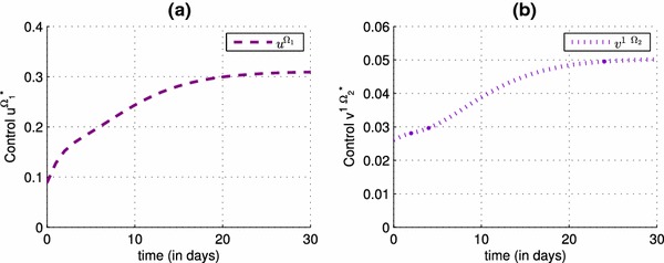
The optimal effectiveness of the vaccination control strategy: $u^{{\mathit{\Omega }}_1\ast }$ (see a), the optimal effectiveness of the travel-blocking control strategy: $v^{1{\mathit{\Omega }}_2}$ (see b)

Fig. 9.

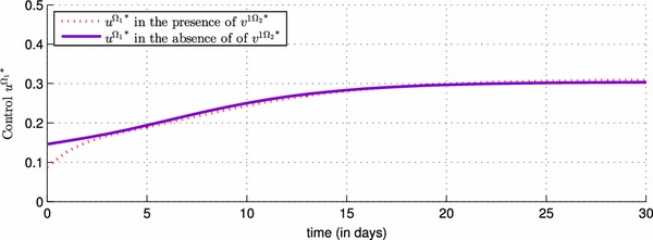
Comparison of control $u^{{\mathit{\Omega }}_1\ast }$ with and without use of control $v^{1{\mathit{\Omega }}_2}$

Fig. 10.

Comparison of control $u^{{\mathit{\Omega }}_1\ast }$ with and without use of control $v^{1{\mathit{\Omega }}_2}$ with different choices of $A_1$. a $u^{{\mathit{\Omega }}_1\ast }$ in the presence of control $v^{1{\mathit{\Omega }}_2}$. b $u^{{\mathit{\Omega }}_1\ast }$ in the absence of control $v^{1{\mathit{\Omega }}_2}$

Figure 11 also shows the impact of $A_1$ on the values of $v^{1{\mathit{\Omega }}_2}$, and we deduce that more $A_1$ is important, the more $v^{1{\mathit{\Omega }}_2}$ is also important. In fact, by analogous conclusions from Fig. 5, we deduce that in the case of a travel-blocking control that the more the control severity weight $A_1$ is big, the more the number of infected people in (a) is big, because $u^{{\mathit{\Omega }}_1}$ has obviously an impact on the values of the control $v^{1{\mathit{\Omega }}_2}$ (see simulation Fig. 11b) as we explained above (the more $u^{{\mathit{\Omega }}_1}$ is small the more $v^{1{\mathit{\Omega }}_2}$ is big), and also these results are obtained from the fact that the most important role of the travel-blocking control $v^{1{\mathit{\Omega }}_2}$ is to decrease the number of the infected people $I^{{\mathit{\Omega }}_1}$ without forgetting that the more $v^{1{\mathit{\Omega }}_2}$ is closer to zero, the more the number infected becomes insignificant. Opposite results are obtained in Fig. 12 by changing the values of the control severity weight $B_2$, and we obtain small $v^{1{\mathit{\Omega }}_2}$ (see simulation Fig. 12b) whenever $B_2$ is taken small values because $B_2$ has obviously an impact on the values of the control $v^{1{\mathit{\Omega }}_2}$ from the control characterization (25).

Fig. 11.

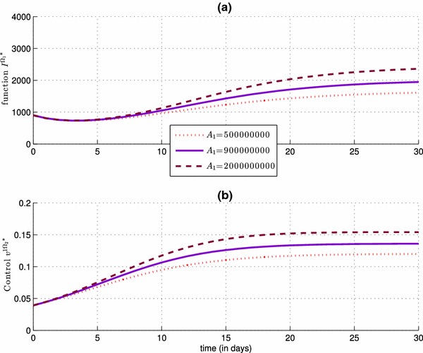
Impact of the control severity weight $A_1$, with $B_2=2.{10}^9$, on the number of the infected people in ${\mathit{\Omega }}_1$ (simulation a), and also on the control $v^{1{\mathit{\Omega }}_2}$ (simulation b)

Fig. 12.

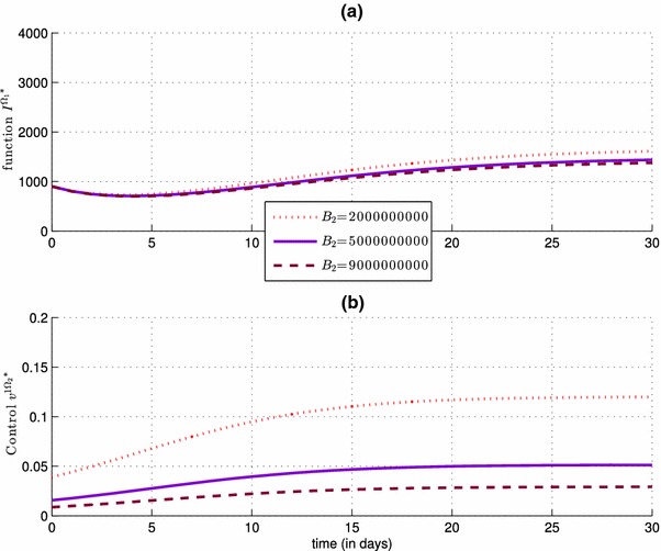
Impact of the control severity weight $B_2$, with $A_1=5.{10}^8$, on the number of the infected people in ${\mathit{\Omega }}_1$ (simulation a), and also on the control $v^{1{\mathit{\Omega }}_2}$ (simulation b)

For both Figs. 10 and 11, we can explain those numerical results by the fact that more $A_1$ is big, the more $u^{{\mathit{\Omega }}_1}$ is small (could obviously be deduced by the location of the severity weight $A_j$ in the denominator of the characterization formula (12) of $u^{{\mathit{\Omega }}_1}$ in Theorem 3.2.2, and then the effect of $v^{1{\mathit{\Omega }}_2}$ becomes important and valuable. We can obtain analogous results for $v^{1{\mathit{\Omega }}_2}$ when we change the values of the severity weight $B_2$ associated to the control $v^{1{\mathit{\Omega }}_2}$, as we see in Fig. 12.

Conclusion

We analyzed in this work two different optimal control problems for a discrete-time multi-regions SIR epidemic model. In the first part, only one control that characterizes the effectiveness of vaccination is used, and where the optimal control problem was subject of an optimization criterion represented by the minimization of an objective function aiming to minimize the number of infected people and the cost of vaccination while maximizing the number of removed people in the targeted region aiming to control. Numerical results, associated to this first part, showed the effectiveness of this vaccination while the targeted region was still sensitive to infection rates in its neighboring domains at high-risk. Then, we extended the first part to a second part by adding a travel-blocking control, in which we have controlled contacts between susceptible people of the controlled region (by vaccination) and the infected of domains at high-risk of infection. We showed the advantage of each case studied with a comparison between the numerical simulations they provided. We have identified optimal control strategies for several values of the controls severity weights to show the importance and the effectiveness of our approach in controlling the infection spread. Control programs that follow those strategies can effectively reduce the number of infected cases and increase the number of the removed individuals in a specific region.

References

- 1.Kermack WO, McKendrick AG (1927) Proc R Soc Edin A 115:700
- 2.Roberts M, Andreasen V, Lloyd A, Pillis L. Nine challenges for deterministic epidemic models. Epidemics. 2015;10:49–53. doi: 10.1016/j.epidem.2014.09.006. [DOI] [PMC free article] [PubMed] [Google Scholar]
- 3.Arino J, Jordan R, Van den Driessche P. Quarantine in a multi-species epidemic model with spatial dynamics. Math Biosci. 2007;206(1):46–60. doi: 10.1016/j.mbs.2005.09.002. [DOI] [PubMed] [Google Scholar]
- 4.Weiss RA. The Leeuwenhoek Lecture 2001. Animal origins of human infectious disease. Philos Trans R Soc B Biol Sci. 2001;356(1410):957–977. doi: 10.1098/rstb.2001.0838. [DOI] [PMC free article] [PubMed] [Google Scholar]
- 5.Baize S, Pannetier D, Oestereich L, Rieger T, Koivogui L, Magassouba N, et al. Emergence of Zaire Ebola virus disease in Guinea. N Engl J Med. 2014;371(15):1418–1425. doi: 10.1056/NEJMoa1404505. [DOI] [PubMed] [Google Scholar]
- 6.Arino J, Van Den Driessche P (2003) The basic reproduction number in a multi-city compartmental epidemic model. In: Positive systems. Springer, Berlin Heidelberg, pp 135–142
- 7.Arino J, Van den Driessche P. A multi-city epidemic model. Math Popul Stud. 2003;10(3):175–193. doi: 10.1080/08898480306720. [DOI] [Google Scholar]
- 8.Allen LJS, Jones MA, Martin CF. A discrete-time model with vaccination for a measles epidemic. Math Biosci. 1991;105(1):111–131. doi: 10.1016/0025-5564(91)90051-J. [DOI] [PubMed] [Google Scholar]
- 9.National portal of territorial collectivities (2015) (Portail national des collectivitées territoriales (P.N.C.L)). Ministry of interior-Morocco. http://www.pncl.gov.ma/fr/Pages/default.aspx
- 10.Longini IM. The generalized discrete-time epidemic model with immunity: a synthesis. Math Biosci. 1986;82(1):19–41. doi: 10.1016/0025-5564(86)90003-9. [DOI] [Google Scholar]
- 11.Allen LJ, Burgin AM. Comparison of deterministic and stochastic SIS and SIR models in discrete time. Math Biosci. 2000;163(1):1–33. doi: 10.1016/S0025-5564(99)00047-4. [DOI] [PubMed] [Google Scholar]
- 12.Allen LJ. Some discrete-time SI, SIR, and SIS epidemic models. Math Biosci. 1994;124(1):83–105. doi: 10.1016/0025-5564(94)90025-6. [DOI] [PubMed] [Google Scholar]
- 13.Brauera F, Fenga Z, Castillo-Chaveza C. Discrete epidemic models. Math Biosci. 2010;7:1. doi: 10.3934/mbe.2010.7.1. [DOI] [PubMed] [Google Scholar]
- 14.Enatsu Y, Nakata Y, Muroya Y. Global stability for a class of discrete SIR epidemic models. Math Biosci Eng. 2010;7(2):347–361. doi: 10.3934/mbe.2010.7.347. [DOI] [PubMed] [Google Scholar]
- 15.Ma X, Zhou Y, Cao H. Global stability of the endemic equilibrium of a discrete SIR epidemic model. Adv Differ Equ. 2013;2013(1):1–19. doi: 10.1186/1687-1847-2013-1. [DOI] [PMC free article] [PubMed] [Google Scholar]
- 16.Jung E, Lenhart S, Feng Z. Optimal control of treatments in a two-strain tuberculosis model. Discrete Contin Dyn Syst Ser B. 2002;2(4):473–482. doi: 10.3934/dcdsb.2002.2.473. [DOI] [Google Scholar]
- 17.Moualeu DP, Weiser M, Ehrig R, Deuflhard P. Optimal control for a tuberculosis model with undetected cases in Cameroon. Commun Nonlinear Sci Numer Simul. 2015;20(3):986–1003. doi: 10.1016/j.cnsns.2014.06.037. [DOI] [Google Scholar]
- 18.Silva CJ, Torres DFM. Optimal control for a tuberculosis model with reinfection and postexposure interventions. Math Biosci. 2013;244(2):154–164. doi: 10.1016/j.mbs.2013.05.005. [DOI] [PubMed] [Google Scholar]
- 19.Agusto FB, Adekunle AI. Optimal control of a two-strain tuberculosis-HIV/AIDS co-infection model. Biosystems. 2014;119:20–44. doi: 10.1016/j.biosystems.2014.03.006. [DOI] [PubMed] [Google Scholar]
- 20.Whang S, Choi S, Jung E. A dynamic model for tuberculosis transmission and optimal treatment strategies in South Korea. J Theor Biol. 2011;279(1):120–131. doi: 10.1016/j.jtbi.2011.03.009. [DOI] [PubMed] [Google Scholar]
- 21.Kim BN, Nah K, Chu C, Ryu SU, Kang YH, Kim Y. Optimal control strategy of Plasmodium vivax malaria transmission in Korea. Osong Public Health Res Perspect. 2012;3(3):128–136. doi: 10.1016/j.phrp.2012.07.005. [DOI] [PMC free article] [PubMed] [Google Scholar]
- 22.Prosper O, Ruktanonchai N, Martcheva M. Optimal vaccination and bednet maintenance for the control of malaria in a region with naturally acquired immunity. J Theor Biol. 2014;353:142–156. doi: 10.1016/j.jtbi.2014.03.013. [DOI] [PubMed] [Google Scholar]
- 23.Joshi HR. Optimal control of an HIV immunology model. Optim Control Appl Methods. 2002;23(4):199–213. doi: 10.1002/oca.710. [DOI] [Google Scholar]
- 24.Fister KR, Lenhart S, McNally JS. Optimizing chemotherapy in an HIV model. Electron J Differ Equ. 1998;1998(32):1–12. [Google Scholar]
- 25.Yang Y, Xiao Y, Wu J. Pulse HIV vaccination: feasibility for virus eradication and optimal vaccination schedule. Bull Math Biol. 2013;75:725–751. doi: 10.1007/s11538-013-9831-8. [DOI] [PubMed] [Google Scholar]
- 26.Kwon HD, Lee J, Yang SD. Optimal control of an age-structured model of HIV infection. Appl Math Comput. 2012;219(5):2766–2779. [Google Scholar]
- 27.Roshanfekr M, Farahi MH, Rahbarian R. A different approach of optimal control on an HIV immunology model. Ain Shams Eng J. 2014;5(1):213–219. doi: 10.1016/j.asej.2013.05.004. [DOI] [Google Scholar]
- 28.Zhou Y, Liang Y, Wu J. An optimal strategy for HIV multitherapy. J Comput Appl Math. 2014;263:326–337. doi: 10.1016/j.cam.2013.12.007. [DOI] [Google Scholar]
- 29.Adams BM, Banks HT, Davidian M, Kwon HD, Tran HT, Wynne SN, Rosenberg ES. HIV dynamics: modeling, data analysis, and optimal treatment protocols. J Comput Appl Math. 2005;184(1):10–49. doi: 10.1016/j.cam.2005.02.004. [DOI] [Google Scholar]
- 30.Costanza V, Rivadeneira PS, Biafore FL, D’Attellis CE. Optimizing thymic recovery in HIV patients through multidrug therapies. Biomed Signal Process Control. 2013;8(1):90–97. doi: 10.1016/j.bspc.2012.06.002. [DOI] [Google Scholar]
- 31.Zakary O, Rachik M, Elmouki I. On the impact of awareness programs in HIV/AIDS prevention: an SIR model with optimal control. Int J Comput Appl. 2016;133(9):1–6. [Google Scholar]
- 32.Chakrabarty SP, Joshi HR. Optimally controlled treatment strategy using interferon and ribavirin for hepatitis C. J Biol Syst. 2009;17(01):97–110. doi: 10.1142/S0218339009002727. [DOI] [Google Scholar]
- 33.Zakary O, Rachik M, Elmouki I. On effectiveness of an optimal antiviral bitherapy in HBV-HDV coinfection model. Int J Comput Appl. 2015;127(12):1–10. [Google Scholar]
- 34.Grsbll K, Ene C, Bdker R, Christiansen LE. Optimal vaccination strategies against vector-borne diseases. Spat Spatio Temp Epidemiol. 2014;11:153–162. doi: 10.1016/j.sste.2014.07.005. [DOI] [PubMed] [Google Scholar]
- 35.Burden TN, Ernstberger J, Fister KR. Optimal control applied to immunotherapy. Discrete Contin Dyn Syst Ser B. 2004;4(1):135–146. [Google Scholar]
- 36.Ledzewicz U, Schättler H. Antiangiogenic therapy in cancer treatment as an optimal control problem. SIAM J Control Optim. 2007;46(3):1052–1079. doi: 10.1137/060665294. [DOI] [Google Scholar]
- 37.Castiglione F, Piccoli B. Cancer immunotherapy, mathematical modeling and optimal control. J Theor Biol. 2007;247(4):723–732. doi: 10.1016/j.jtbi.2007.04.003. [DOI] [PubMed] [Google Scholar]
- 38.Elmouki I, Saadi S. Quadratic and linear controls developing an optimal treatment for the use of BCG immunotherapy in superficial bladder cancer. Optim Control Appl Methods. 2015;37(1):176–189. doi: 10.1002/oca.2161. [DOI] [Google Scholar]
- 39.Martin RB. Optimal control drug scheduling of cancer chemotherapy. Automatica. 1992;28(6):1113–1123. doi: 10.1016/0005-1098(92)90054-J. [DOI] [Google Scholar]
- 40.Engelhart M, Lebiedz D, Sager S. Optimal control for selected cancer chemotherapy ODE models: a view on the potential of optimal schedules and choice of objective function. Math Biosci. 2011;229(1):123–134. doi: 10.1016/j.mbs.2010.11.007. [DOI] [PubMed] [Google Scholar]
- 41.Yan X, Zou Y. Optimal and sub-optimal quarantine and isolation control in SARS epidemics. Math Comput Model. 2008;47(1):235–245. doi: 10.1016/j.mcm.2007.04.003. [DOI] [PMC free article] [PubMed] [Google Scholar]
- 42.Agusto FB. Optimal isolation control strategies and cost-effectiveness analysis of a two-strain avian influenza model. Biosystems. 2013;113(3):155–164. doi: 10.1016/j.biosystems.2013.06.004. [DOI] [PubMed] [Google Scholar]
- 43.Brown VL, White KJ. The role of optimal control in assessing the most cost-effective implementation of a vaccination programme: HPV as a case study. Math Biosci. 2011;231(2):126–134. doi: 10.1016/j.mbs.2011.02.009. [DOI] [PubMed] [Google Scholar]
- 44.Su Y, Sun D (2015) Optimal control of anti-hbv treatment based on combination of traditional chinese medicine and western medicine. Biomed Signal Process Control 15:41–48
- 45.Buonomo B, Lacitignola D, Vargas-De-Len C. Qualitative analysis and optimal control of an epidemic model with vaccination and treatment. Math Comput Simul. 2014;100:88–102. doi: 10.1016/j.matcom.2013.11.005. [DOI] [Google Scholar]
- 46.Lowden J, Neilan RM, Yahdi M. Optimal control of vancomycin-resistant enterococci using preventive care and treatment of infections. Math Biosci. 2014;249:8–17. doi: 10.1016/j.mbs.2014.01.004. [DOI] [PubMed] [Google Scholar]
- 47.Apreutesei N, Dimitriu G, Strugariu R (2014) An optimal control problem for a two-prey and one-predator model with diffusion. Comput Math Appl 67(12):2127–2143
- 48.Dabbs K (2010) Optimal control in discrete pest control models. University of Tennessee Honors Thesis Projects
- 49.Pontryagin LS, Boltyanskii VG, Gamkrelidze RV, Mishchenko E. The mathematical theory of optimal processes (International series of monographs in pure and applied mathematics) New York: Interscience; 1962. [Google Scholar]