High-resolution 3D MR Fingerprinting using parallel imaging and deep learning

Abstract

MR Fingerprinting (MRF) is a relatively new imaging framework capable of providing accurate and simultaneous quantification of multiple tissue properties for improved tissue characterization and disease diagnosis. While 2D MRF has been widely available, extending the method to 3D MRF has been an actively pursued area of research as a 3D approach can provide a higher spatial resolution and better tissue characterization with an inherently higher signal-to-noise ratio. However, 3D MRF with a high spatial resolution requires lengthy acquisition times, especially for a large volume, making it impractical for most clinical applications. In this study, a high-resolution 3D MR Fingerprinting technique, combining parallel imaging and deep learning, was developed for rapid and simultaneous quantification of T₁ and T₂ relaxation times. Parallel imaging was first applied along the partition-encoding direction to reduce the amount of acquired data. An advanced convolutional neural network was then integrated with the MRF framework to extract features from the MRF signal evolution for improved tissue characterization and accelerated mapping. A modified 3D-MRF sequence was also developed in the study to acquire data to train the deep learning model that can be directly applied to prospectively accelerate 3D MRF scans. Our results of quantitative T₁ and T₂ maps demonstrate that improved tissue characterization can be achieved using the proposed method as compared to prior methods. With the integration of parallel imaging and deep learning techniques, whole-brain (26 × 26 × 18 cm³) quantitative T₁ and T₂ mapping with 1-mm isotropic resolution were achieved in ~7 min. In addition, a ~7-fold improvement in processing time to extract tissue properties was also accomplished with the deep learning approach as compared to the standard template matching method. All of these improvements make high-resolution whole-brain quantitative MR imaging feasible for clinical applications.

1. Introduction

MR Fingerprinting (MRF) is a relatively new imaging framework for MR acquisition, reconstruction, and analysis, which can provide rapid, efficient and simultaneous quantification of multiple tissue properties from a single acquisition (Ma et al., 2013). Compared to conventional MR imaging approaches, MRF uses pseudorandomized acquisition parameters (such as flip angles and repetition times) to generate unique signal signatures for different tissue types and retrieve quantitative tissue parameters using a template matching algorithm. Since its introduction in 2013, this technique has been successfully applied for quantitative imaging of multiple human organs including the brain, abdominal organs, heart, and breast (Badve et al., 2017; Chen et al., 2016, 2019b; Hamilton et al., 2017; Yu et al., 2017). The quantitative tissue properties obtained using MRF, such as T₁ and T₂ relaxation times, have been demonstrated to provide new insights into improved tissue characterization and disease diagnosis (Badve et al., 2017; Ma et al., 2019). Specifically for brain imaging, MRF has been applied for longitudinal characterization of brain development in early childhood, differentiation of brain tumor types, and improved detection and diagnosis of epileptic lesions (Badve et al., 2017; Chen et al., 2019a; Körzdörfer et al., 2019; Liao et al., 2018; Ma et al., 2019).

While previous studies have paved the way for clinical applications of MRF, to broadly adapt MRF into clinical examinations, MRF must meet several prerequisites, including whole-organ coverage, a sufficiently high resolution and a reasonable data acquisition time. To this end, significant efforts have been made to extend the original 2D MRF approaches to 3D imaging (Chen et al., 2019b; Liao et al., 2017; Ma et al., 2018). The extension to 3D MRF can potentially provide a higher spatial resolution and better tissue characterization with an inherently higher signal-to-noise ratio, which is favorable for pediatric neuroimaging and clinical diagnosis of small lesions in the brain. For 2D MRF acquisitions, thousands of MRF time frames are typically acquired for tissue characterization and each time frame/image is acquired with only one spiral interleaf, which is highly undersampled (Jiang et al., 2015; Ma et al., 2013). To maintain the high scan efficiency in 3D MRF, only one spiral arm is acquired for each partition in a 3D image and the same spiral arm is acquired along the partition direction within the volume (Ma et al., 2018). While MRF has demonstrated high efficiency compared to conventional quantitative imaging approaches, 3D MRF with a high spatial resolution still requires lengthy acquisition times, especially for whole-brain coverage, making it impractical for clinical applications. Therefore, multiple algorithms have been developed for accelerated 3D MRF acquisitions (see supplemental materials) (Liao et al., 2017; Ma et al., 2018). Since MRF is already highly undersampled in-plane with only one spiral readout, current approaches to accelerate 3D MRF have been focused on 1) acceleration along the partition direction and 2) reduction of MRF time frames for tissue characterization (Liao et al., 2017; Ma et al., 2018). One recent study utilized an interleaved sampling pattern along the partition-encoding direction to uniformly undersample the MRF dataset. With a reduction factor of 3, whole-brain coverage (~14 cm volume) was achieved with a spatial resolution of 1.2 × 1.2 × 3 mm³ in less than 5 min (Ma et al., 2018). Cartesian GRAPPA combined with sliding window reconstruction has also been developed to reconstruct uniformly undersampled 3D MRF datasets. Liao et al. demonstrated an improved accuracy as compared to the aforementioned interleaved sampling approach and a whole-brain scan (~19 cm volume) with a spatial resolution of 1.2 × 1.2 × 2 mm³ was achieved in ~3.5min (Liao et al., 2017). Acceleration of 3D MRF with higher spatial resolutions (1 mm³ or better) poses more technical challenges due to reduced SNR and has not been extensively explored and validated.

One important feature of MRF compared to most other quantitative MRI methods is the utilization of template matching for tissue characterization (Ma et al., 2013). However, this approach is relatively slow and requires a large amount of memory to store both the image dataset and the MRF dictionary (McGivney et al., 2014). More importantly, it relies on a comparison of global appearances of signal evolution from each pixel and hence does not take full advantage of the useful information acquired in MRF. Consequently, more than 1000 time points are typically required for accurate tissue characterization using template matching, which prolongs the MRF acquisition (Pierre et al., 2016). Advanced post-processing methods, capable of extracting valuable information in local regions of each signal evolution and measuring from neighboring pixels, can largely improve the performance of MRF in post-processing and therefore, reduce scan time.

Deep learning is an ideal solution for information retrieval from MRF measurements. Recent developments in machine learning have indicated that it is possible to accelerate 2D MRF acquisition using deep learning neural networks (Cohen et al., 2018; Fang et al., 2019; Hoppe et al., 2018, 2017). For example, Cohen et al. have developed a 4-layer neural network to extract tissue properties from a fully-sampled MRF dataset and the results demonstrated a 300–5000 fold improvement in processing speed (Cohen et al., 2018). Hoppe et al. have developed a convolutional neural network to exploit the correlation in the temporal domain and their results demonstrated that accurate tissue mapping can be achieved from MRF images with undersampled aliasing artifacts (Hoppe et al., 2018, 2017). To further utilize correlated information in the spatial domain, Fang et al. proposed a deep learning model with two modules, a feature extraction module and a spatially-constrained quantification module to improve the performance of tissue characterization. Instead of relying on information from a single pixel, a patch of 64 × 64 pixels was used as an input for the convolutional neural network (CNN) training and experimental results with a highly undersampled dataset demonstrated that accurate T₁ and T₂ quantification can be achieved with an up to 8-fold acceleration in the scan time (Fang et al., 2019). This suggests that more advanced features from MRF measurements can be extracted using the CNN network. Currently, these methods are applied with 2D MRF approaches and their utility for 3D MRF remains to be investigated. Compared to 2D MRF, the application of deep learning for 3D MRF faces more technical challenges to acquire the training dataset for the CNN model. The appropriate training dataset needs to provide 1) CNN model input, containing MRF signal evolutions with a reduced number of time frames, which mimic the real accelerated scans, and 2) ground-truth tissue property maps with decent image quality and no relative motion in regard to the input MRF signal. While retrospectively data undersampling can be used to achieve this goal for 2D MRF (Fang et al., 2019), this approach is not generally applicable for 3D MRF acquisitions.

This study aimed to combine state-of-the-art parallel imaging and deep learning techniques to develop a rapid 3D MRF method capable of achieving 1-mm isotropic resolution and whole brain coverage within a clinically feasible time window. A new 3D MRF sequence specifically designed to acquire the training dataset for 3D acquisitions was developed. Our results demonstrate that the trained CNN model can be applied to acquire high-resolution T₁ and T₂ maps from prospectively accelerated 3D MRF acquisitions.

2. Materials and methods

2.1. 3D MRF for brain imaging

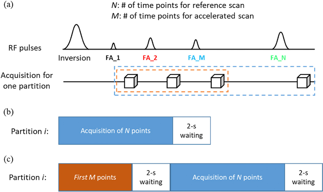
All MRI experiments in this study were performed on a Siemens 3T Prisma scanner with a 32-channel head coil. A 3D MRF sequence based on the steady-state free precession (SSFP) readout was used for volumetric brain MRF with 1-mm isotropic resolution (Chen et al., 2019b). Compared to the original 2D MRF method, a linear slice-encoding gradient was applied for volumetric encoding and the 3D MRF dataset was acquired sequentially through partitions. The data acquisition for each partition was performed with pseudorandomized flip angles and a highly-undersampled spiral readout, which is similar to the standard 2D MRF (Fig. 1a). The same acquisition parameters, such as the flip angle pattern and in-plane spiral readouts, were repeated for each partition in the 3D sampling scan and a constant waiting time of 2 s was applied between partitions for longitudinal recovery (Fig. 1b). Other imaging parameters included: FOV, 25 cm; matrix size, 256; TR, 9.1 ms; TE, 1.3 ms; flip angle range, [5°, 12°]. A total of 768 time frames were acquired to generate MRF signal evolution and the acquisition time including the 2-sec waiting time was ~17 s per partition.

Fig. 1.

Diagram of 3D MRF sequences. (a) Similar to the standard 2D MRF sequence, pseudorandom acquisition parameters, such as the flip angles (FA), were applied in the 3D MRF acquisition. (b) Standard 3D MRF sequence (3DMRF-S) with N time frames. A 2-sec waiting time was applied after data acquisition of each partition for partial longitudinal relaxation. (c) Modified 3D MRF sequence for acquiring training dataset for deep learning (3DMRF-DL). An extra section containing the pulse sequence for the first M time points was added at the beginning of the acquisition for each partition to simulate the spin history of the accelerated scan.

Similar to the standard MRF method, the acquired MRF signal evolution from each voxel was matched to a pre-defined MRF dictionary to extract quantitative T₁ and T₂ relaxation times (Ma et al., 2013). The MRF dictionary was generated using Bloch equation simulations with the actual acquisition parameters. A total of ~23,000 entries are contained in the MRF dictionary, which covers a wide range of T₁ (60–5000 ms) and T₂ (10–500 ms) values. The step sizes of T₁ in the dictionary were 10 ms between 60 and 2000 ms, 20 ms between 2000 and 3000 ms, 50 ms between 3000 and 3500 ms, and 500 ms between 4000 and 5000 ms. The step sizes of T₂ were 2 ms between 10 and 100 ms, 5 ms between 100 and 200 ms, and 10 ms between 200 and 500 ms.

2.2. Acceleration of 3D MRF with parallel imaging

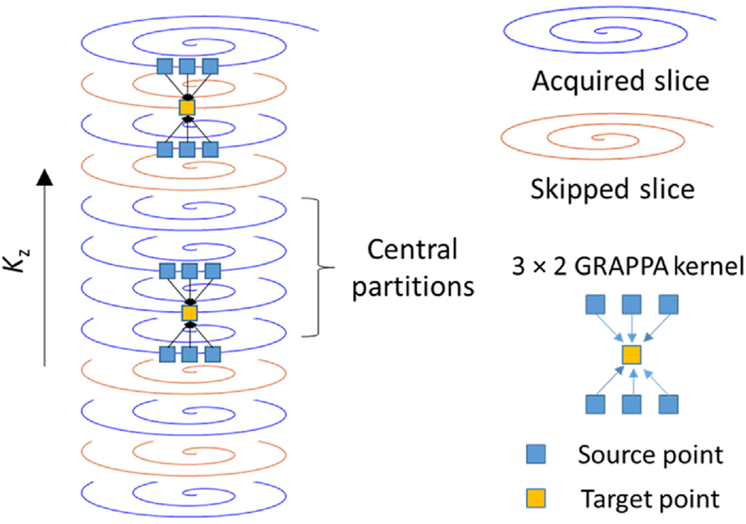
In this study, parallel imaging along the partition-encoding direction was applied to accelerate the 3D MRF acquisition. An interleaved sampling pattern introduced by (Ma et al., 2018) was used to undersample data in the partition direction. Parallel imaging reconstruction, similar to the through-time spiral GRAPPA technique, was applied to reconstruct the missing k-space points with a 3 × 2 GRAPPA kernel along the spiral readout × partition-encoding direction (Fig. 2). The calibration data for the GRAPPA weight were obtained from the center k-space in the partition direction and integrated into the final image reconstruction for preserved tissue contrast. One challenge for parallel imaging reconstruction with non-Cartesian trajectories, such as the spiral readout used in MRF acquisition, was to obtain sufficient repetition of the GRAPPA kernels for robust estimation of GRAPPA weights. Similar to the approach for the spiral GRAPPA technique (Chen et al., 2015; Seiberlich et al., 2011), eight GRAPPA kernels with a similar shape and orientation along the spiral readout direction were used in this study to increase the number of kernel repetitions. After GRAPPA reconstruction, each MRF time point/volume still had one spiral arm in-plane, but all missing spiral arms along the partition direction were filled as illustrated in Fig. 2.

Fig. 2.

GRAPPA reconstruction along the partition-encoding direction. A 3 × 2 GRAPPA kernel was used to fill the missing k-space points. The GRAPPA weights were calibrated using the calibration data acquired from the central partitions. Since the kernel size and orientation vary along the spiral readout (Chen et al., 2015; Seiberlich et al., 2011), this reconstruction process was repeated for all the points along the spiral interleaves.

2.3. Convolutional neural network

Aside from acceleration using parallel imaging, we further leveraged the deep learning method to reduce acquisition time by extracting features in the acquired MRF dataset that are needed for accurate tissue characterization. To describe the workflow of the 3D MRF, we will first briefly review how deep learning has been integrated into a 2D MRF framework. As introduced by Fang et al. (2019), the ground truth tissue property maps (T₁ and T₂) were obtained using the template matching algorithm from a MRF dataset consisting of N time frames (Fig. 1a). One way to accelerate MRF with deep learning is to achieve a similar tissue map quality with only the first M time points (M < N). To train the CNN model, the MRF signal evolution from M time points was used as the input of the CNN network and the desired output was set as the ground truth tissue maps obtained from all N points. To ensure data consistency and minimize the potential motion between the network input and output, the input data of M points was generally obtained from retrospective undersampling of the reference data with all N points. For 2D measurements, given a certain delay time (5–10 s) generally exists between scans for system adjustments and other purposes, it is reasonable to assume that brain tissues reach a fully longitudinally recovered state and each acquisition starts from a longitudinal magnetization (M_z) of 1. Therefore, the retrospectively undersampled MRF data and the data from prospectively accelerated cases should have the same signal evolution for the same tissues, independent of the spin history from the previous scan. The CNN parameters determined in this manner can be directly applied to extract tissue properties from the prospectively acquired dataset.

While a similar method as outlined above for 2D can potentially be applied to reduce data sampling and accelerate 3D MRF, important modifications are required due to the additional partition encoding. For a 3D MRF acquisition, a short waiting time (2 s in this study) was applied between partitions (Fig. 1), which is insufficient for most brain tissues to achieve full recovery of longitudinal magnetization. As a result, the magnetization at the beginning of each partition acquisition depends on the settings used in acquiring the previous partition, including the number of MRF time frames. Under this circumstance, the retrospectively shortened signal evolution with M time points (from a total of N time points) does not agree with the signal from prospectively accelerated scans (see Fig. S1). Consequently, the CNN model trained using the aforementioned 2D approach is not applicable for the prospectively accelerated data. In order to train a CNN model for prospectively accelerated 3D MRF data, a new 3D MRF sequence was developed in this study.

The new pulse sequence had a similar sequence structure as the standard 3D MRF with the exception that an extra section was inserted to mimic the condition of the prospectively accelerated MRF acquisition (Fig. 1c). This additional section consisted of a pulse sequence section for data sampling of the first M time points followed by a 2-sec waiting time. The purpose of this additional section was to ensure the same magnetization history as that in a real accelerated case so that the first M time points acquired in the second section (the whole section contains N time points) matched with the data in the actual accelerated scan (Fig. S1). With this modification, the MRF data obtained in the second section of the new sequence can 1) provide reference T₁ and T₂ maps as the ground truth for CNN training using all N time points and 2) generate retrospectively shortened MRF data (with the first M time points) as the input for training. Since the purpose of the additional section was to create a magnetization history, no data acquisition was needed for this section. Here, we named the new 3D MRF sequence for deep learning as 3DMRF-DL and the standard sequence without the additional section as 3DMRF-S.

Before the application of the developed 3DMRF-DL method for in vivo measurements, phantom experiments were performed using a phantom with M_nCl₂ doped water to evaluate its quantitative accuracy. T₁ and T₂ values obtained using 3DMRF-DL were compared to those obtained with the reference methods using single-echo spin-echo sequences and the 3DMRF-S method. Both the 3DMRF-DL and 3DMRF-S methods were conducted with 1-mm isotropic resolution and 48 partitions. The reference method with spin-echo sequences was acquired from a single slice with a FOV of 25 cm and a matrix size of 128.

To use the 3DMRF-DL method to establish CNN for prospectively accelerated 3D MRF scans, the optimal number of time points (M) needs to be determined. A testing dataset from five normal subjects (M:F, 2:3; mean age, 35 ± 10 years) using the 3DMRF-S method was acquired for this purpose. Informed consent was obtained from all the subjects before the experiments. The 3DMRF-S scan was performed with 1-mm resolution covering 96 partitions and 768 time points. Reference T₁ and T₂ maps were obtained with the template matching method and used as the ground truth for the CNN network. To identify the optimal number of time frames, the CNN model was trained with various M values (96, 144, 192 and 288) using retrospective undersampling. Since the determination of optimal time frame is also coupled with the settings of parallel imaging, the extracted input data was also retrospectively undersampled along the partition direction with reduction factors of 2 or 3 and then reconstructed with parallel imaging. MRF data containing nearly 400 input datasets from four subjects (96 partitions for each subject) was used for network training and the data from the remaining subject was used for validation. The validation dataset was applied to evaluate the performance of the model after the network training was completed. This information was not utilized to fine-tune the model during the training process. T₁ and T₂ maps obtained from various time points and reduction factors were compared to the ground truth maps and normalized root-mean-square-error (NRMSE) values were calculated to evaluate the performance and identify the optimal time point for the 3DMRF-DL method. A leave-one-subject-out cross validation was performed across all five subjects. One thing to note is that the CNN model training in this step cannot be applied to prospective accelerated data as discussed previously.

Similar to the approach proposed by Fang et al. (2019), a CNN model with two major modules, a feature extraction module and a U-Net module, was used in the current study (Fig. 3). To train the CNN, image patches of size 64 × 64 were extracted from the MRF dataset with a stride of 32 and used as the training samples. The loss function for training was defined as the relative difference between estimated tissue property value ( $\hat{\theta }$ ) and the ground truth value (θ), i.e., Loss = ${\mathbb{E}}_{\hat{\theta },\theta }|(\hat{\theta }-\theta )/\theta |$ . The CNN parameters were initialized from a Gaussian distribution with zero mean and standard deviation of 0.02. Adam optimizer was used with a batch size of 32 and an initial learning rate of 0.0002. The CNN was trained for a total of 400 epochs, with the learning rate remained unchanged for the first 200 epochs and linearly decayed to zero in the next 200 epochs. The algorithm was implemented in Python using the PyTorch library and the whole training took around three days using an NVIDIA GeForce GTX TITAN XP GPU.

Fig. 3.

Schematic overview of the CNN model with two modules for tissue property mapping. The feature extraction module (FE) consists of four fully-connected layers (FNN), which is designed to mimic singular value decomposition to reduce the dimension of signal evolutions (McGivney et al., 2014). The U-Net structure was used for the spatially-constrained quantification (SQ) module to capture spatial information from neighboring pixels for improved quantification of tissue properties. MRF images of 3 contiguous slices (red) were used as input, and the corresponding reference T₁ and T₂ maps from the central slice were used as output for the network.

2.4. In vivo experiments with 3DMRF-DL

After the determination of the optimal number of time points (M) for the accelerated scans, in vivo experiments were performed on a separate group of subjects including seven normal volunteers (M:F, 4:3; mean age, 36 ± 10 years) to evaluate the proposed method using parallel imaging and deep learning. For each subject, two separate scans were performed. The first scan was acquired using the 3DMRF-DL sequence with 144 slices. A total of 768 time points was acquired and no data undersampling was applied along the partition direction. For the second scan, the 3DMRF-S sequence was used with prospective data undersampling, which includes sampling with a reduced number of time points (M) and acceleration along the partition direction. Whole brain coverage (160–176 sagittal slices) was achieved for all subjects. CNN model was then trained using the same approach outlined above using the data acquired with the 3DMRF-DL sequence. This trained model can be directly applied to extract T₁ and T₂ maps from the second prospectively accelerated scan using the 3DMRF-S sequence. A leave-one-subject-out cross-validation was used to obtain T₁ and T₂ values from all seven subjects, namely no data from the same subject was used for the training and validation simultaneously.

After tissue quantification using CNN, brain segmentation was further performed on both datasets to enable comparison of T₁ and T₂ values obtained from the two separate scans. Specifically, T₁-weighted MPRAGE images were first synthesized based on the quantitative tissue maps (Deichmann et al., 2000). These MPRAGE images were used as the input and subsequent brain segmentation was performed using the Freesurfer software (Fischl et al., 2002). Based on the segmentation results, mean T₁ and T₂ values from multiple brain regions, including white matter, cortical gray matter and subcortical gray matter, were extracted from each subject and the results were compared between the two MRF scans.

The T₁ and T₂ quantification with the proposed method was further validated with standard relaxometry methods. The prospectively undersampling 3DMRF-S method with 192 time points was acquired on one subject and T₁ and T₂ maps with whole-brain coverage were extracted using the CNN network. A standard 2D inversion-recovery sequence with eight inversion times (240, 480, 720, 1000, 1500, 2000, 2500, and 3000 ms) was applied to obtain the T₁ maps from the same subject. The T₂ values were obtained using a standard 2D single-echo spin-echo sequence with six TE values (10, 30, 50, 100, 150 and 200 ms). For the standard methods, the in-plane resolution was 1 mm (FOV, 25 cm; matrix size, 256) and slice thickness was 5 mm.

3. Results

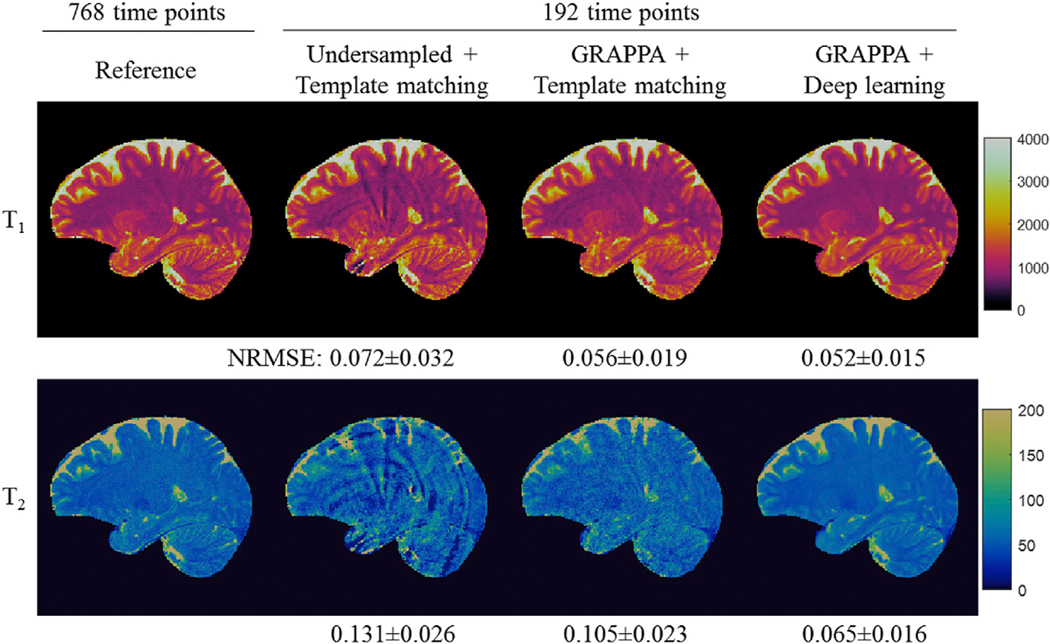
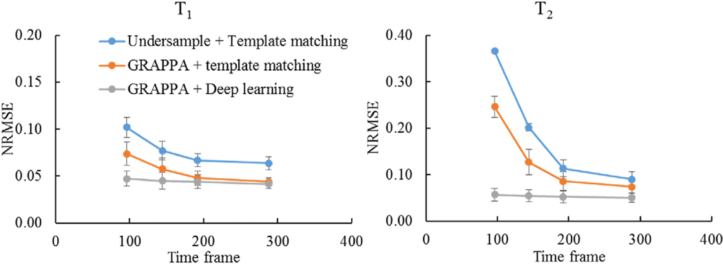
The 3DMRF-S sequence (Fig. 1b) was first applied to identify the optimal number of MRF time points and parallel imaging settings along the partition direction. MRF measurements from five subjects were retrospectively undersampled and reconstructed using parallel imaging and deep learning modeling. The results were further compared to those obtained using template matching alone or template matching after GRAPPA reconstruction. Fig. 4 shows representative results obtained from 192 time frames with an acceleration factor of 2 in the partition-encoding direction. With 1-mm isotropic resolution, significant residual artifacts were noticed in both T₁ and T₂ maps processed with the template matching alone. With the GRAPPA reconstruction, most of the artifacts in T₁ maps were eliminated, but some residual artifacts were still noticeable in T₂ maps. Comparing the two approaches, the quantitative maps obtained with the proposed method with both GRAPPA reconstruction and deep learning modeling presented a similar quality to the reference maps. The lowest NRMSE values were obtained with the proposed method among all three methods. These findings are consistent for all other numbers of time points tested, ranging from 96 (12.5% of the total number of points acquired) to 288 (37.5%) as shown in Fig. 5.

Fig. 4.

Representative T₁ and T₂ maps obtained from retrospectively undersampled 3D MRF dataset acquired using the 3DMRF-S sequence. The results were obtained using the first 192 time points with a reduction factor of 2 along the partition-encoding direction (R = 2). NRMSE values were calculated as compared to the reference maps. The mean and standard deviation values obtained from all the slices acquired from the subject are presented in the figure. Lower NRMSE values were observed for both T₁ and T₂ quantification with the proposed method as compared to the previous methods, such as the interleaved sampling method (Undersampled + Template matching) or parallel imaging method (GRAPPA + Template matching).

Fig. 5.

Comparison of NRMSE values for T₁ and T₂ quantification between three different post-processing methods, including the interleaved sampling method (Undersampled + Template matching), parallel imaging method (GRAPPA + Template matching), and the proposed method (GRAPPA + Deep learning). The results were obtained from a retrospectively undersampled 3D MRF dataset acquired using the standard 3D MRF sequence (R = 2). The proposed method demonstrates better performance, especially with highly reduced data sampling. The error bar represents the standard deviation of NRMSE values obtained from the leave-one-subject-out cross validation.

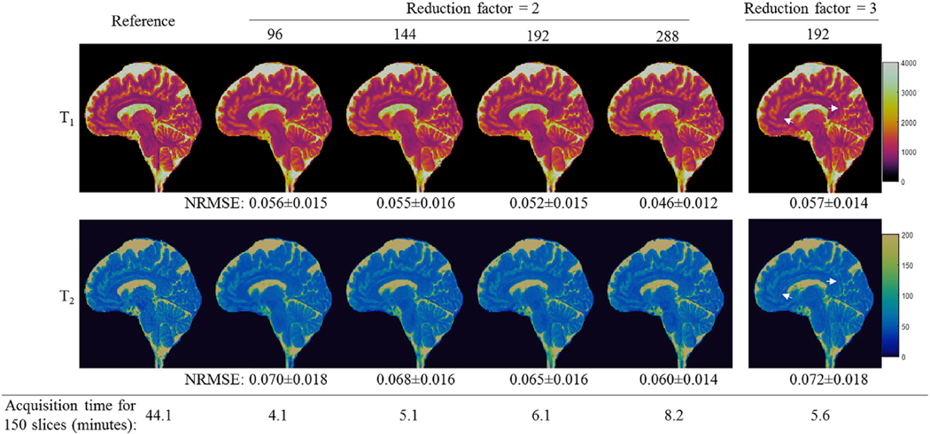
Fig. 6 shows representative T₁ and T₂ maps obtained using the 3DMRF-S method and different numbers of time points. With an acceleration factor of 2 along the partition encoding direction, high quality quantitative maps with 1-mm isotropic resolution were obtained for all cases. When the number of time points increased, NRMSE values decreased for both T₁ and T₂ maps. However, this improvement in tissue quantification was achieved at a cost of more sampling data and thus longer acquisition times. With the current design of the 3DMRF-S sequence (R = 2), the sampling time for 150 slices (15-cm coverage) was increased from 4.1 min to 8.2 min when the number of time frames increased from 96 to 288. Compared to the case with a reduction factor of 2, some residual aliasing artifacts were noted in the quantitative maps obtained with a reduction factor of 3 (Fig. 6). A leave-one-subject-out cross validation was performed for this experiment and consistent findings were achieved across all five tested subjects. In order to balance the image quality and scan time, a reduction factor of 2 with 192 time points was selected as the optimal setting for in vivo testing using the 3DMRF-DL approach.

Fig. 6.

Representative T₁ and T₂ maps obtained using the 3DMRF-S method and different MRF time frames ranging from 96 (12.5%) to 288 (37.5%). High-quality tissue quantitative maps with 1-mm isotropic resolution were obtained for all the cases. The corresponding acquisition time for each sampling pattern is also presented. One case with a reduction factor of 3 is shown (right-most column), and some residual artifacts were noticed with this case with a higher reduction factor. NRMSE values were calculate from all the slices acquired for this subject. The mean and standard deviation values are presented in the figure.

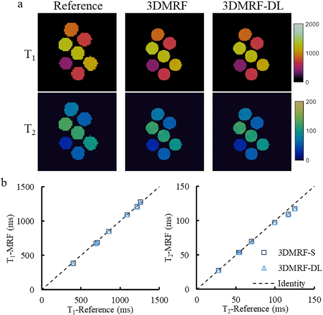
Before the application of the 3DMRF-DL sequence for in vivo measurements, its accuracy in T₁ and T₂ quantification was first evaluated using phantom experiments and the results are shown in Fig. 7. A total of 768 time points were acquired for both the 3DMRF-DL and 3DMRF-S sequences. For the 3DMRF-DL method, the first section contains 192 time points as determined in previous experiments. The T₁ and T₂ values obtained using the 3DMRF-DL method were consistent with the reference values for a wide range of T₁ [400–1300 ms] and T₂ [30 and 130 ms] values. The average percent errors over all seven vials in the phantom were 1.7 ± 2.2% and 1.3 ± 2.9% for T₁ and T₂, respectively. The quality of the quantitative maps also matches the results acquired using the 3DMRF-S sequence. The NRMSE value was 0.062 for T₁ and 0.046 for T₂ between the results from the two 3D MRF approaches.

Fig. 7.

Phantom measurements. (a) Representative T₁ and T₂ maps obtained using the 3DMRF-S and 3DMRF-DL sequences as compared to the results from the reference scans. (b) Comparison of quantitative T₁ and T₂ values between the reference and the two 3D MRF methods.

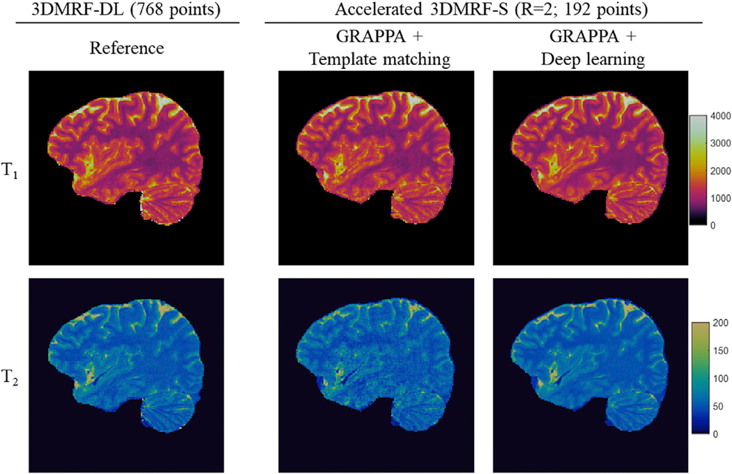
Based on the optimal time points (M, 192 points) and undersampling patterns (R = 2), the 3DMRF-DL method was used to establish a CNN network for prospectively accelerated 3D MRF data. The experiments were performed on seven subjects. Two MRF scans were acquired for each subject, including one with all 768 time points using the 3DMRF-DL sequence and the other with only 192 points and prospectively accelerated 3DMRF-S sequence. With the latter approach, about 160–176 slices were acquired for each subject to achieve whole-brain coverage and the acquisition time varied between 6.5 min and 7.1 min. Leave-one-subject-out cross validation was performed to extract quantitative T₁ and T₂ values for all subjects and the quantitative maps from both scans were calculated. Representative T₁ and T₂ maps obtained from the prospectively accelerated scan (3DMRF-S) are presented in Fig. 8. Some residual artifacts were noted in the images acquired with the GRAPPA + template matching approach but were minimized using the proposed method - combining GRAPPA with deep learning. The quantitative maps obtained from a similar slice location using the 3DMRF-DL method (served as the reference maps with all 768 time points) were also plotted for comparison (left column in Fig. 8). While subjects could have moved between the two separate scans, a good agreement was found between both brain anatomy and image quality.

Fig. 8.

Representative T₁ and T₂ maps obtained using the prospectively accelerated scans (3DMRF-S) with R = 2 and 192 points. The results obtained using the 3DMRF-DL method with all 768 time points from the same subject at a similar slice location are also shown as a comparison (left column). Improved map quality was achieved with the proposed method using GRAPPA and deep learning (right-most column) as compared to the previous method using GRAPPA and template matching (middle column).

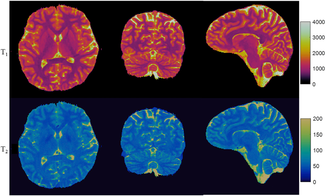
Representative T₁ and T₂ maps obtained using the accelerated scans from three different views are shown in Fig. 9. The results further demonstrate that high-quality 3D MRF with 1-mm resolution and whole-brain coverage can be achieved with the proposed approach in about 7 min. In addition, the time to extract tissue properties was also largely reduced to 2.5 s/slice using the CNN method, which represents a 7-fold of improvement compared to the template matching method (~18 s/slice). While all processing times were calculated based on computations performed on a CPU, further acceleration in processing time can be achieved with direct implementation on a GPU card (0.02 s/slice).

Fig. 9.

Reformatted quantitative maps in axial, coronal and sagittal views from the prospectively accelerated scan (3DMRF-S; R = 2; 192 time points). The acquisition time for 176 slices was about 7 min.

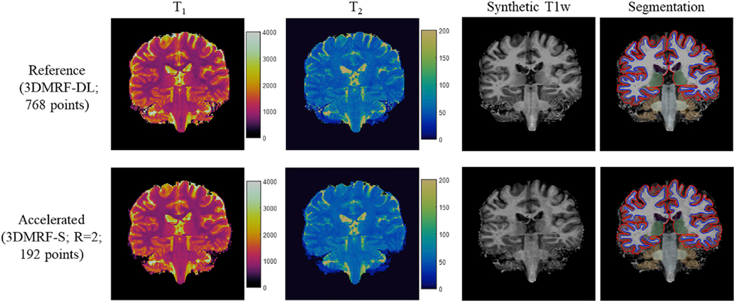
Representative segmentation results based on the MRF measurements are presented in Fig. 10. The quantitative T₁ and T₂ maps obtained using both the 3DMRF-DL sequence and the prospectively accelerated 3DMRF sequence are plotted, along with the synthetic T₁-weighted MPRAGE images and brain segmentation results. Different brain regions, such as white matter, gray matter, and the thalamus, are illustrated with different colors in the maps and the segmentation results matched well between the two MRF scans. Based on the brain segmentation results, quantitative T₁ and T₂ values from multiple brain regions are summarized in Table 1. Compared to the reference values obtained using the 3DMRF-DL sequence with 768 time points, accurate tissue parameter quantification was achieved with the proposed rapid 3D MRF method and the mean percentage error was 1.0 ± 0.7% and 1.9 ± 0.7% for T₁ and T₂, respectively.

Fig. 10.

Representative brain segmentation results from MRF measurements. Synthetic T1-weighted images were generated based on quantitative MRF measurements and used as the input for image segmentation using Freesurfer. Results from both the 3DMRF-DL method and prospectively accelerated scan (3DMRF-S) from the same subject at a similar slice location are presented. Quantitative T₁ and T₂ values from multiple brain regions were extracted from both scans based on the segmentation results.

Table 1.

Summary of T₁ and T₂ relaxation times from different brain regions. Results from both the 3DMRF-DL method (reference; 768 time points) and prospectively accelerated scan (3DMRF-S; R = 2; 192 points) are presented.

	Left hemisphere				Right hemisphere
	Reference		Accelerated		Reference		Accelerated
	T1	T2	T1	T2	T1	T2	T1	T2
White matter	812 ± 23	49 ± 1	808 ± 20	48 ± 1	811 ± 25	49 ± 1	813 ± 21	48 ± 1
Thalamus	1052 ± 49	55 ± 2	1043 ± 52	53 ± 3	1078 ±55	55 ± 2	1070 ± 43	53 ± 2
Caudate	1155 ± 28	56 ± 2	1145 ± 43	56 ± 2	1239 ± 62	57 ± 2	1223 ± 60	56 ± 3
Putamen	922 ± 487	53 ± 2	923 ± 433	52 ± 2	1111 ± 43	52 ± 2	1090 ± 43	51 ± 1
Hippocampus	1285 ± 39	64 ± 1	1284 ± 47	62 ± 1	1323 ± 47	64 ± 1	1314 ± 35	62 ± 1
GM_occipital_inf	1323 ± 21	56 ± 2	1316 ± 17	55 ± 2	1338 ± 19	55 ± 2	1318 ± 32	54 ± 1
GM_occipital_middle	1276 ± 37	58 ± 1	1259 ± 36	56 ± 2	1264 ± 24	57 ± 1	1271 ± 26	56 ± 1
GM_occipital_sup	1263 ± 51	56 ± 2	1267 ± 56	55 ± 1	1247 ± 57	55 ± 2	1243 ± 56	55 ± 1
GM_frontal_inf	1350 ± 40	61 ± 2	1334 ± 32	59 ± 2	1325 ± 25	60 ± 1	1329 ± 25	59 ± 1
GM_frontal_middle	1334 ± 35	59 ± 1	1318 ± 40	58 ± 1	1313 ± 27	59 ± 1	1320 ± 29	57 ± 1
GM_frontal_sup	1345 ± 27	59 ± 1	1348 ± 49	58 ± 1	1334 ± 26	58 ± 1	1338 ± 33	58 ± 1
GM_parietal_inf	1358 ± 30	59 ± 1	1353 ± 33	58 ± 1	1360 ± 23	59 ± 1	1359 ± 33	58 ± 1
GM_parietal_sup	1334 ± 54	58 ± 1	1311 ± 39	56 ± 0	1323 ± 23	56 ± 2	1324 ± 26	56 ± 1
GM_temporal_inf	1409 ± 22	59 ± 1	1386 ± 19	58 ± 2	1403 ± 17	57 ± 2	1381 ± 10	56 ± 2
GM_temporal_middle	1406 ± 17	61 ± 2	1383 ± 26	59 ± 2	1416 ± 28	59 ± 1	1384 ± 24	58 ± 2
GM_temporal_sup	1384 ± 21	61 ± 1	1360 ± 25	60 ± 2	1373 ± 27	60 ± 1	1344 ± 25	58 ± 2
Calcarine	1308 ± 43	59 ± 2	1294 ± 25	58 ± 2	1316 ± 25	59 ± 1	1297 ± 21	58 ± 2
Postcentral	1332 ± 56	56 ± 2	1295 ± 40	55 ± 2	1328 ± 50	56 ± 2	1320 ± 61	55 ± 2
Precentral	1300 ± 39	55 ± 2	1276 ± 34	54 ± 1	1280 ± 40	55 ± 2	1285 ± 32	54 ± 1

GM, gray matter; inf, inferior; sup, superior.

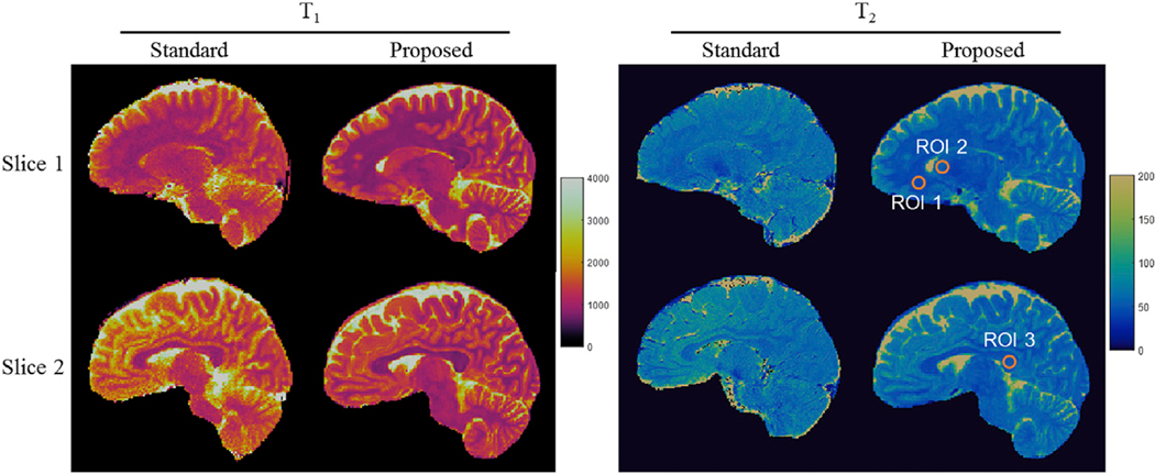
We further compared the T₁ and T₂ quantification obtained using the proposed method and the standard relaxometry methods. Two representative slices are shown in Fig. 11. Quantitative T₁ and T₂ values were also extracted through a region-of-interest (ROI) analysis and the results are presented in Table 2. Despite the difference in slice thickness between the methods (1 mm vs. 5 mm), the quantitative T₁ and T₂ results are generally in a good agreement in most of the brain regions.

Fig. 11.

Comparison of T₁ and T₂ maps obtained using the proposed 3D MRF and the standard relaxometry methods from the same subject. The results acquired at two different slices are presented. Three ROIs were drawn manually to extract quantitative T₁ and T₂ values from multiple brain tissues and the results are shown in Table 2.

Table 2.

Comparison of T₁ and T₂ relaxation times obtained between the proposed 3D MRF method and standard relaxometry methods.

	T1 (ms)		T2 (ms)
	Standard	MRF	Standard	MRF
ROI 1	883 ± 46	777 ± 27	51 ± 3	43 ± 1
ROI 2	1227 ± 82	1377 ± 75	62 ± 3	56 ± 3
ROI 3	844 ± 23	781 ± 41	54 ± 3	52 ± 2

4. Discussion

In this study, a rapid 3D MRF method with a spatial resolution of 1 mm³ was developed, which could provide whole-brain (18-cm volume) quantitative T₁ and T₂ maps in ~7 min. This is comparable or even shorter to the acquisition time of conventional T₁-weighted and T₂-weighted images with a similar spatial resolution. By leveraging both parallel imaging and deep learning techniques, the proposed method demonstrates improved performance as compared to the previously published methods (Ma et al., 2018). In addition, the processing time to extract T₁ and T₂ values was accelerated by more than 7 times with the deep learning approach as compared to the standard template matching method.

Two advanced techniques, parallel imaging and deep learning, were combined to accelerate high-resolution 3D MRF acquisitions with whole brain coverage. The 3D MRF sequence employed in this study was already highly accelerated for in-plane encoding with only one spiral arm acquired (R = 48). Therefore, more attention was paid to apply parallel imaging along the partition-encoding direction to further shorten the scan time. In addition, CNN has been shown capable of extracting features from complex MRF signals in both spatial and temporal domains that are needed for accurate quantification of tissue properties. This has been well demonstrated in the previous 2D MRF studies (Fang et al., 2019). With 3D acquisitions, spatial constraints from all three dimensions were utilized for tissue characterization. The integration of advanced parallel imaging and convolutional neural networks leads to 1) drastically reduced the amount of data needed for high-resolution MRF images and 2) extract more advanced features, achieving improved tissue characterization and accelerated T₁ and T₂ mapping using MRF. In addition to shortening MRF acquisitions in the temporal domain, the deep learning method also helps to eliminate some residual artifacts in T₂ maps after the GRAPPA reconstruction. This is consistent with recent findings that deep learning methods can be applied to reconstruct undersampled MR images and provide comparable results to conventional parallel imaging and compressed sensing techniques (Akçakaya et al., 2018; Eo et al., 2018; Hammernik et al., 2018; Quan et al., 2018; Schlemper et al., 2018).

Parallel imaging along partition direction was applied to accelerate 3D MRF acquisition with 1-mm isotropic resolution. Our results and others have shown that with such a high spatial resolution, the interleaved undersampling pattern with template matching does not resolve the aliasing artifacts in 3D imaging (Liao et al., 2017). By leveraging the sliding window reconstruction approach, previous studies have applied the Cartesian GRAPPA to reconstruct a 3D MRF dataset and a reduction factor of 3 was explored with the same spatial resolution (Liao et al., 2017). In the current study, advanced parallel imaging methods similar to the spiral GRAPPA was used. To compute GRAPPA weights, the calibration data was acquired from the central partitions and integrated into the image reconstruction to preserve tissue contrast. This approach does not rely on the sliding window method, which could potentially reduce the MRF sensitivity along the temporal domain (Liao et al., 2017). With the proposed approach, high-quality quantitative T₁ and T₂ maps were obtained with a reduction factor of 2 and some artifacts were found with a higher reduction factor of 3. The difference at the higher reduction factor, as compared to findings in the previous study (Liao et al., 2017), is likely due to different strategies to accelerate data acquisition. Specifically, only 192 time points were acquired to form MRF signal evolution in this study, while ~420 points were used in the previous study (Liao et al., 2017). More time points can be utilized to mitigate aliasing artifacts in the final quantitative maps, but at a cost of a longer sampling time for each partition and thus total acquisition time.

A modified 3DMRF-DL sequence was developed to acquire the necessary dataset to train the CNN model that can be applied to prospectively accelerated 3D MRF data. With the 3DMRF-S sequence, a short waiting time (typically 2–3 s) was applied between the acquisitions of different partitions for longitudinal relaxation. Due to the incomplete T₁ relaxation with this short waiting time, the retrospectively shortened dataset acquired with this sequence does not match with the prospectively acquired accelerated data even with the same number of time points. One potential method to mitigate this problem is to acquire two separate scans, one accelerated scan with reduced time points and the other with all N points to extract ground truth maps. However, considering the long scan time to obtain the ground truth maps, this approach will be sensitive to subject motion between scans. Even for a small motion, the corresponding tissue property maps could potentially lead to an incorrect estimation of parameters in the CNN model. Image registration can be applied to correct motions between scans, but variations could be introduced during the registration process. The proposed 3DMRF-DL method provides an alternative solution for this issue and generates the necessary data without the concern of relative motion in the CNN training dataset. While extra scan time is needed with an additional pulse sequence section, the total acquisition is the identical to acquire two separate scans to solve this issue.

In the proposed 3DMRF-DL sequence, a preparation module containing the pulse sequence section for the first M time points was added before the actual data acquisition section. One potential concern with this approach is whether one preparation module will be sufficient to generate the same spin history as the prospectively accelerated scans. Previous studies have shown that when computing the dictionary for 3D MRF, a simulation with one such preparation module is sufficient to reach the magnetization state for calculation of the MRF signal evolution in actual acquisitions (Liao et al., 2017). Our simulation (Fig. S1) confirms that the signal evolution obtained from the proposed 3DMRF-DL method matched well with the prospectively accelerated 3DMRF-S method. All of these findings suggest that the one preparation module added in the 3DMRF-DL sequence is sufficient to generate the magnetization state as needed.

To implement the 3DMRF-DL method to acquire the training dataset, the number of time points (M), which is also the number of time points used in the prospectively accelerated scan, needs to be determined first. This can be achieved by acquiring multiple training datasets with different M values and comparing the quantitative results in between. However, the data acquisition process for this approach is time-consuming and the comparison is also sensitive to the quality of different training datasets. Alternatively, this optimal M value can be identified using the 3DMRF-S method as performed in this study. While small variation exists in MRF signal acquired with this approach as compared to the 3DMRF-DL method, the difference is relatively small in terms of MRF signal evolution and magnitude (supplemental materials). Therefore, it is reasonable to use the 3DMRF-S method to estimate the optimal M value. Only one training dataset is needed and retrospective data shortening can be performed to compare the results from different time points.

Subject motion in clinical imaging presents one of the major challenges for high-resolution MR imaging. Compared to the standard MR imaging with Cartesian sampling, MRF utilizes a non-Cartesian spiral trajectory for in-plane encoding, which is known to yield better performance in the presence of motion (Ma et al., 2013). The template matching algorithm used to extract quantitative tissue properties also provides a unique opportunity to reduce motion artifacts. As demonstrated in the original 2D MRF paper (Ma et al., 2013), the motion-corrupted time frames behaved like noise during the template matching process and accurate quantification was obtained in spite of subject motion. However, the performance of 3D MRF in the presence of motion has not been fully explored. A recent study showed that 3D MRF with linear encoding along partition-encoding direction is also sensitive to motion artifacts (Cao et al., 2019), and the degradation in T₁ and T₂ maps is likely dependent on the magnitude and timing of the motion during the 3D scans (Mehta et al., 2018). The 3D MRF approach introduced in this study will help to reduce motion artifacts with the accelerated scans. The lengthy acquisition of the training dataset acquired in this study is more sensitive to subject motion. While no evident artifacts were noticed with all subjects scanned in this study, further improvement in motion robustness is needed for 3D MRF acquisitions.

Another factor that could influence the accuracy of MRF quantification is the selection of T₁ and T₂ step sizes in the dictionary. Since not every possible combination of T₁ and T₂ values are included in the dictionary, this may affect the values in the ground truth maps and therefore the values derived with the CNN method. Future studies will be performed to evaluate the effect of step sizes on the accuracy of tissue quantification using the proposed method.

There are some limitations in our study. First, the network structure and training parameters for the deep learning approach were largely adopted from the previous 2D MRF study (Fang et al., 2019). While a similar MRF acquisition method was used, differences in spatial resolution, SNR, and the number of time points could potentially introduce differences in the optimized CNN setting. Moreover, in considering the memory size in the GPU card, MRF data from three contiguous slices were used as the input in this study. Input dataset with different number of slices or a true 3D CNN network could influence the network performance and future studies will be performed to optimize the CNN model specifically for 3D MRF acquisitions. In addition, some acquisition parameters, such as the 2-sec waiting time between partitions, were also adopted from previous studies (Liao et al., 2017; Ma et al., 2018) and these can be further optimized in future studies. Second, all experiments and development were performed on normal subjects and its application for patients with various pathologies needs to be evaluated. Finally, the current study focused on quantification of tissue T₁ and T₂ values while MRF has been applied for quantification of many other tissue contrasts including T₂*, diffusion, perfusion, and magnetic transfer (Heo et al., 2019; Wang et al., 2018; Wright et al., 2018). Longer acquisition times are required to extract more tissue properties with MRF and the application of the proposed method to accelerate these acquisitions will be explored in the future.

In conclusion, a high-resolution 3D MR Fingerprinting technique, combining parallel imaging and deep learning, was developed for rapid and simultaneous quantification of T₁ and T₂ relaxation times. Our results show that with the integration of parallel imaging and deep learning techniques, whole-brain quantitative T₁ and T₂ mapping with 1-mm isotropic resolution can be achieved in ~7 min, which is feasible for routine clinical practice.

References

- Akçakaya M, Moeller S, Weingäartner S, Uğurbil K, 2018. Scan-specific robust artificial-neural-networks for k-space interpolation (RAKI) reconstruction: database-free deep learning for fast imaging. Magn. Reson. Med 1–15. [DOI] [PMC free article] [PubMed] [Google Scholar]
- Badve C, Yu A, Dastmalchian S, Rogers M, Ma D, Jiang Y, Margevicius S, Pahwa S, Lu Z, Schluchter M, Sunshine XJ, Griswold M, Sloan A, Gulani V, 2017. MR fingerprinting of adult brain tumors: initial experience. Am. J. Neuroradiol 38, 492–499. [DOI] [PMC free article] [PubMed] [Google Scholar]
- Cao X, Ye H, Liao C, Li Q, He H, Zhong J, 2019. Fast 3D brain MR fingerprinting based on multi-axis spiral projection trajectory. Magn. Reson. Med 1–13. [DOI] [PubMed] [Google Scholar]
- Chen Y, Chen M-H, Baluyot K, Potts T, Jimenez J, Lin W, 2019a. MR Fingerprinting enables quantitative measures of brain tissue relaxation times and myelin water fraction in early brain development. Neuroimage 186, 782–793. [DOI] [PubMed] [Google Scholar]
- Chen Y, Jiang Y, Pahwa S, Ma D, Lu L, Twieg MD, Wright KL, Seiberlich N, Griswold MA, Gulani V, 2016. MR fingerprinting for rapid quantitative abdominal imaging. Radiology 279, 278–286. [DOI] [PMC free article] [PubMed] [Google Scholar]
- Chen Y, Lee GR, Wright KL, Badve C, Nakamoto D, Yu A, Schluchter MD, Griswold MA, Seiberlich N, Gulani V, 2015. Free-breathing liver perfusion imaging using 3-dimensional through-time spiral generalized autocalibrating partially parallel acquisition acceleration. Investig. Radiol 50, 367–375. [DOI] [PMC free article] [PubMed] [Google Scholar]
- Chen Y, Panda A, Pahwa S, Hamilton JI, Dastmalchian S, Mcgivney D, Ma D, Batesole J, Seiberlich N, Griswold MA, Plecha D, Gulani V, 2019b. 3D magnetic resonance fingerprinting for quantitative breast imaging. Radiology 290, 33–40. [DOI] [PMC free article] [PubMed] [Google Scholar]
- Cohen O, Zhu B, Rosen MS, 2018. MR fingerprinting deep RecOnstruction NEtwork (DRONE). Magn. Reson. Med 80, 885–894. [DOI] [PMC free article] [PubMed] [Google Scholar]
- Deichmann R, Good CD, Josephs O, Ashburner J, Turner R, 2000. Optimization of 3-D MP-RAGE sequences for structural brain imaging. Neuroimage 12, 112–127. [DOI] [PubMed] [Google Scholar]
- Eo T, Jun Y, Kim T, Jang J, Lee HJ, Hwang D, 2018. KIKI-net: cross-domain convolutional neural networks for reconstructing undersampled magnetic resonance images. Magn. Reson. Med 80, 2188–2201. [DOI] [PubMed] [Google Scholar]
- Fang Z, Chen Y, Liu M, Xiang L, Zhang Q, Wang Q, Lin W, Shen D, 2019. Deep learning for fast and spatially-constrained tissue quantification from highly-accelerated data in magnetic resonance fingerprinting. IEEE Trans. Med. Imaging (in press). [DOI] [PMC free article] [PubMed] [Google Scholar]
- Fischl B, Salat DH, Busa E, Albert M, Dieterich M, Haselgrove C, van der Kouwe A, Killiany R, Kennedy D, Klaveness S, Montillo A, Makris N, Rosen B, Dale AM, 2002. Whole brain segmentation: automated labeling of neuroanatomical structures in the human brain. Neuron 33, 341–355. [DOI] [PubMed] [Google Scholar]
- Hamilton JI, Jiang Y, Chen Y, Ma D, Lo WC, Griswold M, Seiberlich N, 2017. MR fingerprinting for rapid quantification of myocardial T1, T2, and proton spin density. Magn. Reson. Med 77, 1446–1458. [DOI] [PMC free article] [PubMed] [Google Scholar]
- Hammernik K, Klatzer T, Kobler E, Recht MP, Sodickson DK, Pock T, Knoll F, 2018. Learning a variational network for reconstruction of accelerated MRI data. Magn. Reson. Med 79, 3055–3071. 10.1002/mrm.26977. [DOI] [PMC free article] [PubMed] [Google Scholar]
- Heo HY, Han Z, Jiang S, Schäar M, van Zijl PCM, Zhou J, 2019. Quantifying amide proton exchange rate and concentration in chemical exchange saturation transfer imaging of the human brain. Neuroimage 189, 202–213. [DOI] [PMC free article] [PubMed] [Google Scholar]
- Hoppe E, Korzdorfer G, Nittka M, Wirfl T, Wetzl J, Lugauer F, Schneider M, Pfeuffer J, Maier A, 2018. Deep learning for Magnetic Resonance Fingerprinting: accelerating the reconstruction of quantitative relaxation maps. Int. Soc. Magn. Reson. Med p2791. [Google Scholar]
- Hoppe E, Körzdörfer G, Würfl T, Wetzl J, Lugauer F, Pfeuffer J, Maier A, 2017. Deep learning for magnetic resonance fingerprinting: a new approach for predicting quantitative parameter values from time series. Stud. Health Technol. Inform 243, 202–206. [PubMed] [Google Scholar]
- Jiang Y, Ma D, Seiberlich N, Gulani V, Griswold MA, 2015. MR fingerprinting using fast imaging with steady state precession (FISP) with spiral readout. Magn. Reson. Med 74, 1621–1631. [DOI] [PMC free article] [PubMed] [Google Scholar]
- Körzdörfer G, Kirsch R, Liu MK, Pfeuffer J, Hensel B, 2019. Reproducibility and repeatability of MR fingerprinting relaxometry in the human brain. Radiology 292, 429–437. [DOI] [PubMed] [Google Scholar]
- Liao C, Bilgic B, Manhard MK, Zhao B, Cao X, Zhong J, Wald LL, Setsompop K, 2017. 3D MR fingerprinting with accelerated stack-of-spirals and hybrid sliding-window and GRAPPA reconstruction. Neuroimage 162, 13–22. [DOI] [PMC free article] [PubMed] [Google Scholar]
- Liao C, Wang K, Cao X, Li Y, Wu D, Ye H, Ding Q, He H, Zhong J, 2018. Detection of lesions in mesial temporal lobe epilepsy by using MR fingerprinting. Radiology 288, 804–812. [DOI] [PubMed] [Google Scholar]
- Ma D, Gulani V, Seiberlich N, Liu K, Sunshine JL, Duerk JL, Griswold MA, 2013. Magnetic resonance fingerprinting. Nature 495, 187–192. [DOI] [PMC free article] [PubMed] [Google Scholar]
- Ma D, Jiang Y, Chen Y, McGivney D, Mehta B, Gulani V, Griswold M, 2018. Fast 3D magnetic resonance fingerprinting for a whole-brain coverage. Magn. Reson. Med 79, 2190–2197. [DOI] [PMC free article] [PubMed] [Google Scholar]
- Ma D, Jones SE, Deshmane A, Sakaie K, Pierre EY, Larvie M, McGivney D, Blümcke I, Krishnan B, Lowe M, Gulani V, Najm I, Griswold MA, Wang ZI, 2019. Development of high-resolution 3D MR fingerprinting for detection and characterization of epileptic lesions. J. Magn. Reson. Imaging 49, 1333–1346. [DOI] [PubMed] [Google Scholar]
- McGivney D, Pierre E, Ma D, Jiang Y, Saybasili H, Gulani V, Griswold M, 2014. SVD compression for magnetic resonance fingerprinting in the time domain. IEEE Trans. Med. Imaging 0062, 1–13. [DOI] [PMC free article] [PubMed] [Google Scholar]
- Mehta BB, Ma D, Pierre EY, Jiang Y, Coppo S, Griswold MA, 2018. Image reconstruction algorithm for motion insensitive MR Fingerprinting (MRF): MORF. Magn. Reson. Med 80, 2485–2500. [DOI] [PubMed] [Google Scholar]
- Pierre E, Ma D, Chen Y, Badve C, Griwold MA, 2016. Multiscale reconstruction for magnetic resonance fingerprinting. Magn. Reson. Med 75, 2481–2492. [DOI] [PMC free article] [PubMed] [Google Scholar]
- Quan TM, Nguyen-Duc T, Jeong WK, 2018. Compressed sensing MRI reconstruction using a generative adversarial network with a cyclic loss. IEEE Trans. Med. Imaging 37, 1488–1497. [DOI] [PubMed] [Google Scholar]
- Schlemper J, Caballero J, Hajnal JV, Price A, Rueckert D, 2018. A deep cascade of convolutional neural networks for dynamic MR image reconstruction. IEEE Trans. Med. Imaging 37, 491–503. [DOI] [PubMed] [Google Scholar]
- Seiberlich N, Lee G, Ehses P, Duerk JL, Gilkeson R, Griswold M, 2011. Improved temporal resolution in cardiac imaging using through-time spiral GRAPPA. Magn. Reson. Med 66, 1682–1688. [DOI] [PMC free article] [PubMed] [Google Scholar]
- Wang CY, Coppo S, Mehta BB, Seiberlich N, Yu X, Griswold MA, 2018. Magnetic resonance fingerprinting with quadratic RF phase for measurement of T 2 * simultaneously with δ f, T 1, and T 2. Magn. Reson. Med 81, 1849–1862. [DOI] [PMC free article] [PubMed] [Google Scholar]
- Wright KL, Jiang Y, Ma D, Noll DC, Griswold MA, Gulani V, Hernandez-Garcia L, 2018. Estimation of perfusion properties with MR fingerprinting arterial spin labeling. Magn. Reson. Imaging 50, 68–77. [DOI] [PMC free article] [PubMed] [Google Scholar]
- Yu AC, Ponsky LE, Dastmalchian S, Rogers M, Mcgivney D, Griswold MA, 2017. Development of a combined MR fingerprinting and diffusion examination for prostate. Radiology 283, 729–738. [DOI] [PMC free article] [PubMed] [Google Scholar]
Associated Data
This section collects any data citations, data availability statements, or supplementary materials included in this article.