MRI-Based Deep Learning Segmentation and Radiomics of Sarcoma in Mice

Short abstract

Small-animal imaging is an essential tool that provides noninvasive, longitudinal insight into novel cancer therapies. However, considerable variability in image analysis techniques can lead to inconsistent results. We have developed quantitative imaging for application in the preclinical arm of a coclinical trial by using a genetically engineered mouse model of soft tissue sarcoma. Magnetic resonance imaging (MRI) images were acquired 1 day before and 1 week after radiation therapy. After the second MRI, the primary tumor was surgically removed by amputating the tumor-bearing hind limb, and mice were followed for up to 6 months. An automatic analysis pipeline was used for multicontrast MRI data using a convolutional neural network for tumor segmentation followed by radiomics analysis. We then calculated radiomics features for the tumor, the peritumoral area, and the 2 combined. The first radiomics analysis focused on features most indicative of radiation therapy effects; the second radiomics analysis looked for features that might predict primary tumor recurrence. The segmentation results indicated that Dice scores were similar when using multicontrast versus single T2-weighted data (0.863 vs 0.861). One week post RT, larger tumor volumes were measured, and radiomics analysis showed greater heterogeneity. In the tumor and peritumoral area, radiomics features were predictive of primary tumor recurrence (AUC: 0.79). We have created an image processing pipeline for high-throughput, reduced-bias segmentation of multiparametric tumor MRI data and radiomics analysis, to better our understanding of preclinical imaging and the insights it provides when studying new cancer therapies.

Introduction

Because imaging is a standard means for assessing disease state and therapeutic response in clinical oncology, small-animal imaging for coclinical cancer trials enhances the simulation of clinical practice in animals. High-resolution images can noninvasively describe tumor morphology and composition, as well as how tumors change over time or with treatment.

Magnetic resonance imaging (MRI) is the clinically preferred method for imaging soft tissue sarcomas owing to its excellent soft tissue contrast (1). Assessing treatment response requires tumor measurements that are both accurate and precise. Manual segmentations suffer from variability that is in part due to individual human rater biases. In the clinic, tumor regions are often identified with input provided by radiologists or radiation oncologists. However, advances in computer vision have made automated segmentation processes possible. Specifically, segmentation algorithms based on convolutional neural networks (CNNs) have shown comparable efficacy in identifying tumors as other automated methods (2). Several CNN-based methods have been proposed for tumor segmentation from multicontrast MRI, based on both 2D slices (3) or 3D volumes (4). Many current architectures for tumor segmentation use a patch-based approach, in which a 2D or 3D patch is processed by convolutional and fully connected layers to classify the center pixel of the patch (3, 5). Other networks operate semantic-wise by classifying each pixel in an input image or a patch using fully convolutional networks or U-nets (2, 6). Deep learning solutions are particularly attractive for processing multichannel, volumetric image data, where conventional processing methods are often computationally expensive (7).

The extraction of high-dimensional biomarkers using radiomics can identify tumor signatures that may be able to monitor disease progression or response to therapy or predict treatment outcomes (8, 9). Radiomics analysis generates complex high-dimensional data, and trends are often difficult to extract. The utility of radiomics benefits greatly from the use of machine learning algorithms (10). In this way, radiomics provides an exciting approach for identifying and developing imaging biomarkers in the context of precision medicine.

Our group has established quantitative imaging techniques for the preclinical arm of a coclinical sarcoma trial studying the treatment synergy between immune checkpoint blockade with an antibody against programmed cell death protein 1 (PD-1) and radiation therapy (RT) in a genetically engineered mouse model of soft tissue sarcoma (11). Our first objective was to develop and evaluate a deep learning method based on CNNs to perform automatic tumor segmentation of preclinical MRI data acquired in these sarcomas. The high-throughput capacity of a fully automated segmentation pipeline offers a significant time advantage in a large-scale study, as is often the case when studying cancer therapeutics. Even more importantly, a CNN-based segmentation protocol has the advantage of removing observer bias, which can have a significant effect on defining tumor tissue in magnetic resonance (MR) images (12).

The second objective was to perform radiomics analyses on the acquired MRI data sets. Recently, radiomics analysis has been successfully applied to clinical sarcoma data (13). There is evidence that radiomics features extracted from MRI may serve as biomarkers for predicting overall survival in patients with soft tissue sarcomas (14). To the best of our knowledge, no radiomics studies exist on mouse models of sarcomas. This study describes and evaluates our small-animal MRI-based image analysis pipeline on sarcomas treated with RT, including automated tumor segmentation and radiomics analysis.

Methods

Sarcoma Model and Experimental Protocol

The preclinical arm of our coclinical trial uses a genetically engineered model of soft tissue sarcoma developed in p53^fl/fl mice. Primary sarcoma lesions were generated in the hind limb by intramuscular delivery of Adeno-Cre followed by injection of the carcinogen 3-methylcholanthrene (p53/MCA model) (15). Tumors resembling human undifferentiated pleomorphic sarcoma developed ∼8–12 weeks after injection. Imaging studies were initiated when tumors were palpable (>100 mg), continuing through subsequent stages of disease progression. Mice were killed at the end of the study either once the tumor burden became excessive or 6 months after surgery. Excessive burden was defined as recurrent tumors >1.5 cm in length or presence of large lung metastasis.

Three MRI images, 1 T2-weighted, and 2 T1-weighted (before and after contrast injection), were obtained 1 day before delivering RT (20 Gy) on a small-animal irradiator (Precision X-ray X-RAD 320) with 100 kV. One week later, the mice were reimaged with MRI using the same imaging protocol. After the second MRI, the primary tumor was surgically removed by amputating the tumor-bearing hind limb, and mice were followed for up to 6 months. Some mice developed local recurrence of the primary tumors near the site of amputation or developed distant metastases.

Multicontrast MRI

All MR studies were performed on a 7.0 T Bruker Biospec small-animal MRI scanner (Bruker Inc., Billerica, MA), with a 20-cm bore, equipped with an AVANCE III console, using Paravision 6.0.1, and a 12-cm-inner-diameter gradient set capable of delivering 440 mT/m. Tumor images were acquired using the 4-element surface coil array (receive), coupled with the 72-mm linear volume (transmit) coil. All animal handling and imaging procedures were performed according to protocols approved by the Duke Institutional Animal Care and Use Committee (IACUC). Acquisition parameters have previously been described in detail (11) and are as follows:

1. T1-weighted: A 2D T1 FLASH sequence was performed with echo time of 4.5 milliseconds and repetition time of ∼0.9 seconds. A fixed field of view of 28 × 28 mm (read and phase) was selected to ensure full coverage of the tumor volume with reasonable margins. In-plane resolution was 100 µm over 60, 300-µm thick axial slices (slice direction typically along the tibia). Three images were acquired and averaged to reduce the effects of motion (which are limited in the hind limb). The flip angle was 30°.

2. T2-weighted: A 2D T2 TurboRARE sequence was performed with an effective echo time of 45 milliseconds and repetition time of ∼8.6 seconds. The echo spacing for the T2TurboRARE sequence was 15 milliseconds. Scans were performed with identical slice geometry and field of view to the preceding T1 sequence. As with the T1 images, 3 averages were acquired, with a RARE factor of 8.

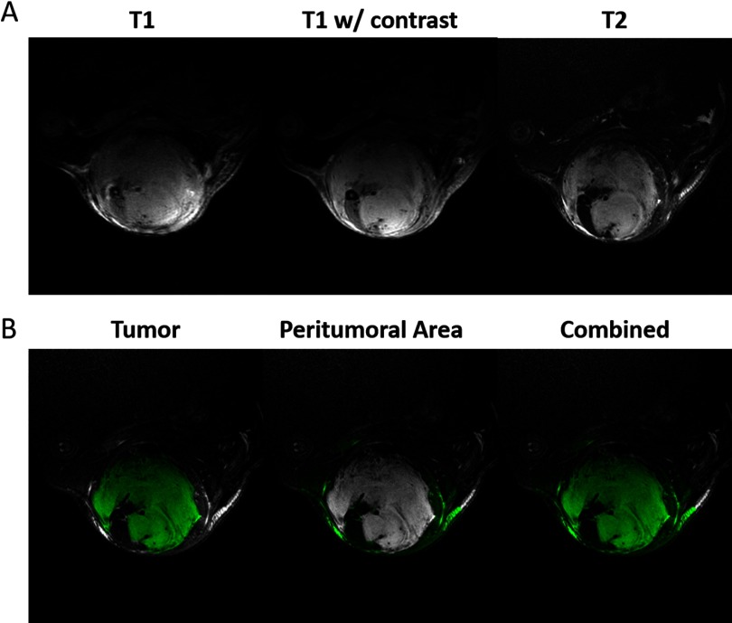
Following the acquisition of nonenhanced scans, T1 contrast enhancement was achieved via injection of Gd-DTPA at 0.5 mmol/kg via the tail vein catheter, which was placed under anesthesia before imaging. Contrast was injected at 2.5 mL/min and allowed to circulate for 3 minutes before a second T1-weighted scan to allow peak enhancement. The MR images were bias-corrected in a 3D Slicer using the N4 algorithm (16). The sarcoma tumors were next segmented using the T2-weighted images in 2 steps: first, semiautomatic segmentation was performed via the 3D Slicer with the GrowCut tool (17), and second, an observer refined the segmentations by hand. Two researchers acted as observers to create binary segmentation labels with initial guidance from a radiation oncologist experienced with mouse models. In total, 70 manual segmentations were created to serve as the ground truth to train the CNN, including both pre- and post-RT images. Examples of each multicontrast MR image together with the tumor segmentation used as labels for training are shown in Figure 1A. An overview of the data used for this study is given in Table 1. Although we have used 79 mice with tumors, only 62 mice had 2 MRI scans and 42 mice qualified for radiomics analysis.

Figure 1.

Multi-contrast magnetic resonance imaging (MRI) images of soft tissue sarcomas. Sarcomas imaged with 3 magnetic resonance (MR) protocols show differences in image contrast (A). Examples of the regions used to calculate radiomics features for each tumor (B). Features were calculated for the tumor, peritumoral area, and the union of those regions. The tumor segmentation was performed using semiautomatic methods and cleaned by hand. Air was excluded from the dilated masks via thresholding.

Table 1.

Overview of Study Mice and Scan Segmentations Used for Training and Radiomics

Mice			Scans for Segmentation
TotalMice	Mice with 2 scans	Mice forradiomicsa	MRSets	Manual Segmentations	Unique ManuallySegmented Scansb	Overlap withradiomics scans	K-FoldsValidation Size	K-FoldsTest Size
79	62	42	141	70	49	39	6	12

^aThese mice were not excluded for surgical complications or other health reasons.

^b21 of these scans were segmented twice, once by each reader for a total of 70 segmentations.

CNN-Based Segmentation

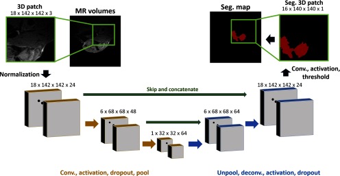
We have implemented a 3D fully convolutional U-net network similar to Ronneberger et al. (18) using Tensorflow (19) to segment soft tissue sarcomas in mice¹. To assess the utility of collecting multiple scans with different contrasts, we have compared the segmentation performance of networks trained on 2 sets of images. The network is presented with inputs of either only T2-weighted images or the MRI images with 3 different contrasts (see Figure 1A). In the case of multicontrast segmentation, the 3 images are concatenated together as channels of a single image, i.e., the network takes a single, 4-dimensional (read, phase, slice, channel) input. Image intensities are normalized on each image volume to map voxel values to within a standard, zero-centered reference scale. This mapping serves to address differences in bias between images of similar contrast and optimize image values for consistent CNN processing. Our network operates on 3D image patches (dimensions, in voxels: 142, 142, 18) selected out of larger image volumes (280, 280, 60). The output of the network is a single 3D segmentation map, showing the probability that a given pixel belongs to the background or foreground (tumor). Thresholding this map yields a binary segmentation from which the tumor volume and radiomics features are determined.

The network comprises 2 halves: an encoder with convolutional layers and max pooling and a decoder layer with deconvolutional layers and up-sampling operations. The structure of the network is shown in Figure 2. The use of multiple max pooling operations (size: 2 × 2 × 2) allows for detection of multiscale features using small, 3 × 3 × 3, convolution kernels, greatly increasing the computational efficiency of the network. The number of convolution filters and, by extension, feature maps, are increased after pooling to preserve information found at finer resolutions. Activation layers after each convolution operation were set as rectilinear activation units. The final activation is a sigmoid function, setting the network’s output to be within the range of 0 to 1.

Figure 2.

Convolutional Neural Network (CNN) architecture used for segmentation. Volumetric patches are taken from either single or multicontrast MR images. The patches are normalized and passed through a successive 3D convolutional encoder (gold) and deconvolutional decoder (blue). Skip connections (green) take feature maps from the encoder and concatenate them with decoder feature maps before deconvolution operations. All convolution/deconvolution operations are performed with 3 × 3 × 3 kernels with a stride of 1 × 1 × 1.

To increase the amount of information available to the decoder portion of the network, skip connections are present. Skip connections take a set of feature maps from the encoder and concatenate them with features maps in the decoder. These connections reintroduce higher frequency data directly into the decoder and have been shown to increase accuracy for segmentation tasks (18). We have tested the performance of this network both with and without skip connections.

Care was taken to prevent the network from overfitting. To this end, spatial dropout was applied before max pooling and upsampling layers. Spatial dropout is a variation of classical neural network dropout that is more applicable to CNNs. Spatial dropout will randomly zero out feature maps, forcing the network to learn redundancy in identifying important image features rather than overfitting to the peculiarities native to the training data (20, 21).

The selection of an appropriate loss function is critical for designing an effective CNN model. We chose to train and compare models using 2 loss metrics: Dice loss (22), which is a measure of similarity between the prediction and label, and cross entropy (23) which is based on the distributions of the prediction and label images. Both are popular cost functions for segmentation tasks (3, 4, 6, 18). The Dice score for predictions P ∈ {0, 1} and the expert’s consensus ground truth T ∈ {0, 1} are defined as:

$$D=\frac{2|P\cap T|}{\left|P\right|+\left|T\right|}$$

where $\left|P\right|$ and $\left|T\right|$ represent the cardinality of the prediction and ground truth sets, respectively. Predictions that perfectly match the ground truth will have a Dice coefficient of 1, whereas predictions with little intersection with the ground truth will have a score near 0. Dice loss requires the use of binary inputs, so network outputs were thresholded by 0.5 before loss is computed. For use as a loss function, we used the Dice score minus one. Cross entropy loss is computed as the measure of similarity between estimated probabilities and ground truth.

We have trained and tested our network using a single MR image contrast (T2-weighted) and all 3 contrasts (T1-weighted, T1-weighted with contrast, and T2-weighted). Visually, the T2-weighted images show the highest contrast for tumor detection (Figure 1A); however, we aimed to determine the utility of including the T1-weighted images for tumor segmentation, as they are typically included in clinical MRI acquisition protocols.

In total, 8 networks were trained and evaluated. These networks iterated combinations of 3 parameters: Dice versus cross entropy loss functions, networks with skip connections versus those without, and multicontrast versus T2-only MR images as inputs. Training data comprised a random selection of 70% training data, 20% validation data, and 10% test data. All networks were trained for 600 epochs, requiring between 6 to 9 hours each. Networks were trained with a batch size of 20 and a learning rate of 1e-4. Early stopping was used by saving network weights at validation loss minimums. Training was performed on a stand-alone workstation equipped with an NVidia Titan RTX GPU (NVidia, Santa Clara, CA).

The output of each segmentation CNN is a set of probabilities, one for each input voxel. Once the CNN was trained, a decision threshold was found to convert floating point probability maps to binary segmentations. The decision threshold is selected to maximize the fit of the predicted segmentation, and in this case, to maximize the Dice coefficient between the predicted results and the label. The threshold is calculated by running the training data through the trained network and generating precision/recall curves. The threshold at the intersection of precision and recall gives the highest agreement between the predicted segmentation and label images. This threshold gives the highest true-positive and lowest false-positive performance, maximizing the quality of the segmentation.

The images in our data set contain a single primary soft tissue sarcoma located in the hind leg, and the segmentation ground truth of these tumors is continuous. Because the CNN processes the image volume in patches without spatial references, the resulting segmentations are not guaranteed to have these properties, and the small structures outside the tumor are occasionally misclassified. To address this, after recomposing the image volume from processed patches, a postprocessing step was implemented, which rejected all but the largest continuous region in the predicted segmentation.

To provide uniform treatment of mice for subsequent radiomics analysis, the top-performing segmentation network was selected and trained again, this time using 5-fold cross validation with 10% validation and 20% testing splits (Table 1). This was necessary owing to the overlap in training data and valid radiomics sets. Each trained network would be responsible for processing only its test set, allowing these networks to cover the entirety of the radiomics data. Data that did not contribute to radiomics analysis were used for only training. Scans that contributed to radiomics analysis but did not have an associated hand segmentation were processed via an ensemble of the 5 networks via majority voting.

Segmentation Quality Metrics.

We have evaluated the performance of our CNN segmentations using several metrics, the simplest of which is binary accuracy. Binary accuracy is given as the percent of voxels correctly classified by the network. The predicted probabilities are thresholded by 0.5 before calculating this metric.

We also included the Dice score, which is a standard evaluation metric in the medical imaging and computer vision communities. In addition to being used as an image quality metric, Dice was used as a loss function for half of our networks. We have also calculated the volume overlap error (VOE), also called the Jaccard similarity score, given by the intersection over the union of the ground truth (T) and prediction (P):

$$VOE=\frac{|P\cap T|}{\left|P\cup T\right|}$$

Radiomics

Using the CNN-produced segmentation maps, we performed radiomics analysis for multiple regions (Figure 1B): (A) tumor; (B) peritumoral area obtained by morphological dilation that spans 3 mm outside of the tumor; and (C) tumor combined with the peritumoral area. Each of these regions serve as masks in which to compute radiomics features. Dilation was performed using the scikit-image Python package (24). Before computing radiomics features, the MR images were normalized to account for variations in intensities, which can substantially impact feature extraction and classification. Normalization was performed by zero-centering image data and scaling values to have unit standard deviation σ. Intensity outliers (values outside ±3σ) were excluded from calculations as described in a study (25). Radiomics features were calculated using the PyRadiomics package (26). From each MR contrast image, 107 radiomics features were calculated, creating a high-dimensional feature space. The multicontrast data were appended to create a single feature vector for each data set (321 features). All analysis was performed using multicontrast data. The extracted features were computed from normalized images only and did not include those calculated from derivative or filtered images (e.g., Laplacian of Gaussian, wavelet, etc.).

Our first analysis focused on determining which radiomics features are the most affected by RT. Radiomics features calculated from pre- and post-RT sets were compared to find the features that changed in a statistically significant manner, as determined by paired t tests with multiple t test corrections.

Our second analysis aimed to determine if differences in radiomics features showed promise for predicting which individuals on study would develop a recurrence of the primary tumor following surgical resection. Features selection using minimum redundancy–maximum relevance (mRMR) (27) was performed on the radiomics features to rank features in an effort to reduce redundancy and increase relevance based on recurrence. To visualize differences between groups of mice with and without local recurrence, correlation maps were computed using the 200 most relevant radiomics features selected via mRMR. For prediction of primary tumor recurrence, the top 10 features were used. The optimal number of features for prediction was found via a search that used from 2 to 200 features to maximize the area under the curve (AUC) of the receiver operating characteristic (ROC) curve. Two types of classifiers, based on simple neural networks (NNs) and support vector machines (SVMs), were used to create models predicting primary tumor recurrence. The models were trained using stratified K-fold validation. Because the quantity of data was not large by machine learning standards (data from 42 mice), each model was trained 5 times de novo. The data were split into training (75%) and validation (25%) sets, which were cycled for each training and selected to contain similar numbers of recurrences and nonrecurrences. The performance of the prediction models based on NNs or SVMs was assessed using the AUC of the ROC curves. Training and validation were performedusing radiomics vectors from each of the 3 regions, that is, tumor, peritumoral area, and both combined, as illustrated by Figure 1B.

Results

CNN Segmentation

The measure of agreement between the label and predicted segmentation for each network trained is given with metrics of precision, recall, Dice, and VOE. These values were calculated on the test set using all 8 networks trained (Table 2). Ideal metrics would have precision and recall be close to 1 and about equal. The closeness of these 2 values represents the quality of the decision threshold that was used for these data sets. Dice and VOE scores are shown to be significantly higher for the network with skip connections. In addition, the networks trained using multicontrast data performed better than those trained using only T2-weighted images. Differences in loss function between networks was shown to be small, with cross entropy being slightly favored. The results in the table were calculated after postprocessing image volumes to remove all but the largest continuous segmentation region. This step improved segmentation performance, increasing average AUC for ROC by 0.7%, Dice by 2.2%, and VOE by 0.8%.

Table 2.

Comparison of the Networks Trained for Sarcoma Segmentation

Cost	Data	Network	Threshold	Precision	Recall	AUC	Dice	VOE
Dice	Multi-contrast	No skip	0.900	0.833	0.820	0.957	0.827	0.994
		Skip	0.995	0.891	0.826	0.979	0.857	0.995
	T2 only	No skip	0.900	0.849	0.787	0.950	0.817	0.994
		Skip	0.998	0.906	0.776	0.977	0.836	0.994
Cross Entropy	Multi-contrast	No skip	0.656	0.814	0.858	0.996	0.835	0.994
		Skip	0.540	0.869	0.856	0.998	0.863	0.995
	T2 only	No skip	0.636	0.833	0.803	0.992	0.818	0.993
		Skip	0.516	0.873	0.849	0.997	0.861	0.995

Values have been calculated from the test set which contains 10% (ie, 7) image sets. In this data set, the network trained with cross entropy loss, skip connections, and on multicontrast images performed best according to 4 of the 5 metrics used in the current study.

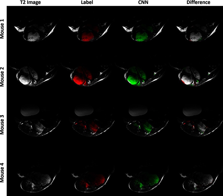
The best performing network, multicontrast with skip connections trained with cross-entropy loss, was retrained using 5-fold cross validation. The results are given in Table 3. CNN segmentations from 4 test volumes as computed with the k-fold networks are shown in Figure 3. The ground truth and predicted segmentations largely agree, with the greatest disagreement occurring on tumor edges and small extrusions. Visually, the CNN output and the original segmentation labels are generally well-matching, with only minor discrepancies. The average time required to process a single scan was 0.53 seconds.

Figure 3.

Results of CNN segmentation comparing the ground truth (label, red) with the model predictions (green) for the k-fold networks trained on cross entropy loss with skip connections and multicontrast data. Each row shows a single slice taken from separate tumor in the test set. The T2-weighted image is given for reference. The difference column shows errors in the CNN segmentation relative to the label: red for false negatives and green for false positives.

Table 3.

Performance of 5-Fold Cross Validation for the Network with Skip Connections Trained on Multi-Contrast Images with Cross Entropy Loss

Threshold	Precision	Recall	AUC	Dice	VOE
0.4220 ± 0.0680	0.8365 ± 0.0414	0.8497 ± 0.0260	0.9972 ± 0.0014	0.8422 ± 0.0187	0.9933 ± 0.0009

Radiomics

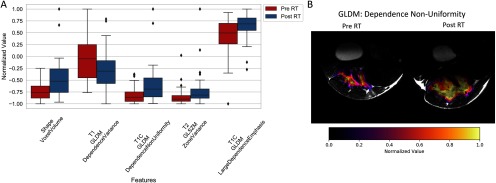
Our first radiomics analysis sought to identify tumor features that change significantly when comparing images acquired before and 1 week post RT. Figure 4A displays the most statistically significant radiomics features (both shape and texture related) between pre- and post-RT sets. The gray-level features show that after RT, tumor images often acquire a more heterogeneous texture (eg, T2 gray-level run length matrix [GLRLM]) and that the total tumor volume (ie, shape voxel volume) typically increases 1 week post RT. A spatial map of the gray-level dependence matrix (GLDM) for dependence nonuniformity is shown in Figure 4B and illustrates both the changes in gray values and shape of a tumor. In total, 76 radiomics features were found to be significantly different with RT, including 11 shape features, 23 T1-weighted texture features, 19 T1-weighted postcontrast texture features, and 23 T2-weighted texture features. This suggests that changes induced by radiation may not be limited to tumor size and shape, but also tissue properties provided in images with multiple MRI contrasts.

Figure 4.

Change in radiomic features after radiation therapy (RT). Statistically significant differences in radiomics features before and after RT as calculated from the segmented tumors (A). Spatial maps of one of the intensity-based radiomics features, the gray-level dependence non-uniformity (GLDM) (B). Differences in feature intensity are clearly visible between the 2 time points. This image also shows changes in tumor size and shape 1 week after RT.

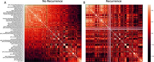
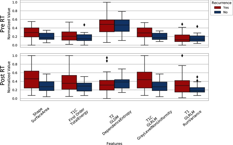
The second radiomics analysis we performed examined if radiomics features can be used to predict primary tumor recurrence in animals on study. It is important to note that all imaging was performed on the primary lesion before resection, and local recurrence would not be detectable until weeks after the second MRI date. The correlation maps of the 200 most significant radiomics features (peritumoral area, before RT) for tumors that would and would not recur are shown in Figure 5. Several regions within these maps demonstrated clear differences between features in the MRI data corresponding to animals that would eventually experience local recurrence after primary lesion excision, compared to animals in whom no recurrence was observed. A sample of radiomics features used for comparing animals in whom recurrence is observed and those who achieved successful local control is given in the plots of Figure 6. These features were calculated from the peritumoral area for both before and after RT and suggest that there may be measurable differences in radiomics features before and after RT that correlate with the potential for local recurrence (eg, T2 GLDM dependence entropy). A similar analysis was performed for the other 2 regions (tumor and tumor plus peritumoral area); however, the most visually stunning results came from the peritumoral area.

Figure 5.

Comparison of radiomic features from groups which did and did not experience primary tumor recurrence. Correlation maps of the 200 most significant of radiomics features for tumor non-recurrence (A) and recurrence (B). These data were calculated from the peritumoral area in pre-RT images. The 2 correlation maps show clear differences between features based on tumors which will and will not recur.

Figure 6.

A comparison of some of the most relevant radiomic features for predicting tumor recurrence as determined by minimum-redundancy-maximum-relevance (mRMR). Features are shown for data collected pre-RT and one-week post-RT. These features were calculated from the peritumoral area.

The features found most relevant for differentiating tumors that would eventually recur and tumors that were locally controlled came from all MR contrasts. Of the 10 radiomics features used for this purpose, 7 came gray-level features. The remaining 3 features were derived from the shape of the tumor segmentation.

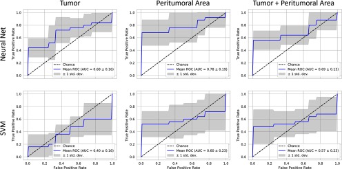
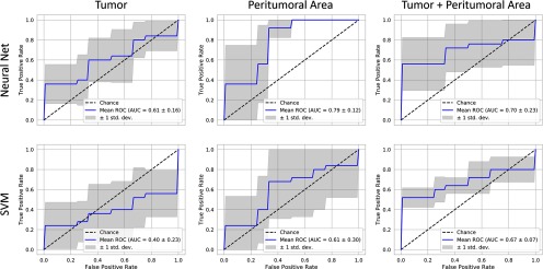
The prediction model performance is illustrated in Figures 7 (pre-RT data) and 8 (post-RT data) using plots of ROC curves for NN and SVM classifiers. The best predictive power is found from features in the peritumoral area identified using an NN and based on post-RT data (AUC: 0.79, Figure 8). These were followed closely by the performance of a NN classifier trained on the same area in the pre-RT data (AUC: 0.78). In all cases, the NN classifier outperformed the SVM.

Figure 7.

Recurrence classification from features calculated from pre-RT images receiver operating curve (ROC) curves for prediction accuracy using neural networks and support vector machines (SVMs) for 3 regions examined. The best predictive power is found from features in the peritumoral area (neural network [NN] AUC: 0.78), followed by the tumor and tumor combined with the peritumoral area (NN AUC: 0.68 vs 0.96). The NN outperforms the SVM for all regions.

Figure 8.

Recurrence classification from features calculated from post-RT images for 3 image regions. Here the best predictive power is found in the peritumoral area (NN AUC: 0.79), which is the strongest performing predictor overall. The peritumoral area shows the next strongest performance (NN AUC: 0.70 and SVM AUC: 0.67).

Discussion and Conclusions

Our results show that CNN-based segmentations with supervised learning using either T2-weighted or multicontrast MRI images are viable methods for automatic tumor volumetric measurements. Our segmentation performance (Table 2) was better in the configuration using skip connections (ie, a U-net configuration) similar to what has been reported in other studies (28). The best overall segmentation performance was achieved using a cross entropy loss, with Dice scores of 0.861 for T2-weighted images versus 0.863 for multicontrast data. When trained in K-fold cross validation, the performance drops slightly from the initial training (Table 3, mean Dice: 0.8422). This may be attributed to variation in test sets between trainings.

Automated tumor segmentation of the images before and after RT showed that tumor volumes increase in the week between the 2 imaging time points. Because a single dose of RT alone is unlikely to inhibit growth of a palpable primary lesion, these trends were expected. Gray-level intensity radiomics features indicated that tumor images acquire a more heterogeneous texture 1 week post RT. Although the administered RT was not expected to inhibit tumor growth, high-dose exposure is likely to damage tumors, causing tissue-level changes such as inflammation, edema, and necrosis. These changes alter tumor signal patterns in each of the MR contrasts, contributing to heterogeneity of the tumor radiomics features that differentiate the pre- and post-RT MRI data. This suggests that radiomics with multicontrast MRI may be useful in detecting and monitoring the effects of high-dose radiation in solid tumors.

In addition, our data suggest that radiomics features could aid in determining the likelihood of primary tumor recurrence. In our study, pre-RT data that include tumor and surrounding tissues were the most effective at identifying individuals likely to recur locally (Figure 7). Recently, peritumoral radiomics was also used to predict distant metastases in locally advanced non–small cell lung cancer (14). Although T2-weighted data alone are sufficient for tumor volume segmentation, only lagging slightly behind multimodal segmentation in performance, there are advantages in using multicontrast MRI data in radiomics analysis. This is particularly true when considering that both T1-weighted and T2-weighted scans are frequently included as standard protocols in clinical cancer imaging. In our study, the most relevant features for assessing changes over time with RT, as well as the prediction of local recurrence, were identified when including multiple MRI contrasts (Figures 4-7).

One limitation of this study is its dependence on successful and complete surgical resection of the primary tumor. A major advantage of the described mouse model is that the tumors grow and spread much like human soft tissue sarcomas, with little control by the investigators aside from site of initiation. Surgical resection of the primary lesion, just as is the case in human patients, is not always complete. It is possible that some recurrences were secondary to microscopic positive margins or regional nodal disease. Thus, surgical margins remain an important consideration when discussing local recurrence of the primary lesion. Although encouraged by our radiomics findings, we acknowledge that there are additional factors potentially confounding that cannot be evaluated by MRI data alone.

In future work, we aim to improve our prediction models by adding other biomarkers related to immune response, and we will also attempt to predict distant metastases to the lungs. More importantly, our imaging analysis pipeline will also be applied in studies adding immunotherapy to RT as part of our coclinical trial of sarcoma (11).

In conclusion, we have created and tested an image processing pipeline for high-throughput, reduced-bias segmentation of multiparametric tumor MRI data that serves the preclinical arm of our coclinical trial. Furthermore, we have implemented the architecture for radiomics analysis of tumor images, to better our understanding of preclinical imaging and the insights it provides when studying new therapeutic strategies for cancer.

References

- 1.Cormier JN, Pollock RE. Soft tissue sarcomas. CA Cancer J Clin. 2004;54:94–109. [DOI] [PubMed] [Google Scholar]
- 2.Zhang W, Li R, Deng H, Wang L, Lin W, Ji S, Shen D. Deep convolutional neural networks for multi-modality isointense infant brain image segmentation. Neuroimage. 2015;108:214–224. [DOI] [PMC free article] [PubMed] [Google Scholar]
- 3.Havaei M, Davy A, Warde-Farley D, Biard A, Courville A, Bengio Y, Pal C, Jodoin P-M, Larochelle H. Brain tumor segmentation with deep neural networks. Med Image Anal. 2017;35:18–31. [DOI] [PubMed] [Google Scholar]
- 4.Chen H, Dou Q, Yu L, Qin J, Heng PA. VoxResNet: deep voxelwise residual networks for brain segmentation from 3D MR images. Neuroimage. 2018;170:446–455. [DOI] [PubMed] [Google Scholar]
- 5.Kamnitsas K, Ledig C, Newcombe VFJ, Simpson JP, Kane AD, Menon DK, Rueckert D, Glocker B. Efficient multi-scale 3D CNN with fully connected CRF for accurate brain lesion segmentation. Med Image Anal. 2017;36:61–78. [DOI] [PubMed] [Google Scholar]
- 6.Christ PF, Ettlinger F, Grün F, Elshaera MEA, Lipkova J, Schlecht S, Ahmaddy F, Tatavarty S, Bickel M. et al. Bilic Pet al. Rempfler Met al. Hofmann Fet al. Anastasi MDet al. Ahmadi SAet al. Kaissis Get al. Holch Jet al. Sommer Wet al. Braren Ret al. Heinemann Vet al. Menze Bet al. Automatic liver and tumor segmentation of CT and MRI volumes using cascaded fully convolutional neural networks. arXiv:170205970 [cs] [Internet] 2017. Feb 20 [cited 2018 Jul 27]; Available from: http://arxiv.org/abs/1702.05970
- 7.Zhou T, Ruan S, Canu S. A review: deep learning for medical image segmentation using multi-modality fusion. Array. 2019;3–4:100004. [Google Scholar]
- 8.Gardin I, Grégoire V, Gibon D, Kirisli H, Pasquier D, Thariat J, Vera P. Radiomics: principles and radiotherapy applications. Crit Rev in Oncol/Hematol. 2019;138:44–50. [DOI] [PubMed] [Google Scholar]
- 9.Guo Z, Li X, Huang H, Guo N, Li Q. Deep learning-based image segmentation on multimodal medical imaging. IEEE Trans Radiat Plasma Med Sci. 2019;3:162–169. [DOI] [PMC free article] [PubMed] [Google Scholar]
- 10.Larue R, Defraene G, De Ruysscher D, Lambin P, van Elmpt W. Quantitative radiomics studies for tissue characterization: a review of technology and methodological procedures. Br J Radiol. 2017;90:20160665. [DOI] [PMC free article] [PubMed] [Google Scholar]
- 11.Blocker SJ, Mowery YM, Holbrook MD, Qi Y, Kirsch DG, Johnson GA, Badea CT. Bridging the translational gap: implementation of multimodal small animal imaging strategies for tumor burden assessment in a co-clinical trial. PloS One. 2019;14:e0207555 [DOI] [PMC free article] [PubMed] [Google Scholar]
- 12.Crowe EM, Alderson W, Rossiter J, Kent C. Expertise affects inter-observer agreement at peripheral locations within a brain tumor. Front Psychol. 2017;8:1628. [DOI] [PMC free article] [PubMed] [Google Scholar]
- 13.Zhang LL, Huang MY, Li Y, Liang JH, Gao TS, Deng B, Yao JJ, Lin L, Chen FP, Huang XD, Kou J, Li CF, Xie CM, Lu Y, Sun Y. Pretreatment MRI radiomics analysis allows for reliable prediction of local recurrence in non-metastatic T4 nasopharyngeal carcinoma. EBioMedicine. 2019;42:270–280. [DOI] [PMC free article] [PubMed] [Google Scholar]
- 14.Spraker MB, Wootton LS, Hippe DS, Ball KC, Peeken JC, Macomber MW, Chapman TR, Hoff MN, Kim EY, Pollack SM, Combs SE, Nyflot MJ. MRI radiomic features are independently associated with overall survival in soft tissue sarcoma. Adv Radiat Oncol [Internet]. 2019;4:413–421 [DOI] [PMC free article] [PubMed] [Google Scholar]
- 15.Lee CL, Mowery YM, Daniel AR, Zhang D, Sibley AB, Delaney JR, Wisdom AJ. et al. Qin Xet al. Wang Xet al. Caraballo Iet al. Gresham Jet al. Luo Let al. Van Mater Det al. Owzar Ket al. Kirsch DGet al. Mutational landscape in genetically engineered, carcinogen-induced, and radiation-induced mouse sarcoma. JCI Insight. 2019;4 pii: 128698. [DOI] [PMC free article] [PubMed] [Google Scholar]
- 16.Tustison N, Gee J. N4ITK: Nick’s N3 ITK implementation for MRI bias field correction. Insight J. 2009;9. [Google Scholar]
- 17.Vezhnevets V, Konouchine V. GrowCut: Interactive multi-label ND image segmentation by cellular automata In: proc of Graphicon. Citeseer; 2005. p. 150–156. [Google Scholar]
- 18.Ronneberger O, Fischer P, Brox T. U-Net: convolutional networks for biomedical image segmentation. arXiv:150504597 [cs] [Internet]. 2015 May 18; Available from: http://arxiv.org/abs/1505.04597.
- 19.Abadi M, Agarwal A, Barham P, Brevdo E, Chen Z, Citro C, Greg S Corrado, Davis A, Dean J, Devin M, Ghemawat S, Goodfellow I, Harp A, Irving G, Isard M, Jia Y, Jozefowicz R, Kaiser L, Kudlur M, Levenberg J, Mané D, Monga R, Moore S, Murray D, Olah C, Schuster M, Shlens J, Steiner B, Sutskever I, Talwar K, Tucker P, Vanhoucke V, Vasudevan V, Viégas F, Vinyals O, Warden P, Wattenberg M, Wicke M, Yu Y, Zheng X. TensorFlow: Large-Scale Machine Learning on Heterogeneous Systems. 2015. Available from: https://www.tensorflow.org/
- 20.Hinton GE, Srivastava N, Krizhevsky A, Sutskever I, Salakhutdinov RR. Improving neural networks by preventing co-adaptation of feature detectors. arXiv:12070580 [cs] [Internet]. 2012 Jul 3 [cited 2018 Jul 17]; Available from: http://arxiv.org/abs/1207.0580.
- 21.Park S, Kwak N. Analysis on the Dropout Effect in Convolutional Neural Networks In: Computer Vision – ACCV 2016 [Internet]. Springer, Cham; 2016. [cited 2018 Jul 17] p. 189–204. (Lecture Notes in Computer Science). Available from: https://link.springer.com/chapter/10.1007/978-3-319-54184-6_12. [Google Scholar]
- 22.Janson S, Vegelius J. Measures of ecological association. Oecologia. 1981;49:371–376. 1981;49: 371– [DOI] [PubMed] [Google Scholar]
- 23.Rubinstein RY, Kroese DP. The cross-entropy method: a unified approach to combinatorial optimization, Monte-Carlo simulation and machine learning. Springer Science & Business Media; 2013:316 [Google Scholar]
- 24.van der Walt S, Schönberger JL, Nunez-Iglesias J, Boulogne F, Warner JD, Yager N, Gouillart E, Yu T; scikit-image contributors. scikit-image: image processing in Python. PeerJ. 2014;2:e453. [DOI] [PMC free article] [PubMed] [Google Scholar]
- 25.Collewet G, Strzelecki M, Mariette F. Influence of MRI acquisition protocols and image intensity normalization methods on texture classification. Magn Reson Imaging. 2004;22:81–91. [DOI] [PubMed] [Google Scholar]
- 26.van Griethuysen JJM, Fedorov A, Parmar C, Hosny A, Aucoin N, Narayan V, Beets-Tan RGH. et al. Fillion-Robin JCet al. Pieper Set al. Aerts HJWL. Computational radiomics system to decode the radiographic phenotype. Cancer Res. 2017;77: e104–7. [DOI] [PMC free article] [PubMed] [Google Scholar]
- 27.Peng H, Long F, Ding C. Feature selection based on mutual information: criteria of max-dependency, max-relevance, and min-redundancy. IEEE Trans Pattern Anal Mach Intell. 2005:1226–1238. [DOI] [PubMed] [Google Scholar]
- 28.Kayalibay B, Jensen G, van der Smagt P. CNN-based segmentation of medical imaging data. arXiv:170103056 [cs] [Internet]. 2017. [cited 2018 Jul 27]; Available from: http://arxiv.org/abs/1701.03056. Here the best predictive power is found in the peritumoral area (NN AUC: 0.79), which is the strongest performing predictor overall. The peritumoral area shows the next strongest performance (NN AUC: 0.70 and SVM AUC: 0.67).